Statistical inference for exponential functionals of Lévy processes

Abstract

In this paper, we consider the exponential functional $A_{\infty}=\int_{0}^{\infty}e^{-\xi_{s}}ds$ of a Lévy process $\xi_{s}$ and aim to estimate the characteristics of $\xi_{s}$ from the distribution of $A_{\infty}$. We present a new approach, which allows to statistically infer on the Lévy triplet of $\xi_{t}$, and study the theoretical properties of the proposed estimators. The suggested algorithms are illustrated with numerical simulations.

T1This research was partially supported by the Deutsche Forschungsgemeinschaft through the SFB 823 “Statistical modelling of nonlinear dynamic processes” and by Laboratory for Structural Methods of Data Analysis in Predictive Modeling, MIPT, RF government grant, ag. 11.G34.31.0073.

1 Introduction

For a Lévy process $\xi=\left(\xi_{t}\right)_{t\geq 0}$, the exponential functional of $\xi$ is defined by

$$A_{t}=\int_{0}^{t}e^{-\xi_{s}}\;ds,$$

where $t\in(0,\infty)$. The main object of this research is the terminal value

$$A_{\infty}:=\lim_{t\to\infty}A_{t}=\int_{0}^{\infty}e^{-\xi_{s}}\;ds,$$ (1)

which often (and everywhere in this paper) is called also an exponential functional of $\xi$. The integral $A_{\infty}$ naturally arises in a wide variety of financial applications as an invariant distribution of the process

$$V_{t}=e^{-\xi_{t}}\left(V_{0}+\int_{0}^{t}e^{\xi_{s-}}ds\right),$$ (2)

see Carmona, Petit, Yor [10]. For instance, the process (2) determines the volatility process in the COGARCH (COntinious Generalized AutoRegressive Conditionally Heteroscedastic) model introduced by Klüppelberg et al. [17]. Note that $V_{t}$ is in fact a partial case of the generalized Ornstein-Uhlenbeck (GOU) process. A comprehensive study of the GOU model is given in the dissertation by Behme [2].

$A_{\infty}$ appears in finance also in other contexts, for instance, in pricing of Asian options, see the monograph by Yor [30] and the references given by Carmona, Petit, Yor [10]. As for other fields of applications, $A_{\infty}$ plays a crucial role in studying the carousel systems (see Litvak and Adan [21], Litvak and Zwet [22]), self-similar fragmentations (see Bertoin and Yor [8]), and information transmission problems (especially TCP/IP protocol, see Guillemin, Robert and Zwart [15]). For the detailed discussion of the physical interpretations, we refer to Comtet, Monthus and Yor [11] and the dissertation by Monthus [24].

Denote the Lévy triplet of the process $\xi_{t}$ by $(c,\sigma,\nu)$, i.e.,

$$\xi_{t}=ct+\sigma W_{t}+\mathcal{T}_{t},$$ (3)

where $\mathcal{T}_{t}$ is a pure jump process with Lévy measure $\nu$. The finiteness condition stands that the integral $A_{\infty}$ is finite if and only if $\xi_{t}\to+\infty$ as $t\to+\infty$, see Maulik and Zwart [23] for the proof and Erickson and Maller [14] for some extensions of this result. Therefore, the integral $A_{\infty}$ is finite if the process $\xi_{t}$ is any non-degenerated subordinator, i.e., any non-decreasing Lévy process, or, equivalently, any non-negative Lévy process. Nevertheless, the finiteness condition is fulfilled for other processes also, e.g., for $\xi_{t}=-N_{t}+2\lambda t$, where $N_{t}$ is a Poisson process with intensity $\lambda$.

In this paper, we mainly focus on the case when $\xi$ is a subordinator with finite Lévy measure. In terms of the Lévy triplet, this means that $c>0$, $\sigma=0$, $\nu(I\!\!R_{-})=0$ and moreover $a:=\nu(I\!\!R_{+})<\infty$. Suppose that the process (2) is observed in the time points $0=t_{0}<t_{1}<...<t_{n}$. Taking into account that the process $V_{t}$ is a Markov process, and assuming that $V_{0}$ has an invariant distribution determined by $A_{\infty}$, we conclude that $V_{t_{0}},...,V_{t_{n}}$ have also the distribution of $A_{\infty}$. The main goal of this research is to statistically infer on the Lévy triplet of $\xi$ from the observations $V_{t_{0}},...,V_{t_{n}}$. More precisely, we will pursue the following two aims: (1) to estimate the drift term $c$ and the parameter $a$; (2) to estimate the Lévy measure $\nu$.

To the best of our knowledge, the statistical inference for exponential functionals of Lévy processes has not been previously considered in the literature. However, some distributional properties of the exponential functionals are well-known, e.g., the integro - differential equation by Carmona, Petit, Yor [9]. For the overview of theoretical results, we refer to the survey by Bertoin and Yor [8]. One distribution property, the recursive formula for the moments of $A_{\infty}$, gives rise to the approach presented in our paper. This result stands that

$${\mathbb{E}}\left[A_{\infty}^{s-1}\right]=\frac{\psi(s)}{s}\;{\mathbb{E}}\left[A_{\infty}^{s}\right],$$ (4)

where $\psi(s)$ is a Laplace exponent of the process $\xi$, i.e., $\psi(s):=-\log{\mathbb{E}}\left[e^{-s\xi_{1}}\right],$ and complex $s$ is taken from the area

$$\Upsilon:=\Bigl{\{}s\in{\mathbb{C}}:\;0<\operatorname{Re}(s)<\theta\Bigr{\}}\quad\mbox{with}\quad\theta:=\sup\left\{z\geq 0:{\mathbb{E}}[e^{-z\xi_{1}}]\leq 1\right\}.$$ (5)

The recursive formula (4) firstly appear for real $s$ in the paper by Maulik and Zwart [23]. The complete proof for complex $s$ was given recently by Kuznetsov, Pardo and Savov [20]. If $\xi_{t}$ is a subordinator, what is the case under our setup, the parameter $\theta$ is equal to infinity.

The idea of the procedure for solving the first task (estimation of $a$ and $c$) is to infer on the parameters of the process $\xi$ from its Laplace exponent. First, making use of (4), we estimate the Laplace exponent $\psi(s)$ at the points $s=u+\mathrm{i}v\in\Upsilon$, where $u$ is fixed and $v$ varies on the equidistant grid between $\varepsilon V_{n}$ and $V_{n}$ (with $\varepsilon>0$ and $V_{n}\to\infty$ as $n\to\infty$) Afterwards, we take into account that

$$\psi(u+\mathrm{i}v) = a+c\left(u+\mathrm{i}v\right)-\mathcal{F}_{\bar{\nu}}(-v),\qquad u,v\in I\!\!R,$$ (6)

where $\bar{\nu}(dx):=e^{-ux}\nu(dx)$, and $\mathcal{F}_{\bar{\nu}}(v)$ stands for the Fourier transform of the measure $\bar{\nu}$, i.e., $\mathcal{F}_{\bar{\nu}}(v):=\int_{I\!\!R_{+}}e^{\mathrm{i}vx}\bar{\nu}(dx).$ It is worth mentioning that $\mathcal{F}_{\bar{\nu}}(v)\to 0$ as $v\to\infty$, and therefore taking the real and imaginary parts of the left and right hand sides of (6), we are able to consequently estimate the parameters $c$ and $a$.

With no doubt, the second aim (complete recovering of the Lévy measure) is the most challenging task. Since the estimates of the parameters $c$ and $a$ are already obtained, we can estimate by (6) the Fourier transform $\mathcal{F}_{\bar{\nu}}(v)$ for $v$ taken from the equidistant grid $[-V_{n},V_{n}]$. The last step of this procedure, estimation of the Lévy measure $\nu$, is based on the inverse Fourier transform formula, and reveals the main reason for using the complex numbers in our approach. In fact, one can estimate the function $\psi(\cdot)$ in real points and then estimate the Laplace transform of the measure $\nu$ by the regression arguments. In this case, estimation of $\nu$ demands the inverse Laplace transform, which is given by Bromwich integral and therefore is in fact much more involved in comparison with the inverse Fourier transform.

The paper is organized as follows. In the next section, we introduce the assumptions on this model and give some examples. We formulate the algorithms for estimation the Laplace exponent $\psi(s)$ (Section 3.1), the parameters $a$ and $c$ (Section 3.2), and the Lévy measure $\nu$ (Section 3.3). Next, we provide some numerical examples in Section 4 and analyze the convergence rates of the proposed algorithms in Section 5. Appendix contains some related results and additional proofs.

2 Assumptions on the model

2.1 Subordinators

In this article, we restrict our attention to the case when the following set of assumptions is fulfilled:

(A1)

$$\left\{\begin{aligned} c\geq 0,&\qquad\sigma=0,\\ \nu(I\!\!R_{-})=0,&\qquad a:=\nu(I\!\!R_{+})<\infty.\\ \end{aligned}\right.$$

This set in particularly yields that the process $\xi$ has finite variation, i.e.,

$$\int_{I\!\!R_{+}}\left(x\wedge 1\right)\nu(dx)<\infty,$$ (7)

and therefore $\xi$ is a non-decreasing Lévy processes, i.e., a subordinator. The detailed discussion of the subordination theory as well as various examples of such processes (Gamma, Poisson, tempered stable, inverse Gaussian, Meixner processes, etc.), are given in [1], [7], [12], [26], [27].

Note that in the case of subordinators, the truncation function in the Lévy-Khinchine formula can be omitted, and therefore the characteristic exponent of $\xi$ is equal to

$$\psi_{e}(s)=\log{\mathbb{E}}\left[e^{\mathrm{i}s\xi_{1}}\right]=\mathrm{i}cs+\int_{0}^{\infty}\left(e^{\mathrm{i}sx}-1\right)\nu(dx).$$ (8)

Later on, we use a Laplace exponent of $\xi$, which is defined by

$$\psi(s):=-\log{\mathbb{E}}\left[e^{-s\xi_{1}}\right]=-\psi_{e}\left(\mathrm{i}s\right),$$

and under the assumption (A1) is equal to

$$\psi(s) = cs+\int_{0}^{\infty}\left(1-e^{-sx}\right)\nu(dx)$$ (9)

$$= cs+s\int_{0}^{\infty}e^{-sx}\nu(x,+\infty)dx.$$ (10)

Some examples can be found in Section 4. In the sequel, we use the fact that the function $\psi(\cdot)$ is bounded from above on the set $\Upsilon$ by

$$|\psi(s)| \leq c|s|+\int_{0}^{\infty}\left(1+e^{-\operatorname{Re}(s)x}\right)\nu(dx)\leq c\sqrt{\theta^{2}+\operatorname{Im}^{2}(s)}+2a,$$

and hence the asymptotic behavior of the function $\psi(s)$ is given by

$$\left|\psi(s)\right|=O\Bigl{(}\operatorname{Im}(s)\Bigr{)},\qquad\operatorname{Im}(s)\to+\infty.$$ (11)

2.2 Further assumptions on $\nu$

First, we assume the following asymptotic behavior of the Mellin transform of the integral $A_{\infty}$:

(A2)

$\hskip 85.35826pt\left|{\mathbb{E}}\left[A_{\infty}^{u^{\circ}+\mathrm{i}v}\right]\right|\asymp\exp\{-\gamma|v|\},\qquad\mbox{as }\;|v|\to\infty$

with some $\gamma>0$ and $u^{\circ}>0$.

Second, we introduce an assumption on the measure $\bar{\nu}(dx):=e^{-u^{\circ}x}\nu(dx)$ :

(A3)

$\hskip 113.81102pt\left\|\bar{\nu}^{(r)}\right\|_{L^{\infty}(I\!\!R)}\leq C$

for some positive $r$ and $C$.

It is worth noting that there is an (indirect) relation between the assumptions (A2) and (A3). In fact, joint consideration of (4) and (6) yields that

$$\mathcal{F}_{\bar{\nu}}(-v) = a+c\left(u^{\circ}+\mathrm{i}v\right)-(u^{\circ}+\mathrm{i}v)\frac{m(u^{\circ}+\mathrm{i}v)}{m((u^{\circ}+1)+\mathrm{i}v)},\qquad u,v\in I\!\!R,$$

where $m(s):={\mathbb{E}}\left[A_{\infty}^{s-1}\right]$ is the Mellin transform.

Example 1. For instance, the set of assumptions (A1) - (A3) fulfills for the class of Lévy processes with $c=0$ and Lévy density in the form

$$\nu(x)=I_{x>0}\sum_{j=1}^{M}\sum_{k=1}^{{m_{j}}}\alpha_{jk}x^{k-1}e^{-\rho_{j}x}$$

with $M,m_{j}\in{\mathbb{N}}$, $\rho_{j}>0$, $\alpha_{jk}>0$. In fact, assumption (A1) and (A3) obviously hold; assumption (A2) is checked in [19] for any positive $u^{\circ}$ (p. 658, the proof of Theorem 1).

Example 2. Next, we provide an example of the Lévy process which doesn’t possess the property (A2). Consider a subordinator $\mathcal{T}$ with drift $c>0$ and the Lévy density

$$\nu(x)=ab\exp\{-bx\}\>I\{x>0\},\quad a,b>0,$$

which we describe in details in Section 4. The exponential functional of this process has a density

$$k(x)=C_{1}x^{b}(1-cx)^{(a/c)-1}\>I\{0<x<1/c\}$$

with some $C_{1}>0$, see [9]. In other words, the exponential functional has a distribution $B(\alpha+1,\beta+1)/c$, where $B$ stands for Beta distribution with parameters $\alpha=b$ and $\beta=a/c-1$. The Mellin transform of the function $k(x)$ in the half -plane $\operatorname{Re}(s)>-\alpha$ is given by

$$m(s)=C_{2}(\alpha,\beta)\>c^{s}\>\frac{\Gamma(\alpha+s)}{\Gamma(\alpha+\beta+1+s)},$$

where $C_{2}(\alpha,\beta)>0$, see Table 1 from [13]. Taking into account the following asymptotical behavior of the Gamma function

$$\left|\Gamma(u+\mathrm{i}v)\right|=\exp\left\{-\frac{\pi}{2}v+\left(u-\frac{1}{2}\right)\ln v+O(1)\right\},\qquad v\to\infty,$$

see (9) from [19], we conclude that the exponential functional of the process $\mathcal{T}$ has a polynomial decay of the Mellin transform. More precisely, $|m(s)|\asymp C_{3}v^{-a/c-1}$ with some $C_{3}>0$.

3 Estimation of the Lévy triplet

In the sequel, suppose that the process (2) is observed at the time points $0=t_{0}<t_{1}<...<t_{n}$. Assuming that $V_{0}$ has a stationary invariant distribution, we get that the values $A_{\infty,k}:=V_{t_{k}},\;k=1..n$ have the distribution of the integral $A_{\infty}$.

3.1 Estimation of the Laplace exponent

The first step of the estimation procedure is to construct the estimate of the function $\psi(s)$ in the complex points $s=u+\mathrm{i}v$, where $u$ is fixed and $v$ varies. The reason for such choice of $s$ is clear from the further steps of the algorithm.

The estimator of $\psi(s)$ is based on a recursive formula for the $s-$th (complex) moment of $A_{\infty}$:

$${\mathbb{E}}\left[A_{\infty}^{s-1}\right]=\frac{\psi(s)}{s}\;{\mathbb{E}}\left[A_{\infty}^{s}\right],$$ (12)

In [9], this formula is proved for real positive $s$ such that $\psi(s)>0$ and ${\mathbb{E}}\left[A_{\infty}^{s}\right]<\infty$. The case of infinite mathematical expectations is carefully discussed in [23].

The case of complex $s$ is considered in [20], where one can find also some generalizations of the formula (12) for integrals with respect to the Brownian motion with drift. In particular, applying Theorem 2 from [20], we get that (12) holds for any $s\in\Upsilon$. In the situation when $\xi_{t}$ is a subordinator, the set $\Upsilon$ coincides with the positive half-plane (equivalently, the parameter $\theta$ is equal to infinity), because it follows from (10) that

$${\mathbb{E}}\left[e^{-s\xi_{1}}\right]=-\psi(-s)=-cs-s\int_{I\!\!R_{+}}e^{sx}\nu(x,+\infty)dx<0,\quad s>0.$$

Motivated by (12), we now present the the first two steps in the estimation procedure. Let the values $\alpha_{1},...,\alpha_{M}$ compose the equidistant grid with the step $\Delta>0$ on the set $[\varepsilon,1]$, where $\varepsilon>0$ and the sequence $V_{n}$ tends to infinity. First, we estimate $A_{\infty}^{s}$ for $s=u+\mathrm{i}\alpha_{m}V_{n},\;m=1..M$ and $s=(u-1)+\mathrm{i}v_{m},\;m=1..M$ where $u:=u^{\circ}\in\left(-1,\theta\right)$ satisfies the assumptions (A2) and (A3). Theoretical studies (see Section 5) show that the optimal choice is $V_{n}=\kappa\log(n)$ with $\kappa<1/(2\gamma)$, provided that the Assumptions (A1)-(A3) hold. The estimator of $A_{\infty}^{s}$ is defined by

$$\widehat{\mathbb{E}}_{n}\left[A_{\infty}^{s}\right]=\frac{1}{n}\sum_{k=1}^{n}A_{\infty,k}^{s}.$$ (13)

Next, we define an estimate of $\psi(\cdot)$ at the points $\left(u+\mathrm{i}\alpha_{m}V_{n}\right)$ by

$$\hat{\psi}_{n}(u+\mathrm{i}\alpha_{m}V_{n})=\left(u+\mathrm{i}\alpha_{m}V_{n}\right)\;\frac{\widehat{\mathbb{E}}_{n}\left[A_{\infty}^{(u-1)+\mathrm{i}\alpha_{m}V_{n}}\right]}{\widehat{\mathbb{E}}_{n}\left[A_{\infty}^{u+\mathrm{i}\alpha_{m}V_{n}}\right]},\qquad m=1..M.$$ (14)

The performance of this estimator is later shown in Section 4, see in particularly Figures 1 and 3. The quality of $\hat{\psi}_{n}(\cdot)$ is theoretically studied in Theorem 5.1, which stands that under the assumptions (A1) and (A2) and the following condition on $V_{n}$

$$\Lambda_{n}:=V_{n}\exp\left\{cV_{n}\right\}\sqrt{\log V_{n}}=o\left(\sqrt{\frac{n}{\log(n)}}\right),\;n\to\infty,$$

it holds for $n$ large enough

$${\mathbb{P}}\Biggl{\{}\sup_{v\in[\varepsilon V_{n},V_{n}]}\left|\hat{\psi}_{n}(u+\mathrm{i}v)-\psi(u+\mathrm{i}v)\right|\leq\beta\>\Lambda_{n}\sqrt{\frac{\log(n)}{n}}\Biggr{\}}>1-\alpha n^{-1-\delta},$$ (15)

with some positive $\alpha$, $\beta$ and $\delta$.

3.2 Estimation of $a$ and $c$

In Section 2.1, we present the representation (9) for the Laplace exponent of the process $\xi$. Substituting now the complex argument $z=u+\mathrm{i}v$, we get

$$\psi(u+\mathrm{i}v) = c\left(u+\mathrm{i}v\right)-\int_{I\!\!R_{+}}e^{-\mathrm{i}vx}\bar{\nu}(dx)+\int_{I\!\!R_{+}}\nu(dx)$$ (16)

$$= c\left(u+\mathrm{i}v\right)-\mathcal{F}_{\bar{\nu}}(-v)+a,\qquad u,v\in I\!\!R,$$

where $a:=\int_{I\!\!R_{+}}\nu(dx)$ and $\bar{\nu}(dx):=e^{-ux}\nu(dx)$. The general idea of the procedure described below is to estimate the Laplace exponent $\psi(\cdot)$ at the points $s=u+\mathrm{i}v$, where $u$ is fixed at $v$ varies (see Section 3.1), and afterwards to use (16) for consequent estimation of the parameters.

Taking imaginary and real of both hand sides in (16), we get

$$\operatorname{Im}\psi(u+\mathrm{i}v) = cv-\operatorname{Im}\mathcal{F}_{\bar{\nu}}(-v),$$ (17)

$$\operatorname{Re}\psi(u+\mathrm{i}v) = cu-\operatorname{Re}\mathcal{F}_{\bar{\nu}}(-v)+a.$$ (18)

By Riemann - Lebesque lemma, $\mathcal{F}_{\bar{\nu}}(-v)\to 0$ as $v\to+\infty$, see, e.g., [16]; note that the rates of this convergence are assumed in (A3). Therefore, looking at (17), we conclude that $\operatorname{Im}\psi(u+\mathrm{i}v)$ is a (asymptotically) linear in $v$ function, and the parameter $c$ can be interpreted a slope parameter. Next, from (18), it follows that $\operatorname{Re}\psi(u+\mathrm{i}v)$ tends to $(cu+a)$ as $v\to+\infty$. These observations lead to the following optimization problems

$$\tilde{c}_{n} := \operatornamewithlimits{arg\,min}_{c}\int_{I\!\!R_{+}}w_{n}(v)\Bigl{(}\operatorname{Im}\hat{\psi}_{n}(u+\mathrm{i}v)-cv\Bigr{)}^{2}dv$$ (19)

$$\tilde{a}_{n} := \operatornamewithlimits{arg\,min}_{a}\int_{I\!\!R_{+}}w_{n}(v)\Bigl{(}\operatorname{Re}\hat{\psi}_{n}(u+\mathrm{i}v)-\tilde{c}_{n}u-a\Bigr{)}^{2}dv,$$ (20)

where the weighting function is chosen in the form $w_{n}(v)=w(v/V_{n})/V_{n}$ with an integrable non-negative function $w(\cdot)$ supported on $[\varepsilon,1]$. Under this choice of $V_{n}$, we can rewrite (19) as follows:

$$\tilde{c}_{n} := \operatornamewithlimits{arg\,min}_{c}\int_{\varepsilon}^{1}w(\alpha)\Bigl{(}\operatorname{Im}\hat{\psi}_{n}(u+\mathrm{i}\alpha V_{n})-c\alpha V_{n}\Bigr{)}^{2}dv$$

$$\tilde{a}_{n} := \operatornamewithlimits{arg\,min}_{a}\int_{\varepsilon}^{1}w(\alpha)\Bigl{(}\operatorname{Re}\hat{\psi}_{n}(u+\mathrm{i}\alpha V_{n})-\tilde{c}_{n}u-a\Bigr{)}^{2}dv,$$

In practice, we first get the estimates of the Laplace exponent at the points $s=u+\mathrm{i}\alpha_{m}V_{n}$ (see above) and define an estimate of the parameter $c$ by

$$\hat{c}_{n} := \operatornamewithlimits{arg\,min}_{c}\sum_{m=1}^{M}w(\alpha_{m})\Bigl{(}\operatorname{Im}\hat{\psi}_{n}(u+\mathrm{i}\alpha_{m}V_{n})-c\alpha_{m}V_{n}\Bigr{)}^{2}$$ (21)

$$= \frac{\sum_{m=1}^{M}w(\alpha_{m})\alpha_{m}\>\operatorname{Im}\hat{\psi}_{n}(u+\mathrm{i}\alpha_{m}V_{n})}{V_{n}\>\cdot\>\sum_{m=1}^{M}w(\alpha_{m})\alpha_{m}^{2}}.$$ (22)

Afterwards, we estimate the parameter $a$ by

$$\hat{a}_{n} := \operatornamewithlimits{arg\,min}_{a}\sum_{m=1}^{M}w(\alpha_{m})\Bigl{(}\operatorname{Re}\hat{\psi}_{n}(u+\mathrm{i}\alpha_{m}V_{n})-\hat{c}_{n}u-a\Bigr{)}^{2}$$ (23)

$$= \frac{\sum_{m=1}^{M}w(\alpha_{m})\operatorname{Re}\hat{\psi}_{n}(u+\mathrm{i}\alpha_{m}V_{n})}{\sum_{m=1}^{M}w(\alpha_{m})}-\hat{c}_{n}u.$$ (24)

We show empirical and theoretical properties of the estimators $\hat{a}_{n}$ and $\hat{c}_{n}$ below, see Figure 2 and Theorem 5.3. Similar to (15), we prove that under the choice $V_{n}=\kappa\log(n)$ with $\kappa<1/(2\gamma)$, it holds

$${\mathbb{P}}\Biggl{\{}\left|\tilde{c}_{n}-c\right|\leq\zeta_{1}\log^{-(r+2)}(n)\Biggr{\}} > 1-\alpha n^{-1-\delta},\qquad\mbox{and}$$

$${\mathbb{P}}\Biggl{\{}\left|\tilde{a}_{n}-a\right|\leq\zeta_{2}\log^{-(r+1)}(n)\Biggr{\}} > 1-\alpha n^{-1-\delta},$$

with $\zeta_{1},\zeta_{2}>0$, and $\alpha,\delta$ introduced above. Constants $\gamma$ and $r$ involved in this statement are comming from assumptions (A2) and (A3) resp. Moreover, we prove Theorem 5.4, which stands that this rate for $c$ is optimal one in the class $\mathscr{A}$ of the models satisfying the assumptions (A1) - (A3). More precisely, we show that

$$\varliminf_{n\to\infty}\inf_{\tilde{c}_{n}^{*}}\sup_{\mathscr{A}}{\mathbb{P}}\Biggl{\{}\left|\tilde{c}_{n}^{*}-c\right|\geq\zeta_{3}\log^{-(r+2)}(n)\Biggr{\}}>0,$$

where $\zeta_{3}<\zeta_{1}$ is some positive constant, the supremum is taken over all models from $\mathscr{A}$, and infimum - over all possible estimates of the parameter $c$.

We summarize the steps discussed above in the following algorithm.

[couleur=blue!15, logo=] Algorithm 1: Estimation of $a$ and $c$

Data: $n$ observations $A_{\infty,1},...,A_{\infty,n}$ of the integral $A_{\infty}=\int_{I\!\!R_{+}}\exp\{-\xi_{s}\}ds$,

where $\xi=\left(\xi_{t}\right)_{t\geq 0}$ is a Lévy process with unknown Lévy triplet $\left(c,0,\nu\right)$.

Take $V_{n}=\kappa\log(n)$ with $\kappa<1/(2\gamma)$, fix $\varepsilon\in(0,1)$ and $u>-1$.

Take the values $\alpha_{1},...,\alpha_{M}$ on the equidistant grid on the set $[\varepsilon,1]$ with a step $\Delta$.

Define a function $w(\cdot)\geq 0$ supported on $[\varepsilon,1]$. Denote $v_{m,n}:=\alpha_{m}V_{n}$.

1. Estimate $A_{\infty}^{s}$ for $s=u_{j}+\mathrm{i}v_{m,n},\;m=1..M,$ where $u_{1}=u$ and $u_{2}=u-1$

   $$\widehat{\mathbb{E}}_{n}\left[A_{\infty}^{u_{j}+\mathrm{i}v_{m,n}}\right]=\frac{1}{n}\sum_{k=1}^{n}A_{\infty,k}^{u_{j}+\mathrm{i}v_{m,n}},\qquad m=1..M,\quad j=1,2.$$

2. Estimate $\psi(u+\mathrm{i}v_{m,n})$ by

   $$\hat{\psi}_{n}(u+\mathrm{i}v_{m,n})=\left(u+\mathrm{i}v_{m,n}\right)\;\frac{\widehat{\mathbb{E}}_{n}\left[A_{\infty}^{\left(u-1\right)+\mathrm{i}v_{m,n}}\right]}{\widehat{\mathbb{E}}_{n}\left[A_{\infty}^{u+\mathrm{i}v_{m,n}}\right]},\qquad m=1..M.$$

3. Estimate $c$ by the solution of the optimization problem (21),

   which is explicitly given by

   $$\hat{c}_{n}:=\frac{\sum_{m=1}^{M}w(\alpha_{m})\alpha_{m}\>\operatorname{Im}\hat{\psi}_{n}(u+\mathrm{i}v_{m,n})}{V_{n}\>\cdot\>\sum_{m=1}^{M}w(\alpha_{m})\alpha_{m}^{2}}.$$

4. Estimate $a$ by the solution of the optimization problem (23),

   which is explicitly given by

   $$\hat{a}_{n}:=\frac{\sum_{m=1}^{M}w(\alpha_{m})\operatorname{Re}\hat{\psi}_{n}(u+\mathrm{i}v_{m,n})}{\sum_{m=1}^{M}w(\alpha_{m})}-\hat{c}_{n}u.$$

3.3 Recovering the Lévy measure $\nu$

As the result of the algorithm described below, we obtain the estimates $\hat{c}_{n}$ and $\hat{a}_{n}$ of the parameters $c$ and $a$. In this subsection, we present the algorithm for estimation the Lévy measure $\nu$.

First, we take points $s=u+\mathrm{i}\alpha_{m}V_{n}$, where $\alpha_{m},$  $m=1..M$, belong to the interval $[-1,1]$. The construction of the estimates $\hat{\psi}_{n}(s)$ remains the same as in Section 3.1. Next, looking at (16), we define an estimate $\mathcal{F}_{\bar{\nu}}(-v)$ for $v=\alpha_{m}V_{n},\>m=1..M$ by

$$\hat{\mathcal{F}}_{\bar{\nu}}(-v)=-\hat{\psi}_{n}(u+\mathrm{i}v)+\hat{c}_{n}(u+\mathrm{i}v)+\hat{a}_{n}.$$ (25)

The last step is to recover the measure $\nu$ from the estimator of the Fourier transform of the measure $\bar{\nu}$. Motivated by the inverse Fourier transform formula, we propose the following nonparametric estimator of the measure $\nu$:

$$\tilde{\nu}(x) = \frac{1}{2\pi}e^{ux}\int_{I\!\!R}e^{\mathrm{i}vx}\hat{\mathcal{F}}_{\bar{\nu}}(-v)\mathcal{K}(vh_{n})dv,$$ (26)

where $\mathcal{K}$ is a regularizing kernel supported on $[-1,1]$ and $h_{n}$ is a sequence of bandwidths which tends to $0$ as $n\to\infty$. The formal description of the algorithm is given below.

[couleur=blue!15, logo=] Algorithm 2: Estimation of $\nu$

Data: $n$ observations $A_{\infty,1},...,A_{\infty,n}$ of the integral $A_{\infty}=\int_{I\!\!R_{+}}\exp\{-\xi_{s}\}ds$,

where $\xi=\left(\xi_{t}\right)_{t\geq 0}$ is a Lévy process with unknown Lévy triplet $\left(c,0,\nu\right)$. The estimates $\hat{a}_{n}$ and $\hat{c}_{n}$ are described in Algorithm 1.

Take the values $\alpha_{1},...,\alpha_{M}$ on the equidistant grid on the set $[-1,1]$ with a step $\Delta$.

Denote $v_{m,n}:=\alpha_{m}V_{n}$.

Define a regularizing kernel $\mathcal{K}$ supported on $[-1,1]$, and a (large enough) number $h$.

1. The first two steps coincide with given in Algorithm 1.

2. Estimate $\mathcal{F}_{\bar{\nu}}(-v_{m,n})$ for $\bar{\nu}(dx)=e^{-ux}\nu(dx)$ by

   $$\hat{\mathcal{F}}_{\bar{\nu}}(-v_{m,n})=-\hat{\psi}_{n}(u+\mathrm{i}v_{m,n})+\hat{c}_{n}\cdot(u+\mathrm{i}v_{m,n})+\hat{a}_{n},\,m=1..M.$$

3. Estimate $\nu$ by

   $$\hat{\nu}(x) = e^{ux}\frac{\Delta}{2\pi}\sum_{m=1}^{M}e^{\mathrm{i}v_{m,n}x}\hat{\mathcal{F}}_{\bar{\nu}}(-v_{m,n})\mathcal{K}(v_{m,n}h).$$

Some theoretical and practical aspects of this algorithm are discussed in Sections 4 and 5.

Remark 3.1.

It is a worth mentioning that the estimation algorithms 1 and 2 can be applied to more general situation when the process $\mathcal{T}_{t}$ is a difference between two subordinators, i.e., $\mathcal{T}_{t}=\mathcal{T}^{+}_{t}+\mathcal{T}^{-}_{t}$, where $\mathcal{T}^{+}$ and $\mathcal{T}^{-}$ are the processes of finite variation with Lévy measures $\nu^{+}$ and $\nu^{-}$ concentrated on $I\!\!R_{+}$ and $I\!\!R_{-}$ resp. In fact, in this case, the formula (16) still holds with

$$\nu(dx)=I\!\!I\{x>0\}\nu^{+}(dx)+I\!\!I\{x<0\}\nu^{-}(dx).$$

Therefore, the consequent estimation of $c$, $a$ and the Fourier transform of the measure $e^{-ux}\nu(dx)$, as well as the estimation of $\nu$ are still possible.

Theoretical results under the assumptions (A2) and (A3) remain the same. The example from Section 2.2 can be naturally extended to

$$\nu(x)=I_{x>0}\sum_{j=1}^{M}\sum_{k=1}^{{m_{j}}}\alpha_{jk}x^{k-1}e^{-\rho_{j}x}+I_{x<0}\sum_{j=1}^{\tilde{M}}\sum_{k=1}^{{\tilde{m}_{j}}}\tilde{\alpha}_{jk}x^{k-1}e^{-\tilde{\rho}_{j}x}$$

with $M,\tilde{M},m_{j},\tilde{m}_{j}\in{\mathbb{N}}$, $\rho_{j},\tilde{\rho}_{j}>0$, $\alpha_{jk},\tilde{\alpha}{jk}>0$. Note that Assumption (A2) is already checked in Theorem 1 from [19].

4 Simulation study

Example 1. Consider the subordinator $\mathcal{T}_{t}$ with the Lévy density

$$\nu(x)=ab\exp\{-bx\}\>I\{x>0\},\quad a,b>0.$$ (27)

For this subordinator, the integral $A_{\infty}$ is finite for any $\sigma$, see [9]. The Laplace exponent of $\xi$ is given by

$$\psi(z)=z\left(c-\frac{1}{2}\sigma^{2}z+\frac{a}{b+z}\right).$$ (28)

As for the distribution properties of $A_{\infty}$, the density function of $A_{\infty}$ satisfies the following differential equation

$$-\frac{\sigma^{2}}{2}x^{2}k^{\prime\prime}(x)+\left[\left(\frac{\sigma^{2}}{2}(3-b)+c\right)x-1\right]k^{\prime}(x)\\ +\left[\left(1-b\right)\left(\frac{\sigma^{2}}{2}+c\right)-a+\frac{b}{x}\right]k(x)=0,$$ (29)

see [9]. Some typical situations are given below:

1. In the case $c=0,\>\sigma=0$ (pure jump process), this equation has a solution

   $$k_{1}(x)=Cx^{b}e^{-ax}\>I\{x>0\},$$ (30)

   and therefore $A_{\infty}\buildrel d\over{G}(b+1,a)$, where $G(\alpha,\beta)$ is a Gamma distribution with shape parameter $\alpha$ and rate $\beta$.

2. If $c>0,\>\sigma=0$ (pure jump process with drift), then

   $$k_{2}(x)=Cx^{b}(1-cx)^{(a/c)-1}\>I\{0<x<1/c\}.$$ (31)

   In this situation $A_{\infty}\buildrel d\over{B}(b+1,a/c)/c$, where $B(\alpha,\beta)$ is a Beta - distribution.

3. In the case $c\neq 0,\>\sigma\neq 0$, the equation (29) also allows for the closed form solutions. Assuming for simplicity $\sigma^{2}/2=1$, $c=-(b+1)$, we get the solution of (29) in the following form:

   $$k_{3}(x)=C\>x^{b-1/2}\exp\left\{\frac{1}{2x}\right\}I_{\mu}\left(\frac{1}{2x}\right),$$ (32)

   where we denote by $I_{\mu}$ the modified Bessel function of the first kind, $\mu=\sqrt{a+1/4}$, and the constant $c$ is later chosen to guarantee the condition $\int_{0}^{\infty}k_{3}(x)dx=1$.

For the numerical study, we assume that the data follows the model (1) where the process $\xi_{t}$ is defined by (3) with $c=1.8$, $\sigma=0$, and the subordinator $\mathcal{T}_{t}$ has a Lévy density in the form (27) with $a=0.7$, $b=0.2$. The values of the integral $A_{\infty}$ are simulated from the Beta-distribution, see (31).

On the first step, we estimate $A_{\infty}^{s}$ for $s=u+\mathrm{i}v$ with $u=29$ and $u=30$ and $v$ from the equidistant grid between $-30$ and $30$. Next, we estimate the Laplace exponent by the formula (14). One can visually compare the proposed estimator and the theoretical value $(c+a/(b+s))*s$ looking at Figure 1.

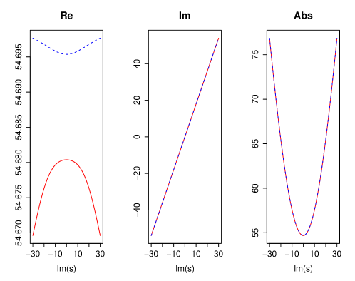
Figure 1: Plots of theoretical (blue dashed) and empirical (red solid) Laplace exponents for Example 1. Graphs present real, imaginary parts and absolute values. In spite of visual distinction in the real parts, the difference between theoretical and empirical Laplace exponents is quite small.

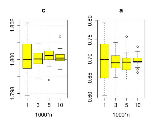
Figure 2: Boxplots for the estimates of $c$ and $a$ for different values of $n$ based on 25 simulation runs.

Estimation of the parameters $c$ and $a$ is provided by (22) and (4.) resp. The boxplots of this estimates are presented on Figure 2.

Example 2. Consider the compound Poisson process

$$\xi_{t}=-\log q\left(\sum_{k=1}^{N_{t}}\eta_{k}\right),$$

where $q\in(0,1)$ is fixed, $N_{t}$ is a Poisson process with intensity $\lambda$ and $\eta_{k}$ are i.i.d. random variables with a distribution $\L$. It is a worth mentioning that the integral $A_{\infty}$ allows the representation

$$A_{\infty}=\int_{0}^{\infty}q^{-\xi_{t}}dt=\sum_{n=0}^{\infty}q^{-n}\left(T_{n+1}-T_{n}\right),$$

where $T_{n}$ is the jump time $T_{n}=\inf\left\{t:N_{t}=n\right\}$. Note that if $\eta_{k}$ takes only positive values then $-\xi_{t}$ is a subordinator. For the overview of the properties of the integral $A_{\infty}$ in the particular case $\L\equiv 1$ (that is, $\xi_{t}$ is a Poisson process up to a constant), we refer to [8].

Fix some positive $\alpha$ and consider the case when $\L$ is the standard Normal distribution truncated on the interval $(\alpha,+\infty)$. The density function of $\L$ is given by

$$p_{\L}(x)=p(x)/(1-F(\alpha)),$$

where $p(\cdot)$ and $F(\cdot)$ are pdf and cdf of the standard Normal distribution. In this case, the Laplace exponent of $\xi_{t}$ is equal to

$$\psi(s)=\lambda\left[1-\frac{1-F\left(\alpha+(\log q)s\right)}{1-F\left(\alpha\right)}\;\exp\left\{-\frac{\left(\log q\right)^{2}s^{2}}{2}\right\}\right],$$

where the function $F(\cdot)$ in the complex point $z$ can be calculated from the error function:

$$F(z):=\frac{1}{2}\left(\operatorname{erf}\left(\frac{z}{\sqrt{2}}\right)+1\right),\quad\mbox{where}\quad\operatorname{erf}(z)=\frac{2}{\sqrt{\pi}}\int_{0}^{z}e^{-s^{2}}ds.$$

In this example, we aim to estimate the Lévy measure of the process $\-\xi_{t}$, which is equal to

$$\nu(dx)=\frac{\lambda}{1-F(\alpha)}\>p(x)I\{x>\alpha\}dx.$$

For the numerical study, we take $q=0.5,\alpha=0.1$, and $\lambda=1$. First, we estimate the Laplace exponent by (14). The quality of estimation at the complex points $s=u+\mathrm{i}v$ with $u=1$ and $v\in[-5,5]$ can be visually checked on Figure 3.

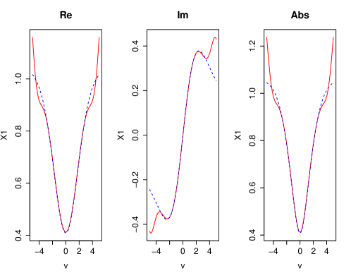
Figure 3: Plots of theoretical (blue dashed) and empirical (red solid) Laplace exponents for Example 2. Graphs present real, imaginary and absolute values. For $v\in[-3,3]$ the curves are visually indistinguishable.

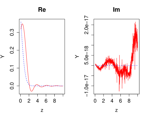
Figure 4: Plots of the Lévy measure (blue dashed line) and its estimate (red solid) depicted for real (left) and imaginary (right) parts. Note that the values on the right plot are quite small.

Next, we proceed with the estimation of the Fourier transform of the measure $\bar{\nu}(x):=e^{-ux}\nu(x)$ of the Lévy measure by applying (25). For the last step of the Algorithm 2, reconstruction of the Lévy measure by (26), we follow [4] and take the so-called flat-top kernel, which is defined as follows:

$$\mathcal{K}(x)=\begin{cases}1,&|x|\leq 0.05,\\ \exp\left(-\frac{e^{-1/(|x|-0.05)}}{1-|x|}\right),&0.05<|x|<1,\\ 0,&|x|\geq 1.\end{cases}$$

The quality of the resulted estimation is given on Figure 4.

5 Theoretical study

Theorem 5.1.

Consider the model (1) with Lévy process $\xi$ in the form (3) satisfying the assumptions (A1) - (A3). Let the sequence $V_{n}$ tend to $\infty$ and moreover satisfy the assumption

$$\Lambda_{n}:=V_{n}\exp\left\{\gamma V_{n}\right\}\sqrt{\log V_{n}}=o\left(\sqrt{\frac{n}{\log(n)}}\right),\;n\to\infty,$$ (33)

where the constant $\gamma$ is introduced in (A2). Then there exists a set $\mathcal{W}_{n}$ such that ${\mathbb{P}}\{\mathcal{W}_{n}\}>1-\alpha n^{-1-\delta}$ (with some positive $\alpha$ and $\delta$) and

$$\mathcal{W}_{n}\subset\Biggl{\{}\sup_{v\in[\varepsilon V_{n},V_{n}]}\left|\hat{\psi}_{n}(u+\mathrm{i}v)-\psi(u+\mathrm{i}v)\right|\leq\beta\>\Lambda_{n}\sqrt{\frac{\log(n)}{n}}\Biggr{\}}$$ (34)

where $\beta>0$ and $u=u^{\circ}$ was introduced in (A2).

Remark 5.2.

The condition (33) fulfills for instance for $V_{n}=\kappa\log(n)$ with $\kappa<1/\left(2\gamma\right)$.

Proof.

1. Denote

$$J(s):=\Bigl{(}\widehat{\mathbb{E}}_{n}\left[A_{\infty}^{s}\right]-{\mathbb{E}}\left[A_{\infty}^{s}\right]\Bigr{)}/{\mathbb{E}}\left[A_{\infty}^{s}\right],$$

where $s=u+\mathrm{i}v$. In this notation,

$$\Biggl{|}\psi(s)-\hat{\psi}_{n}(s)\Biggr{|}=\left|s\Biggl{(}\frac{{\mathbb{E}}\left[A_{\infty}^{s-1}\right]}{{\mathbb{E}}\left[A_{\infty}^{s}\right]}-\frac{\widehat{\mathbb{E}}_{n}\left[A_{\infty}^{s-1}\right]}{\widehat{\mathbb{E}}_{n}\left[A_{\infty}^{s}\right]}\Biggr{)}\right|\\ =\Biggl{|}s\frac{{\mathbb{E}}\left[A_{\infty}^{s-1}\right]}{{\mathbb{E}}\left[A_{\infty}^{s}\right]}\Biggr{|}\;\cdot\;\Biggl{|}\frac{J(s)-J(s-1)}{1+J(s)}\Biggr{|}.$$ (35)

By (12), the first term is equal to $|\psi(s)|$, and therefore by (11) it is bounded by $C_{1}\operatorname{Im}(s)$ for $\operatorname{Im}(s)$ large enough with some $C_{1}>0$. As for the second term, we firstly note that

$$\Biggl{|}\frac{J(s)-J(s-1)}{1+J(s)}\Biggr{|}\leq\frac{|J(s)|+|J(s-1)|}{1-|J(s)|}.$$

The aim of the further proof is to show that the right hand side in the last inequality is bounded by $\sqrt{\log(n)/n}$ on a probability set with desired properties.

2. Proposition 6.2 yields that there exists such set $\mathcal{W}_{n}$ of probability mass larger than $1-\alpha n^{-1-\delta}$, such that it holds on this set

$$\sup_{s:\>\operatorname{Im}(s)\in I_{n}}\Bigl{|}\widehat{\mathbb{E}}_{n}\left[A_{\infty}^{s}\right]-{\mathbb{E}}\left[A_{\infty}^{s}\right]\Bigr{|}\lesssim\sqrt{\log(V_{n})\log(n)/n},\qquad n\to\infty,$$ (36)

where $\alpha$ and $\delta$ are positive, and $I_{n}:=[\varepsilon V_{n},V_{n}]$. In fact, direct application of Proposition 6.2 with a weighting function $w^{*}(x):=\log^{-1/2}\left(e+|x|\right)$ gives

$$\sup_{v\in I_{n}}\Bigl{|}\widehat{\mathbb{E}}_{n}\left[A_{\infty}^{u+\mathrm{i}v}\right]-{\mathbb{E}}\left[A_{\infty}^{u+\mathrm{i}v}\right]\Bigr{|} \leq \sup_{v\in I_{n}}\left[\Bigl{|}\frac{w^{*}(v)}{\inf_{x\in I_{n}}w^{*}(x)}\Bigr{|}\right.$$

$$\left.\hskip 56.9055pt\cdot\Bigl{|}\left(\widehat{{\mathbb{E}}}_{n}\left[A_{\infty}^{u+\mathrm{i}v}\right]-{\mathbb{E}}\left[A_{\infty}^{u+\mathrm{i}v}\right]\right)\Bigr{|}\right]$$

$$\leq \sqrt{\log\left(e+V_{n}\right)}$$

$$\hskip 28.45274pt\cdot\sup_{v\in I_{n}}\Bigl{|}w^{*}(v)\left(\widehat{{\mathbb{E}}}_{n}\left[A_{\infty}^{u+\mathrm{i}v}\right]-{\mathbb{E}}\left[A_{\infty}^{u+\mathrm{i}v}\right]\right)\Bigr{|}$$

$$\lesssim \sqrt{\log(V_{n})\log(n)/n},\qquad n\to\infty.$$

3. Formula (36) in particularly means the following inequlity holds on the set $\mathcal{W}_{n}$

$$\sup_{s:\>\operatorname{Im}(s)\in I_{n}}|J(s)|\lesssim\exp\{\gamma V_{n}\}\;\sqrt{\log(V_{n})\log(n)/n}\qquad n\to\infty,.$$ (37)

It is worth mentioning that under the assumption (33),

$$\sup_{s:\>\operatorname{Im}(s)\in I_{n}}|J(s)|\to 0\quad\mbox{ as }\quad n\to\infty.$$ (38)

Substituting (37) into (35) and taking into account (11) and (38), we arrive at the following bound for the quality of the estimate $\hat{\psi}_{n}(s)$:

$$\Bigl{|}\psi(s)-\hat{\psi}_{n}(s)\Bigr{|}\lesssim V_{n}\exp\{\gamma V_{n}\}\;\sqrt{\log(V_{n})\log(n)/n},$$

which holds on the set $\mathcal{W}_{n}$. This observation completes the proof. ∎

Theorem 5.3.

Consider the setup of Theorem 5.1 and take $V_{n}=\kappa\log(n)$ with $\kappa<1/(2\gamma)$. Then it holds

$$\mathcal{W}_{n}\subset\Biggl{\{}\left|\tilde{c}_{n}-c\right|\leq\frac{\zeta_{1}}{\log^{r+2}(n)}\Biggr{\}}\quad\mbox{and}\quad\mathcal{W}_{n}\subset\Biggl{\{}\left|\tilde{a}_{n}-a\right|\leq\frac{\zeta_{2}}{\log^{r+1}(n)}.\Biggr{\}},$$ (39)

where $s$ is introduced in (A3), the set $\mathcal{W}_{n}$ is defined in Theorem 5.1, and $\zeta_{1},\zeta_{2}>0$.

Proof.

1. First note that the estimate (19) can be rewriten as

$$\tilde{c}_{n}=\int_{0}^{\infty}w_{n}^{*}(v)\operatorname{Im}\hat{\psi}_{n}(u+\mathrm{i}v)dv,\\ \mbox{where}\quad w_{n}^{*}(v)=\frac{w_{n}(v)v}{\int w_{n}(y)y^{2}dy}=\frac{1}{V_{n}^{2}}w^{*}\left(\frac{v}{V_{n}}\right),$$

where $w^{*}(x)=\left(w(x)x\right)/\left(\int w(y)y^{2}dy\right)$. Next, consider the following “theoretical counterpart” of the estimate $\tilde{c}_{n}$:

$$\bar{c}_{n}:=\int_{0}^{\infty}w_{n}^{*}(v)\operatorname{Im}\psi(u+\mathrm{i}v)dv,$$

and note that

$$\left|\hat{c}_{n}-c\right|\leq\left|\hat{c}_{n}-\bar{c}_{n}\right|+\left|\bar{c}_{n}-c\right|.$$ (40)

The first summand in the right hand side of (40) is bounded on the set $\mathcal{W}_{n}$ for $n$ large enough:

$$\left|\hat{c}_{n}-\bar{c}_{n}\right|\leq\ A\>\Lambda_{n}\sqrt{\frac{\log(n)}{n}}\frac{1}{V_{n}},\\ \mbox{where}\quad A:=V_{n}\beta\;\left|\frac{\int w_{n}^{*}(v)vdv}{\int w_{n}^{*}(v)v^{2}dv}\right|=\left|\frac{\int_{\varepsilon}^{1}w^{*}(v)vdv}{\int_{\varepsilon}^{1}w^{*}(v)v^{2}dv}\right|$$ (41)

doesn’t depend on $n$. As for the second term, using $\int w_{n}^{*}(v)vdv=1$, we get

$$\left|\bar{c}_{n}-c\right|=\left|\int_{0}^{\infty}w_{n}^{*}(v)\Bigl{[}\operatorname{Im}\hat{\psi}_{n}(u+\mathrm{i}v)dv-cv\Bigr{]}dv\right|=\left|\int_{0}^{\infty}w_{n}^{*}(v)\operatorname{Im}\mathcal{F}_{\bar{\nu}}(-v)dv\right|.$$

Applying Lemma 6.3 with $w_{n}^{*}(v)=V_{n}^{-2}w_{1}^{*}\left(v/V_{n}\right)$, we get

$$\Bigl{|}\int_{0}^{\infty}w_{n}^{*}(v)\mathcal{F}_{\bar{\nu}}(v)dv\Bigr{|}\lesssim V_{n}^{-(r+2)},\qquad n\to\infty.$$ (42)

Substituting (41) and (42) into (40), and bearing in mind our choice of $V_{n}$, we complete the proof of the first embedding in (39).

2. Without limitations we can assume that $\int_{I\!\!R+}w_{n}(v)dv=\int_{\varepsilon}^{1}w(v)dv=1$. The second embedding directly follows from Theorem 5.1 and the first part of this proof, because

$$\left|\tilde{a}_{n}-a\right| = \left|\left[\int_{I\!\!R_{+}}w_{n}(v)\operatorname{Re}\hat{\psi}_{n}(u+\mathrm{i}v)dv-\tilde{c}_{n}u\right]\right.$$

$$\hskip 42.67912pt\left.-\left[\int_{I\!\!R_{+}}w_{n}(v)\Bigl{(}\operatorname{Re}\psi(u+\mathrm{i}v)+\operatorname{Re}\mathcal{F}_{\bar{\nu}}(-v)\Bigr{)}dv-cu\right]\right|$$

$$\leq \left|\tilde{c}_{n}-c\right|u+\left|\int_{I\!\!R_{+}}w_{n}(v)\Bigl{(}\operatorname{Re}\hat{\psi}_{n}(u+\mathrm{i}v)-\operatorname{Re}\psi(u+\mathrm{i}v)\Bigr{)}dv\right|$$

$$\hskip 113.81102pt+\left|\int_{I\!\!R_{+}}w_{n}(v)\operatorname{Re}\mathcal{F}_{\bar{\nu}}(-v)dv\right|$$

$$\lesssim \frac{\zeta_{1}}{\log^{r+2}(n)}+\beta\>\Lambda_{n}\sqrt{\frac{\log(n)}{n}}+\frac{\lambda}{\log^{r+1}(n)}$$

$$\lesssim \frac{1}{\log^{r+1}(n)},\qquad n\to\infty,$$

where $\lambda>0$. Note that here we use the inequality

$$\left|\int_{I\!\!R_{+}}w_{n}(v)\operatorname{Re}\mathcal{F}_{\bar{\nu}}(-v)dv\right|\lesssim\log^{-(r+1)}(n),$$

which follows by applying Lemma 6.3 to $w_{n}(v)=V_{n}^{-1}w_{n}(v/V_{n})$. This completes the proof. ∎

Theorem 5.4.

Let $\mathscr{A}$ be a set of functions that satisfy assumptions (A1) - (A3). Then it holds

$$\varliminf_{n\to\infty}\inf_{\tilde{c}_{n}^{*}}\sup_{\mathscr{A}}{\mathbb{P}}\Biggl{\{}\left|\tilde{c}_{n}^{*}-c\right|\geq\zeta_{3}\log^{-(r+2)}(n)\Biggr{\}}>0,$$

where $\zeta_{3}$ is some positive constant, the supremum is taken over all models from $\mathscr{A}$, and infimum - over all possible estimates of the parameter $c$.

Proof.

We follow the general reduction scheme, which can be found in [18] and [28]. Consider a class of Lévy processes $\mathscr{A}$ that satisfies the assumptions (A1)-(A3). There exist two Lévy process $\xi_{0}$ and $\xi_{1}$ from $\mathscr{A}$, having Lévy triplets $\left(c_{0},0,\nu_{0}\right)$, $\left(c_{1},0,\nu_{1}\right)$, Laplace exponents $\phi_{0}$, $\phi_{1}$, exponential functionals with densities $p_{0}$, $p_{1}$ and Mellin transforms $M_{0}$, $M_{1}$, such that it holds simultaneously

1. the Lévy triplets are related by the following identities:

   $$c_{0}-c_{1}=2\delta,\qquad\nu_{0}(x)-\nu_{1}(x)=2\delta K^{\prime}_{h}(x),$$ (43)

   where $\delta>0$, $K_{h}(x)=h^{-1}K\left(h^{-1}x\right)$ for any $x\in I\!\!R$ and some $h>0$, and $K\in L^{1}({\mathbb{C}})$ satisfy $\mathcal{F}_{K}(z)=-1$ for $z$ with $\operatorname{Re}(z)\in[-1,1]$ and polynomical decay $\left|F_{K}(z)\right|\lesssim\left|Re(z)\right|^{-\eta}$ as $|z|\to\infty$.

2. the density of one of the functionals, say the first one, decays at most polynomially, i.e., there exists $m\in{\mathbb{N}}$ such that

   $$p_{0}(x)\gtrsim(1+x)^{-2m},\qquad x\to+\infty.$$

3. $M_{0}(s)$ and $M_{1}(s)$ coincide on the lines $s=u^{(k)}+\mathrm{i}v,\>k=1,2,$ for $u^{(1)}=3/2$, $u^{(2)}=m+3/2$, and any $v$. Moreover, the asymptotics of the Mellin transforms along these lines is given by (A2), i.e.,

   $$|M_{j}(u^{(k)}+\mathrm{i}v)|\asymp\exp\{-\gamma^{(k)}|v|\},\qquad\mbox{as}\quad\;v\to\infty,$$

   with some $\gamma^{(k)}>0,\;k=1,2,\>j=0,1.$

Let the exponential functionals of these Lévy processes have distribution laws ${\mathbb{P}}_{0}$ and $P_{1}$.

$$\chi^{2}_{n}(1|0):=\chi^{2}({\mathbb{P}}_{1}^{\otimes n}|{\mathbb{P}}_{0}^{\otimes n})\leq\exp\left\{n\chi^{2}({\mathbb{P}}_{1}|{\mathbb{P}}_{0})\right\}-1,$$

see Lemma 5.5 from [5]. The aim is to show that there exist a constant $C>0$ such that $\chi^{2}_{n}(1|0)<C$; after that the desired result will immediately follow, see Part 2 and especially Theorem 2.2 from [28].

Our choice of the models leads to the following estimate of the chi-squared distance between ${\mathbb{P}}_{1}$ and ${\mathbb{P}}_{2}$:

$$\chi^{2}(1|0):=\chi^{2}({\mathbb{P}}_{1}|{\mathbb{P}}_{0})=\int_{I\!\!R_{+}}\frac{\left(p_{1}(x)-p_{0}(x)\right)^{2}}{p_{0}(x)}\\ \lesssim\int_{I\!\!R_{+}}(1+x^{2m})\left(p_{1}(x)-p_{0}(x)\right)^{2}dx.$$ (44)

By Lemma 6.4 we get that

$$\chi^{2}(1|0)\lesssim\Delta(0)+\Delta(m),\\ \mbox{where}\quad\Delta(\cdot):=\int_{-\infty}^{\infty}\left|M_{0}(\cdot+1/2+\mathrm{i}v)-M_{1}(\cdot+1/2+\mathrm{i}v)\right|^{2}dv.$$ (45)

Note that by (4) and our assumptions,

$$M_{0}(s-1)-M_{1}(s-1)=\frac{\phi_{0}(s)-\phi_{1}(s)}{s}M_{0}(s),$$ (46)

where $s=u^{(k)}+\mathrm{i}v$, $k=1,2$. By our choice of the Lévy measures (43) and the representation of the Laplace exponent (9), we get

$$\phi_{0}(s)-\phi_{1}(s) = \left(c_{0}-c_{1}\right)s+\int_{I\!\!R_{+}}\left(1-e^{-sx}\right)\nu_{0}(dx)$$

$$\hskip 85.35826pt-\int_{I\!\!R_{+}}\left(1-e^{-sx}\right)\nu_{1}(dx)$$

$$= 2\delta s+\int_{I\!\!R_{+}}\left[\nu_{0}(dx)-\nu_{1}(dx)\right]-\left[\mathcal{F}_{\nu_{0}}(\mathrm{i}s)-\mathcal{F}_{\nu_{1}}(\mathrm{i}s)\right]$$

$$= 2\delta s+2\delta\int_{I\!\!R_{+}}K^{\prime}_{h}(x)dx-2\delta\mathcal{F}_{K^{\prime}_{h}}(\mathrm{i}s)$$

Next, we take into account that $\mathcal{F}_{K^{\prime}_{h}}(y)=\mathrm{i}y\mathcal{F}_{K_{h}}(y)=\mathrm{i}yF_{K}(yh)$ for any $y\in{\mathbb{C}}$. Therefore $\int_{I\!\!R_{+}}K^{\prime}_{h}(x)dx=\mathcal{F}_{K^{\prime}_{h}}(0)=0$ and moreover

$$\phi_{0}(s)-\phi_{1}(s)=2\delta s\left(1+\mathcal{F}_{K}(\mathrm{i}sh)\right).$$ (47)

Substituting (47) into (46), we arrive at

$$M_{0}(s-1)-M_{1}(s-1)=2\delta\left(1+\mathcal{F}_{K}(\mathrm{i}sh)\right)M_{0}(s),$$

and therefore

$$\Delta(\cdot)=\delta\int_{I\!\!R}\Bigl{|}1+\mathcal{F}_{K}\Bigl{(}\left(-v+\mathrm{i}u^{(k)}\right)h\Bigr{)}\Bigr{|}^{2}*\Bigl{|}M_{0}\Bigl{(}u^{(k)}+\mathrm{i}v\Bigr{)}\Bigr{|}^{2}dv,$$

where $k=1$ if $\cdot=0$ and $k=2$ if $\cdot=m$. By our assumptions on the kernel $K$, we get

$$\Delta(\cdot)\lesssim\delta\int_{|v|>1/h}e^{-\gamma^{(k)}|v|}dv=\frac{\delta}{\gamma^{(k)}}e^{-\gamma^{(k)}/h},$$

and therefore

$$\chi^{2}(1|0)\lesssim\frac{\delta}{\gamma^{*}}e^{-\gamma^{*}/h},\qquad\mbox{with}\quad\gamma^{*}:=\min\left\{\gamma^{(1)},\gamma^{(2)}\right\}.$$

If we choose $\delta=h^{s+2}$ and $h=\log^{-1}(n)\gamma^{*}/(1+\varepsilon)$ for any (small) $\varepsilon>0$, the $\chi^{2}$ - divergence is bounded by

$$\chi^{2}(1|0)=\frac{\left(\gamma^{*}\right)^{s+2}}{(1+\varepsilon)^{s+2}}\frac{\log^{-(s+2)}(n)}{n^{1+\varepsilon}}\lesssim\frac{\log(C+1)}{n}$$

for any $C>0$ an $n$ large enough. Therefore,

$$\chi^{2}_{n}(1|0)\leq\exp\{n\chi^{2}(1|0)\}-1\leq C,$$

and the statement of the theorem follows.

∎

6 Appendix. Additional proofs

Lemma 6.1 (Exponential inequalities for dependent sequences).

Let $(G_{k},\,k\geq 1)$ be a sequence of centered real-valued random variables on the probability space $(\Omega,\cal F,P)$. Assume that

1. $G_{k}$ is a strongly mixing sequence with the mixing coefficients satisfying

   $$\alpha_{G}(n)\leq\bar{\alpha}_{0}\exp\left\{-\bar{\alpha}_{1}n\right\},\quad n\geq 1,\quad\bar{\alpha}_{0}>0,\quad\bar{\alpha}_{1}>0;$$ (48)

2. $\sup_{k\geq 1}|G_{k}|\leq M$ a.s. for some positive $M$;

3. the quantities

   $$\rho_{k}:={\mathbb{E}}\left[G_{k}^{2}\>\left|2\log G_{k}\right|^{2(1+\varepsilon)}\right],\quad k=1,2,\ldots,$$

   are finite for all $k$ with some small $\varepsilon>0$.

Then there is a positive constant $C_{1}$ depending on $\bar{\alpha}:=\left(\bar{\alpha}_{0},\bar{\alpha}_{1}\right)$ such that

$${\mathbb{P}}\left\{\sum_{k=1}^{n}G_{k}\geq\beta\right\}\leq\exp\left[-\frac{C_{1}\beta^{2}}{nv^{2}+M^{2}+M\beta\log^{2}n}\right].$$

for all $\beta>0$ and $n\geq 4,$ where

$$v^{2}\leq\sup_{k}{\mathbb{E}}[G_{k}^{2}]+C_{2}\sup_{k}\rho_{k}$$

with $C_{2}>0$.

Proof.

The proof directly follows from Theorem A.1 and Corollary A.2 from [6]. ∎

The next result gives the uniform probabilistic inequality for the empirical process. This result is an analogue of Proposition A.3 from [6], which gives the uniform inequality for the case when $u=0$ (see below). For similar results in i.i.d. case, see [25].

Proposition 6.2.

Let $Z_{j},$ $j=1,\ldots,n,$ be a stationary sequence of random variables. Define

$$\varphi_{n}(v) := \frac{1}{n}\sum_{j=1}^{n}\exp\left\{\left(u+\mathrm{i}v\right)Z_{j}\right\},$$

where $u\in I\!\!R_{+}$ is fixed and $v\in I\!\!R$ varies. Let $\varphi(v)$ be a characteristic function of the corresponding stationary distribution. Let also $w$ be a positive monotone decreasing Lipschitz function on $\mathbb{R}_{+}$ such that

$$0<w(z)\leq\frac{1}{\sqrt{\log(e+|z|)}},\quad z\in\mathbb{R}.$$ (49)

Suppose that the following assumptions hold:

(A1)

random variables $e^{Z_{j}}$ possess finite absolute moments of order $p>2$.

(A2)

$Z_{j}$ is a strongly mixing sequence with the mixing coefficients satisfying

$$\alpha_{Z}(n)\leq\bar{\alpha}_{0}\exp\left\{-\bar{\alpha}_{1}n\right\},\quad n\geq 1,\quad\bar{\alpha}_{0}>0,\quad\bar{\alpha}_{1}>0.$$ (50)

Then there are $\delta^{\prime}>0$ and $\zeta_{0}>0$, such that the inequality

$${\mathbb{P}}\left\{\sqrt{\frac{n}{\log n}}\left\|\varphi_{n}-\varphi\right\|_{L_{\infty}(\mathbb{R},w)}>\zeta\right\} \leq B\zeta^{-p}n^{-1-\delta^{\prime}}.$$ (51)

holds for any $\zeta>\zeta_{0}$ and some positive constant $B$ not depending on $\zeta$ and $n.$

Proof.

Denote

$$\mathcal{W}_{n}^{1}(v) := \frac{w(v)}{n}\;\sum_{j=1}^{n}\Bigl{(}e^{(u+\mathrm{i}v)Z_{j}}I\left\{e^{uZ_{j}}<\Xi_{n}\right\}-{\mathbb{E}}\left[e^{(u+\mathrm{i}v)Z}I\left\{e^{uZ}<\Xi_{n}\right\}\right]\Bigr{)},$$

$$\mathcal{W}_{n}^{2}(v) := \frac{w(v)}{n}\;\sum_{j=1}^{n}\Bigl{(}e^{(u+\mathrm{i}v)Z_{j}}I\left\{e^{uZ_{j}}\geq\Xi_{n}\right\}-{\mathbb{E}}\left[e^{(u+\mathrm{i}v)Z}I\left\{e^{uZ}\geq\Xi_{n}\right\}\right]\Bigr{)},$$

where $Z$ is a random variable with stationary distribution of $Z_{j}$. The main idea of the proof is to show that

$${\mathbb{P}}\left\{|\mathcal{W}_{n}^{1}(v)|>\zeta\sqrt{\frac{\log n}{n}}\right\} \leq \widetilde{B}_{1}\zeta^{-p}n^{-1-\delta^{\prime}},$$ (52)

$${\mathbb{P}}\left\{|\mathcal{W}_{n}^{2}(v)|>\zeta\sqrt{\frac{\log n}{n}}\right\} \leq \widetilde{B}_{2}\zeta^{-p}n^{-1-\delta^{\prime}},$$ (53)

with $\Xi_{n}=...$ and some positive $\widetilde{B}_{2}$ and $\widetilde{B}_{2}$.

Step 1. The aim of the first step is to show (52). The proof follows the same lines as the proof of Proposition A.3 from [6].

1.1. Consider the sequence $A_{k}=e^{k},\,k\in\mathbb{N}$ and cover each interval $[-A_{k},A_{k}]$ by $M_{k}=\left(\lfloor 2A_{k}/\gamma\rfloor+1\right)$ disjoint small intervals $\Lambda_{k,1},\ldots,\Lambda_{k,M_{k}}$ of the length $\gamma.$ Let $v_{k,1},\ldots,v_{k,M_{k}}$ be the centers of these intervals. We have for any natural $K>0$

$$\max_{k=1,\ldots,K}\sup_{A_{k-1}<|v|\leq A_{k}}|\mathcal{W}_{n}^{1}(v)|\leq\max_{k=1,\ldots,K}\max_{1\leq m\leq M_{k}}\sup_{v\in\Lambda_{k,m}}|\mathcal{W}_{n}^{1}(v)-\mathcal{W}_{n}^{1}(v_{k,m})|\\ +\max_{k=1,\ldots,K}\max_{\Bigl{\{}\begin{subarray}{c}1\leq m\leq M_{k}:\\ |v_{k,m}|>A_{k-1}\end{subarray}\Bigr{\}}}|\mathcal{W}_{n}^{1}(v_{k,m})|.$$

Hence for any positive $\lambda$,

$${\mathbb{P}}\left(\max_{k=1,\ldots,K}\sup_{A_{k-1}<|v|\leq A_{k}}|\mathcal{W}_{n}^{1}(v)|>\lambda\right)\\ \leq{\mathbb{P}}\left(\sup_{|v_{1}-v_{2}|<\gamma}|\mathcal{W}_{n}^{1}(v_{1})-\mathcal{W}_{n}^{1}(v_{2})|>\lambda/2\right)\\ +\sum_{k=1}^{K}\sum_{\Bigl{\{}\begin{subarray}{c}1\leq m\leq M_{k}:|v_{k,m}|>A_{k-1}\end{subarray}\Bigr{\}}}{\mathbb{P}}(|\mathcal{W}_{n}^{1}(v_{k,m})|>\lambda/2).$$ (54)

The aim of the next two steps is to get the upper bounds for the summands in the right hand side, where $\lambda$ is taken in the form $\lambda=\zeta\sqrt{(\log n)/n}$ with arbitrary large enough $\zeta$.

1.2. We proceed with the first summand in (54). It holds for any $v_{1},v_{2}\in\mathbb{R}$

$$|\mathcal{W}_{n}^{1}(v_{1})-\mathcal{W}_{n}^{1}(v_{2})| \leq \left|w(v_{1})-w(v_{2})\right|\times\max_{v}\left|\frac{\mathcal{W}_{n}^{1}(v)}{w(v)}\right|$$ (55)

$$\cdot\hskip 56.9055pt\left|\frac{\mathcal{W}_{n}^{1}(v_{1})}{w(v_{1})}-\frac{\mathcal{W}_{n}^{1}(v_{2})}{w(v_{2})}\right|\times\max_{v}\left[w(v)\right]$$

$$\leq 2\>\Xi_{n}\left|w(v_{1})-w(v_{2})\right|$$

$$\hskip 14.22636pt+\frac{1}{n}\sum_{j=1}^{n}\Bigl{[}\left|e^{(u+\mathrm{i}v_{1})Z_{j}}-e^{(u+\mathrm{i}v_{2})Z_{j}}\right|I\left\{e^{uZ_{j}}<\Xi_{n}\right\}\Bigr{]}$$

$$\hskip 14.22636pt+\Bigl{|}{\mathbb{E}}\left[\left(e^{(u+\mathrm{i}v_{1})Z}-e^{(u+\mathrm{i}v_{2})Z}\right)I\left\{e^{uZ}<\Xi_{n}\right\}\right]\Bigr{|}$$

$$\leq \left|v_{1}-v_{2}\right|\>\Xi_{n}\>\left[2\>L_{w}+\frac{1}{n}\sum_{j=1}^{n}|Z_{j}|+{\mathbb{E}}|Z|\right],$$

where $L_{\omega}$ is the Lipschitz constant of $w$ and $Z$ is a random variable distributed by the stationary law of the sequence $\left\{Z_{j}\right\}$. Next, the Markov inequality implies

$${\mathbb{P}}\left\{\frac{1}{n}\sum_{j=1}^{n}\Bigl{[}|Z_{j}|-{\mathbb{E}}|Z|\Bigr{]}>c\right\}\leq c^{-p}n^{-p}\>{\mathbb{E}}\left|\sum_{j=1}^{n}\Bigl{[}|Z_{j}|-{\mathbb{E}}|Z|\Bigr{]}\right|^{p}$$

for any $c>0.$ Using now Yokoyama inequality [29] and taking into account the assumptions of the continuity of moments of $Z_{j}$ and the assumption 1 from Lemma 6.1, we get

$${\mathbb{E}}\left|\sum_{j=1}^{n}\Bigl{[}|Z_{j}|-{\mathbb{E}}|Z|\Bigr{]}\right|^{p}\leq C_{p}(\bar{\alpha})n^{p/2},$$

where $C_{p}(\bar{\alpha})$ is some constant depending on $\bar{\alpha}=(\bar{\alpha}_{0},\bar{\alpha}_{1})$ and $p$. Returning to our choice of $\gamma$ and $\lambda$, which in particularly yields that $\gamma=\lambda/\zeta=\sqrt{(\log n)/n},$ we obtain from (55)

$${\mathbb{P}}\Bigl{\{}\sup_{|v_{1}-v_{2}|<\gamma}|\mathcal{W}_{n}^{1}(v_{1})-\mathcal{W}_{n}^{1}(v_{2})|>\lambda/2\Bigr{\}}\leq\\ {\mathbb{P}}\left\{\frac{1}{n}\sum_{j=1}^{n}\Bigl{[}|Z_{j}|-{\mathbb{E}}|Z|\Bigr{]}>\frac{\zeta}{2\Xi_{n}}-2L_{w}-2{\mathbb{E}}|Z|\right\}\\ \leq B_{0}\>c_{p}(\bar{\alpha})\Bigl{(}\zeta/\left(2\Xi_{n}\right)-2L_{w}-2{\mathbb{E}}|Z|\Bigr{)}^{-p}n^{-p/2}\leq B_{1}\zeta^{-p}\>\Xi_{n}^{p}\>n^{-p/2}$$

with some constants $B_{0},B_{1}$ not depending on $\zeta$ and $n,$ provided $\zeta$ is large enough.

1.3. Now we turn to the second term on the right-hand side of (54). Applying Lemma 6.1 with $G_{k}=n\operatorname{Re}\left[\mathcal{W}_{n}^{1}(u_{k,m})\right]$ and $\beta=n\lambda$, we get

$${\mathbb{P}}\left(|\operatorname{Re}\left[\mathcal{W}_{n}^{1}(v_{k,m})\right]|>\lambda/4\right)\leq\mathcal{K},$$

where

$$\mathcal{K}:=\exp\left(-\frac{B_{3}\lambda^{2}n}{B_{2}\Xi_{n}^{2}w^{2}(A_{k-1})\log^{2(1+\varepsilon)}(\Xi_{n}w(A_{k-1}))+\lambda\log^{2}(n)\Xi_{n}w(A_{k-1})}\right)$$

with some constants $B_{2}$ and $B_{3}$ depending only on the characteristics of the process $Z$. Similarly, applying the same result with $G_{k}=n\operatorname{Im}\left[\mathcal{W}_{n}^{1}(u_{k,m})\right]$, we conclude that

$${\mathbb{P}}\left(|\operatorname{Im}\left[\mathcal{W}_{n}^{1}(v_{k,m})\right]|>\lambda/4\right)\leq\mathcal{K},$$

and therefore

$$\sum_{\{|v_{k,m}|>A_{k-1}\}}{\mathbb{P}}(|\mathcal{W}_{n}^{1}(v_{k,m})|>\lambda/2)\leq\left(\lfloor 2A_{k}/\gamma\rfloor+1\right)\mathcal{K}.$$

Set now $\gamma=\sqrt{(\log n)/n}$ and $\lambda=\zeta\sqrt{(\log n)/n}$ and note that under our choice of $\Xi_{n}$,

$$\Xi_{n}^{2}w^{2}(A_{k-1})\log^{2(1+\varepsilon)}(\Xi_{n}w(A_{k-1}))\gtrsim\lambda\log^{2}(n)\Xi_{n}w(A_{k-1}).$$

Therefore,

$$\sum_{\{|v_{k,m}|>A_{k-1}\}}{\mathbb{P}}(|\mathcal{W}_{n}^{1}(v_{k,m})|>\lambda/2)\\ \lesssim A_{k}\sqrt{\frac{n}{\log(n)}}\exp\left(-\frac{B\zeta^{2}\log(n)}{w^{2}(A_{k-1})\Xi_{n}^{2}\log^{2(1+\varepsilon)}(w(A_{k-1}))}\right),\quad n\to\infty$$

with some constant $B>0.$ Fix $\theta>0$ such that $B\theta>1$ and compute

$$\sum_{\{|v_{k,m}|>A_{k-1}\}}{\mathbb{P}}(|\mathcal{W}_{n}^{1}(v_{k,m})|>\lambda/2)\\ \lesssim\sqrt{\frac{n}{\log(n)}}\exp\Bigl{\{}k-\theta B(k-1)-B(k-1)(\zeta^{2}(\log n/\Xi_{n})-\theta)\Bigr{\}}\\ \lesssim\sqrt{\frac{n}{\log(n)}}e^{k(1-\theta B)}e^{-B(k-1)(\zeta^{2}(\log n/\Xi_{n})-\theta)}.$$

Since $\zeta^{2}(\log n/\Xi_{n})>\theta$, we arrive at

$$\sum_{k=2}^{K}\sum_{\{|v_{k,m}|>A_{k-1}\}}{\mathbb{P}}(|\mathcal{W}_{n}(v_{k,m})|>\lambda/2)\\ \lesssim\sqrt{\frac{n}{\log(n)}}e^{-B(\zeta^{2}(\log n/\Xi_{n})-\theta)}\Bigl{[}\sum_{k=2}^{K}e^{k(1-\theta B)}\Bigr{]}\\ \lesssim\log^{-1/2}(n)\exp\Bigl{\{}-B\zeta^{2}(\log n/\Xi_{n})+\log(n)\Bigr{\}}.$$

Taking large enough $\zeta>0$, we get (52).

Step 2. Now we are concentrated on (53). The idea of the proof given below was published in [3], Proposition 7.4.

Consider the sequence

$$R_{n}(v):=\frac{1}{n}\;\sum_{j=1}^{n}e^{(u+\mathrm{i}v)Z_{j}}I\left\{e^{uZ_{j}}\geq\Xi_{n}\right\}.$$

By the Markov inequality we get

$$\left|{\mathbb{E}}\left[R_{n}(u)\right]\right|\leq{\mathbb{E}}\left[e^{uZ_{j}}\right]{\mathbb{P}}\left\{e^{uZ_{j}}\geq\Xi_{n}\right\}\\ \leq\Xi_{n}^{-p}\;\;{\mathbb{E}}\left[e^{uZ_{j}}\right]\;{\mathbb{E}}\left[e^{upZ_{j}}\right]=o\Bigl{(}\sqrt{(\log n)/n}\Bigr{)}$$

Set $\nu_{k}=2^{k},k\in 1,2,...$, then it holds

$$\sum_{k=1}^{\infty}{\mathbb{P}}\Bigl{\{}\max_{j=1..\eta_{k+1}}e^{uZ_{j}}\geq\Xi_{\eta_{k}}\Bigr{\}}\leq\sum_{k=1}^{\infty}\eta_{k+1}{\mathbb{P}}\{e^{uZ}\geq\Xi_{\eta_{k}}\}\\ \leq{\mathbb{E}}e^{puZ}\sum_{k=1}^{\infty}\eta_{k+1}\Xi_{\eta_{k}}^{-p}<\infty.$$

By the Borel-Cantelli lemma,

$${\mathbb{P}}\Bigl{\{}\max_{j=1..\eta_{k+1}}e^{uZ_{j}}\geq\Xi_{\eta_{k}}\quad\mbox{for infinitely many k}\Bigr{\}}=0.$$

From here it follows that $R_{n}(u)-{\mathbb{E}}R_{n}(u)=o\Bigl{(}\sqrt{(\log n)/n}\Bigr{)}$. This completes the proof. ∎

Lemma 6.3.

Let the measure $\bar{\nu}$ be such that $\|\bar{\nu}^{(r)}\|_{\infty}\leq C_{1}$ for some positive $C_{1}$, the weighting function $w_{n}$ admits the property $w_{n}=V_{n}^{-k}w(v/V_{n})$ for some $k>0$ and function $w$ satisfying

$$\|\mathcal{F}_{w(u)/u^{r}}(\cdot)\|_{L_{1}}\leq C_{2}$$

with some $C_{2}>0$. Then

$$\Bigl{|}\int_{0}^{\infty}w_{n}(v)\mathcal{F}_{\bar{\nu}}(v)dv\Bigr{|}\lesssim V_{n}^{-(r+k)},\qquad n\to\infty.$$

Proof.

Following [5], we apply the Plancherel identity:

$$\Bigl{|}\int_{0}^{\infty}w_{n}(v)\mathcal{F}_{\bar{\nu}}(v)dv\Bigr{|} = 2\pi\left|\int_{I\!\!R}\bar{\nu}^{(r)}(x)\overline{\mathcal{F}^{-1}_{w_{n}(\cdot)/(\mathrm{i}\cdot)^{r}}(x)}dx\right|$$

$$\leq 2\pi\>V_{n}^{-(r+k)}\|\bar{\nu}^{(r)}\|_{\infty}\;\|\mathcal{F}_{w(u)/u^{r}}(\cdot)\|_{L_{1}}\lesssim V_{n}^{-(r+k)}.$$

∎

Lemma 6.4 (analogue of the Parseval-Plancherel theorem for Mellin transform).

Let $X_{1}$ and $X_{0}$ be two Lévy process with expontional functionals that have densities $p_{0}$ and $p_{1}$, and Mellin transforms $M_{0}$ and $M_{1}$, resp. For any $b\in I\!\!R$, it holds

$$\int_{0}^{\infty}x^{b}\left(p_{0}(x)-p_{1}(x)\right)^{2}dx\\ =(2\pi)^{-1/2}\int_{-\infty}^{\infty}\left|M_{0}(b/2+1/2+\mathrm{i}v)-M_{1}(b/2+1/2+\mathrm{i}v)\right|^{2}dv.$$

References

- [1] Barndorff-Nielsen, Ole E. and Shiryaev, A.N. Change of Time and Change of Measure. World Scientific, 2010.
- [2] Behme, A. Generalized Ornstein-Uhlenbeck process and extensions. PhD thesis, TU Braunschweig, 2011.
- [3] Belomestny, D. Statistical inference for multidimensional time-changed Lévy processes based on low-frequency data. Arxiv: 1003.0275, 2010.
- [4] Belomestny, D. Statistical inference for time-changed Lévy processes via composite characteristic function estimation. The Annals of Statistics, 39(4):2205–2242, 2011.
- [5] Belomestny, D., and Reiss, M. … In preparation.
- [6] Belomestny, D., Panov V. Abelian theorems for stochastic volatility models with application to the estimation of jump activity. Stochastic Processes and their Applications, 123(1):15–44, 2013.
- [7] Bertoin, J. Lévy processes. Cambridge University Press, 1998.
- [8] Bertoin, J. and Yor, M. Exponential functional of Lévy processes. Probability Surveys, 2:191–212, 2005.
- [9] Carmona, P., Petit, F. and Yor, M. On the distribution and asymptotic results for exponential functionals of Lévy processes. In Exponential functionals and principal values related to Brownian motion, pages 73–130. Bibl. Rev. Mat. Iberoamericana, Madrid, 1997.
- [10] Carmona, P., Petit, F. and Yor, M. Exponential functionals of Lévy processes. In Lévy processes: theory and applicatons, pages 55–59, 1999.
- [11] Comtet, A., Monthus, C., and Yor, M. Exponential functional of Brownain motion and disordered systems. J. Appl. Prob., 35(255-271), 1998.
- [12] Cont, R. and Tankov, P. Financial modelling with jump process. Chapman & Hall, CRC Press UK, 2004.
- [13] Epstein, B. Some applications of the Mellin transform in statistics. The Annals of Mathematical Statistics, 19(3):370–379, 1948.
- [14] Erickson, K. and Maller, A. Convergence of Lévy integrals. In Émery M, Ledoux, M, and Yor,M., editor, Séminaire de probabilités 38. Springer, 2005.
- [15] Guillemin, F., Robert, P., and Zwart, B. AIMD algorithms and exponential functionals. The Annals of Applied Probability., 14(1):90–117, 2004.
- [16] Kawata, T. Fourier analysis in probability theory. Academic Press, 1972.
- [17] Klüppelberg, C., Lindner, A., and Maller, R. A continuous-time GARCH process driven by a Lévy process: stationarity and second-order behaviour. J. Appl. Prob., 41:601–622, 2004.
- [18] Korostelev, A. and Tsybakov, A. Minimax theory of image reconstruction. Lecture notes in Statistics 82. New York: Springer, 1993.
- [19] Kuznetsov, A. On the distribution of exponential functionals for Lévy processes with jumps of rational transform. Stochastic Processes and their Applications, 122:654–663, 2012.
- [20] Kuznetsov, A., Pardo, J.C., and Savov, V. Distributional properties of exponential functionals of Lévy processes. arxiv:1106.6365v1, 2011.
- [21] Litvak, N. and Adan, I. The travel time in carousel systems under the nearest item heuristic. J. Appl. Prob., 38:45–54, 2001.
- [22] Litvak, N. and van Zwet, W. On the minimal travel time needed to collect items on a circle. J. Appl. Prob., 14(2):881–902, 2004.
- [23] Maulik, K. and Zwart, B. Tail asymptotics for exponential functionals of Lévy processes. Stochastic Process. Appl., 116:156–177, 2006.
- [24] Monthus, C. Etude de quelques fonctionnelles du mouvement Brownien et de certaines propriétés de la diffusion unidimensionnelle en milieu aléatoire. PhD thesis, Université Paris VI, 1995.
- [25] Neumann, M., and Reiss, M. Nonparametric estimation for Lévy processes from low-frequency observations. Bernoulli, 15(1):223–248, 2009.
- [26] Sato, K. Lévy processes and infinitely divisible distributions. Cambridge University Press, Cambridge University Press, 1999.
- [27] Schoutens, W. Lévy processes in finance. John Wiley and Sons, 2003.
- [28] Tsybakov, A. Introduction to nonparametric estimation. Springer, New York, 2009.
- [29] Yokoyama, R. Moment bounds for stationary mixing sequences. Zeitschrift für Wahrscheinlichkeitstheorie und Verw. Gebiete, 52(45-57), 1980.
- [30] Yor, M. Exponential functional of Brownain motion and related processes. Springer., 2001.