The Bernstein Function: A Unifying Framework of Nonconvex Penalization in Sparse Estimation

Abstract

In this paper we study nonconvex penalization using Bernstein functions. Since the Bernstein function is concave and nonsmooth at the origin, it can induce a class of nonconvex functions for high-dimensional sparse estimation problems. We derive a threshold function based on the Bernstein penalty and give its mathematical properties in sparsity modeling. We show that a coordinate descent algorithm is especially appropriate for penalized regression problems with the Bernstein penalty. Additionally, we prove that the Bernstein function can be defined as the concave conjugate of a $\varphi$-divergence and develop a conjugate maximization algorithm for finding the sparse solution. Finally, we particularly exemplify a family of Bernstein nonconvex penalties based on a generalized Gamma measure and conduct empirical analysis for this family.

Keywords: nonconvex penalization, Bernstein functions, coordinate descent algorithms, the generalized Gamma measure, $\varphi$-divergences, conjugate maximization algorithms

1 Introduction

Variable selection plays a fundamental role in statistical modeling for high-dimensional data sets, especially when the underlying model has a sparse representation. The approach based on penalty theory has been widely used for variable selection in the literature. A principled approach is due to the lasso of Tibshirani (1996), which employs the $\ell_{1}$-norm penalty and performs variable selection via the soft threshold operator. However, Fan and Li (2001) pointed out that the lasso shrinkage method produces biased estimates for the large coefficients. Zou (2006) argued that the lasso might not be an oracle procedure under certain scenarios.

Accordingly, Fan and Li (2001) proposed three criteria for a good penalty function. That is, the resulting estimator should hold sparsity, continuity and unbiasedness. Moreover, Fan and Li (2001) showed that a nonconvex penalty generally admits the oracle properties. This leads to recent developments of nonconvex penalization in sparse learning. There exist many nonconvex penalties, including the $\ell_{q}$ ($q\in(0,1)$) penalty, the smoothly clipped absolute deviation (SCAD) (Fan and Li, 2001), the minimax concave plus penalty (MCP) (Zhang, 2010a), the kinetic energy plus penalty (KEP) (Zhang et al., 2013b), the capped-$\ell_{1}$ function (Zhang, 2010b, Zhang and Zhang, 2012), the nonconvex exponential penalty (EXP) (Bradley and Mangasarian, 1998, Gao et al., 2011), the LOG penalty (Mazumder et al., 2011, Armagan et al., 2013), etc. These penalties have been demonstrated to have attractive properties theoretically and practically.

On one hand, nonconvex penalty functions typically have the tighter approximation to the $\ell_{0}$-norm and hold the oracle properties (Fan and Li, 2001). On the other hand, they would yield computational challenges due to nondifferentiability and nonconvexity. Recently, Mazumder et al. (2011) developed a SparseNet algorithm base on coordinate descent. Especially, the authors studied the coordinate descent algorithm for the MCP function (also see Breheny and Huang, 2010). Moreover, Mazumder et al. (2011) proposed some desirable properties for threshold operators based on nonconvex penalties. For example, the threshold operator should be a strict nesting w.r.t. a sparsity parameter. However, the authors claimed that not all nonconvex penalties are suitable for use with coordinate descent.

In this paper we introduce Bernstein functions into sparse estimation, giving rise to a unifying approach to nonconvex penalization. The Bernstein function is a class of functions whose first-order derivatives are completely monotone (Schilling et al., 2010, Feller, 1971). The Bernstein function can be formed as a class of sparsity-inducing nonconvex penalty functions. Moreover, the Bernstein function has the Lévy-Khintchine representation. We particularly exemplify a family of Bernstein nonconvex penalties based on a generalized Gamma measure (Aalen, 1992, Brix, 1999). The special cases include the KEP, nonconvex LOG and EXP as well as a penalty function that we call linear-fractional (LFR) function. Moreover, we find that the MCP function is a truncated special version.

The Bernstein function has attractive ability in sparsity modeling. Geometrically, the Bernstein function holds the property of regular variation (Feller, 1971). That is, the Bernstein function bridges the $\ell_{q}$-norm ($0\leq q<1$) and the $\ell_{1}$-norm. Theoretically, it admits the oracle properties and can results in a unbiased and continuous sparse estimator. Computationally, the resulting estimation problem can be efficiently solved by using coordinate descent algorithms. Moreover, the corresponding threshold operator has to some extend the nesting property (Mazumder et al., 2011).

Another important contribution of this paper offers a new construction approach for Bernstein functions. That is, we show that the Bernstein function can be be defined as concave conjugates of $\varphi$-divergences (Csiszár, 1967, Censor and Zenios, 1997) under certain conditions. This construction illustrates an interesting connection between LOG and EXP as well as between KEP and MCP (Zhang and Tu, 2012, Zhang et al., 2013b). We note that Wipf and Nagarajan (2008) used the idea of concave conjugate for expressing the automatic relevance determination (ARD) cost function, and Zhang (2010b) derived the bridge penalty by using the idea of concave conjugate. To the best of our knowledge, however, our work is the first time to uncover the intrinsic connection between the Bernstein function and the $\varphi$-divergence.

Based on this new construction approach, we also develop a conjugate-maximization (CM) algorithm for solving penalized regression problems. The CM algorithm consists of a C-step and an M-step. There is an interesting resemblance between CM and EM. The C-step of CM calculates the concave conjugate of a $\varphi$-divergence with respect to an auxiliary (weight) vector, while the E-step of EM the expected sufficient statistics with respect to missing data. The M-steps of both CM and EM are to find the new estimate of the parameter vector in question. Additionally, the CM algorithm shares the same convergence property with the conventional EM algorithm (Wu, 1983).

It is worth pointing out that the CM algorithm is related to the augmented Lagrangian method (Nocedal and Wright, 2006, Censor and Zenios, 1997). Additionally, the CM algorithm enjoys the idea behind the iterative reweighted $\ell_{2}$ or $\ell_{1}$ methods (Chartrand and Yin, 2008, Candès et al., 2008, Wipf and Nagarajan, 2008, Daubechies et al., 2010, Wipf and Nagarajan, 2010, Zhang, 2010b). Thus, CM also implies a so-called majorization-minimization (MM) procedure (Hunter and Li, 2005). An attractive merit of the CM over the existing MM methods is its ability in handling the choice of tuning parameters, which is a very important issue in nonconvex sparse regularization.

The remainder of this paper is organized as follows. Section 2 exploits Bernstein functions in the construction of nonconvex penalties. In Section 3 we investigate sparse estimation problems based on the Bernstein function and devise the coordinate descent algorithm for finding the sparse solution. In Section 4 we conduct theoretical analysis of the corresponding sparse estimation problem. In Section 5 we study Bernstein penalty functions based on concave conjugate of the $\varphi$-divergence. In Section 6 we devise the CM algorithm based on the the $\varphi$-divergence. Finally, we conclude our work in Section 7.

2 Nonconvex Penalization via Bernstein Functions

Suppose we are given a set of training data $\{({\bf x}_{i},y_{i}):i=1,\ldots,n\}$, where the ${\bf x}_{i}\in{\mathbb{R}}^{p}$ are the input vectors and the $y_{i}$ are the corresponding outputs. Moreover, we assume that $\sum_{i=1}^{n}{\bf x}_{i}={\bf 0}$ and $\sum_{i=1}^{n}y_{i}=0$. We now consider the following linear regression model:

$${\bf y}={\bf X}{\bf b}+\mbox{\boldmath$\varepsilon$\unboldmath},$$

where ${\bf y}=(y_{1},\ldots,y_{n})^{T}$ is the $n{\times}1$ output vector, ${\bf X}=[{\bf x}_{1},\ldots,{\bf x}_{n}]^{T}$ is the $n{\times}p$ input matrix, and $\varepsilon$ is a Gaussian error vector $N(\mbox{\boldmath$\varepsilon$\unboldmath}|{\bf 0},\sigma{\bf I}_{n})$. We aim to find a sparse estimate of regression vector ${\bf b}=(b_{1},\ldots,b_{p})^{T}$ under the regularization framework.

The classical regularization approach is based on a penalty function of ${\bf b}$. That is,

$$\min_{{\bf b}}\;\Big{\{}F(b)\triangleq\frac{1}{2}\|{\bf y}{-}{\bf X}{\bf b}\|_{2}^{2}+P({\bf b};\lambda)\Big{\}},$$

where $P(\cdot)$ is the regularization term penalizing model complexity and $\lambda$ ($>0$) is the tuning parameter of balancing the relative significance of the loss function and the penalty.

A widely used setting for penalty is $P({\bf b};\lambda)=\sum_{j=1}^{p}P(b_{j};\lambda)$, which implies that the penalty function consists of $p$ separable subpenalties. In order to find a sparse solution of ${\bf b}$, one imposes the $\ell_{0}$-norm penalty $\|{\bf b}\|_{0}$ to ${\bf b}$ (i.e., the number of nonzero elements of ${\bf b}$). However, the resulting optimization problem is usually NP-hard. Alternatively, the $\ell_{1}$-norm $\|{\bf b}\|_{1}=\sum_{j=1}^{p}|b_{j}|$ is an effective convex penalty. Recently, some nonconvex alternatives, such as the log-penalty, SCAD, MCP and KEP, have been employed. Meanwhile, iteratively reweighted $\ell_{q}$ ($q=1$ or $2$) minimization or coordination descent methods were developed for finding sparse solutions.

In this paper we are concerned with nonconvex penalization based on a Bernstein function (Schilling et al., 2010). Let $f\in C^{\infty}(0,\infty)$ with $f\geq 0$. We say $f$ is completely monotone if $(-1)^{k}f^{(k)}\geq 0$ for all $k\in{\mathbb{N}}$ and a Bernstein function if $(-1)^{k}f^{(k)}\leq 0$ for all $k\in{\mathbb{N}}$. It is well known that $f$ is a Bernstein function if and only if the mapping $s\mapsto\exp(-tf(s))$ is completely monotone for all $t\geq 0$. Additionally, $f$ is a Bernstein function if and only if it has the representation

$$f(s)=a+\beta s+\int_{0}^{\infty}{\big{[}1-\exp(-su)\big{]}\nu(du)}\;\mbox{ for all }s>0,$$

where $a,\beta\geq 0$, and $\nu$ is the Lévy measure satisfying additional requirements $\nu(-\infty,0)=0$ and $\int_{0}^{\infty}{\min(u,1)\nu(du)}<\infty$. Moreover, this representation is unique. The representation is famous as the Lévy-Khintchine formula.

Since $\mathop{\lim}\limits_{s\to 0}f(s)=a$ and $\mathop{\lim}\limits_{s\to\infty}\frac{f(s)}{s}=\beta$ (Schilling et al., 2010), we will assume that $\mathop{\lim}\limits_{s\to 0}f(s)=0$ and $\mathop{\lim}\limits_{s\to\infty}\frac{f(s)}{s}=0$ to make $a=0$ and $\beta=0$. Note that $s^{q}$ for $q\in(0,1)$ is a Bernstein function of $s$ on $(0,\infty)$ satisfying the above assumptions. However, $f(s)=s$ is Bernstein but does not satisfy the condition $\mathop{\lim}\limits_{s\to\infty}\frac{f(s)}{s}=0$. Indeed, $f(s)=s$ is an extreme case because $\beta=1$ and $\nu(du)=\delta_{0}(u)du$ (the Dirac Delta measure) in its Lévy-Khintchine formula. In fact, the condition $\mathop{\lim}\limits_{s\to\infty}\frac{f(s)}{s}=0$ aims to exclude this Bernstein function for our concern in this paper.

2.1 Bernstein Penalty Functions

We now define the penalty function $P({\bf b};\lambda)$ as $\lambda\sum_{j=1}^{p}\Phi(|b_{j}|)$, where the penalty term $\Phi(s)$ is a Bernstein function of $s$ on $(0,\infty)$ such that $\mathop{\lim}\limits_{s\to 0}\Phi(s)=0$ and $\mathop{\lim}\limits_{s\to\infty}\frac{\Phi(s)}{s}=0$. Clearly, $\Phi(s)$ is nonnegative, nondecreasing and concave on $(0,\infty)$, because $\Phi(s)\geq 0$, $\Phi^{\prime}(s)\geq 0$ and $\Phi{{}^{\prime\prime}}(s)\leq 0$. Moreover, we have the following theorem.

Theorem 1

Let $\Phi(s)$ be a nonzero Bernstein function of $s$ on $(0,\infty)$. Assume $\mathop{\lim}\limits_{s\to 0}\Phi(s)=0$ and $\mathop{\lim}\limits_{s\to\infty}\frac{\Phi(s)}{s}=0$. Then

1. $\Phi(|b|)$ is a nonnegative and nonconvex function of $b$ on $(-\infty,\infty)$, and an increasing function of $|b|$ on $[0,\infty)$.

2. $\Phi(|b|)$ is continuous w.r.t. $b$ but nondifferentiable at the origin.

Recall that under the conditions in Theorem 1, $a$ and $\beta$ in the Lévy-Khintchine formula vanish. Theorem 1 (b) shows that $\Phi^{\prime}(|b|)$ is singular at the origin. Thus, $\Phi(|b|)$ can define a class of sparsity-inducing nonconvex penalty functions. We can clearly see the connection of the bridge penalty $|b|^{\rho}$ with the $\ell_{0}$-norm and the $\ell_{1}$-norm as $\rho$ goas from $0$ to 1. However, the sparse estimator resulted from the bridge penalty is not continuous. This would make numerical computations and model predictions unstable (Fan and Li, 2001). In this paper we consider another class of Bernstein nonconvex penalties.

In particular, to explore the relationship of the Bernstein penalties with the $\ell_{0}$-norm and the $\ell_{1}$-norm, we further assume that $\mathop{\lim}\limits_{s\to 0}\Phi^{\prime}(s)<\infty$. Since $\Phi(s)$ is a nonzero Bernstein function of $s$, we can conclude that $\Phi^{\prime}(0)>0$. If it is not true, we have $\Phi^{\prime}(s)=0$ due to $\Phi^{\prime}(s)\leq\Phi^{\prime}(0)$. This implies that $\Phi(s)=0$ for any $s\in(0,\infty)$ because $\Phi(0)=0$. This conflicts with that $\Phi(s)$ is nonzero. Similarly, we can also deduce $\Phi{{}^{\prime\prime}}(0)<0$. Based on this fact, we can change the assumption $\Phi^{\prime}(0)<\infty$ as $\Phi^{\prime}(0)=1$ without loss of generality. In fact, we can replace $\Phi(s)$ with $\frac{\Phi(s)}{\Phi^{\prime}(0)}$ to met this assumption, because the resulting $\Phi(s)$ is still Bernstein and satisfies $\Phi(0)=0$, $\mathop{\lim}\limits_{s\to\infty}\frac{\Phi(s)}{s}=0$ and $\Phi^{\prime}(0)=1$.

Theorem 2

Assume the conditions in Theorem 1 hold. If $\Phi^{\prime}(0)=\mathop{\lim}\limits_{s\to 0}\Phi^{\prime}(s)=1$, then

$$\lim_{\alpha\to 0+}\frac{\Phi(\alpha|b|)}{\Phi(\alpha)}=|b|.$$

Furthermore, if $\mathop{\lim}\limits_{s\to\infty}\frac{{s\Phi^{\prime}(s)}}{\Phi(s)}$ exists, then for $b\neq 0$,

$$\lim_{\alpha\to\infty}\frac{\Phi(\alpha|b|)}{\Phi(\alpha)}=|b|^{\gamma},$$

where $\gamma=\mathop{\lim}\limits_{s\to\infty}\frac{{s\Phi^{\prime}(s)}}{\Phi(s)}\in[0,1)$. Especially, if $\gamma\in(0,1)$, we also have

$$\lim_{\alpha\to\infty}\frac{\Phi^{\prime}(\alpha|b|)}{\Phi^{\prime}(\alpha)}=|b|^{\gamma{-}1}.$$

Remarks 1

It is worth noting that $\Phi^{\prime}(s)$ is completely monotone on $(0,\infty)$. Moreover, $\Phi^{\prime}(s)$ is the Laplace transform of some probability distribution due to $\Phi^{\prime}(0)=1$ (Feller, 1971). Additionally, Lemma 15 (see the appendix) shows that $\mathop{\lim}\limits_{s\to\infty}\frac{{s\Phi^{\prime}(s)}}{\Phi(s)}=0$ whenever $\mathop{\lim}\limits_{s\to\infty}\Phi(s)<\infty$. If $\mathop{\lim}\limits_{s\to\infty}\Phi(s)=\infty$, we take $\Psi(s)\triangleq\log(1+\phi(s))$ which is also Bernstein and holds the conditions $\Psi(0)=0$, $\Psi^{\prime}(0)=1$ and $\Psi^{\prime}(\infty)=0$. In this case, consider $\Psi^{\prime}(s)=\frac{\Phi^{\prime}(s)}{1+\Phi(s)}$ and $\mathop{\lim}\limits_{s\to\infty}\frac{{s\Phi^{\prime}(s)}}{\Phi(s)}=\mathop{\lim}\limits_{s\to\infty}s\Psi^{\prime}(s)$. Thus, Lemma  15-(b) directly applies the Bernstein function $\Psi(s)$. In summary, the condition “$\mathop{\lim}\limits_{s\to\infty}\frac{{s\Phi^{\prime}(s)}}{\Phi(s)}$ exists” is essentially natural.

Remarks 2

It follows from Theorem 1 in Chapter VIII.9 of Feller (1971) that $\mathop{\lim}\limits_{s\to\infty}\frac{{s\Phi^{\prime}(s)}}{\Phi(s)}=\gamma\in(0,1)$ if and only if $\mathop{\lim}\limits_{\alpha\to\infty}\frac{\Phi^{\prime}(\alpha|b|)}{\Phi^{\prime}(\alpha)}=|b|^{\gamma{-}1}$. However, $\mathop{\lim}\limits_{\alpha\to\infty}\frac{\Phi^{\prime}(\alpha|b|)}{\Phi^{\prime}(\alpha)}=|b|^{{-}1}$ (i.e., $\gamma=0$) is only sufficient for $\mathop{\lim}\limits_{s\to\infty}\frac{{s\Phi^{\prime}(s)}}{\Phi(s)}=0$. It is also seen from Lemma 17 in the appendix that $\mathop{\lim}\limits_{s\to\infty}\frac{\Phi(s)}{\log(s)}<\infty$ is a sufficient condition for $\mathop{\lim}\limits_{s\to\infty}\frac{{s\Phi^{\prime}(s)}}{\Phi(s)}=0$ and from Lemma 18 in the appendix that $\mathop{\lim}\limits_{s\to\infty}\frac{{s\Phi^{\prime}(s)}}{\Phi(s)}=\gamma\in[0,1)$.

The second part of Theorem 2 shows that the property of regular variation for the Bernstein function $\Phi(s)$ and its derivative $\Phi^{\prime}(s)$ (Feller, 1971). That is, $\Phi(s)$ and $\Phi^{\prime}(s)$ vary regularly with exponents $\gamma$ and $\gamma{-}1$, respectively. If $\mathop{\lim}\limits_{s\to\infty}\frac{\Phi(s)}{\log(s)}<\infty$, then $\Phi(s)$ varies slowly (i.e., $\gamma=0$). This property implies an important connection of the Bernstein function with the $\ell_{0}$-norm and $\ell_{1}$-norm. With this connection, we see that $\alpha$ plays a role of sparsity parameter because it measures sparseness of $\Phi(\alpha|{\bf b}|)/\Phi(\alpha)$. In the following we present a family of Bernstein functions which admit the properties in Theorem 2.

Table 1: Several Bernstein functions $\Phi_{\rho}(s)$ on $[0,\infty)$ as well as their derivatives

	Bernstein functions	First-order derivatives	Lévy measures
KEP	$\Phi_{-1}(s)=\sqrt{2s{+}1}-1$	$\Phi_{-1}^{\prime}(s)=\frac{1}{\sqrt{2s+1}}$	$\nu(du)=\frac{1}{\sqrt{2\pi}}u^{{-}\frac{3}{2}}\exp({-}\frac{u}{2})du$
LOG	$\Phi_{0}(s)=\log\big{(}s{+}1\big{)}$	$\Phi_{0}^{\prime}(s)=\frac{1}{s{+}1}$	$\nu(du)=\frac{1}{u}\exp({-}{u})du$
LFR	$\Phi_{{1}/{2}}(s)=\frac{2s}{s+2}$	$\Phi^{\prime}_{{1}/{2}}(s)=\frac{4}{({s}+{2})^{2}}$	$\nu(du)={4}\exp(-{2u})du$
EXP	$\Phi_{1}(s)=1-\exp(-s)$	$\Phi_{1}^{\prime}(s)=\exp(-s)$	$\nu(du)=\delta_{1}(u)du$

2.2 Examples

We consider a family of Bernstein functions of the form

$$\Phi_{\rho}(s)=\left\{\begin{array}[]{ll}\log(1+s)&\mbox{if }\rho=0,\\ \frac{1}{\rho}\Big{[}1-\big{(}1+{(1{-}\rho)}s\big{)}^{-\frac{\rho}{1-\rho}}\Big{]}&\mbox{if }\rho<1\mbox{ and }\rho\neq 0,\\ 1-\exp(-s)&\mbox{if }\rho=1.\end{array}\right.$$ (1)

It can be directly verified that $\Phi_{0}(s)=\mathop{\lim}\limits_{\rho\to 0}\Phi_{\rho}(s)$ and $\Phi_{1}(s)=\mathop{\lim}\limits_{\rho\to 1-}\Phi_{\rho}(s)$. The corresponding Lévy measure is

$$\nu(du)=\frac{((1{-}\rho))^{-1/(1{-}\rho)}}{\Gamma(1/(1{-}\rho))}u^{\frac{\rho}{1-\rho}-1}\exp\Big{(}{-}\frac{u}{(1{-}\rho)}\Big{)}du.$$ (2)

Note that ${u}\nu(du)$ forms a Gamma measure for random variable $u$. Thus, this Lévy measure $\nu(du)$ is referred to as a generalized Gamma measure (Brix, 1999). This family of the Bernstein functions were studied by Aalen (1992) for survival analysis. We here show that they can be also used for sparsity modeling.

It is easily seen that the Bernstein functions $\Phi_{\rho}(s)$ for $\rho\leq 1$ satisfy the conditions: $\Phi(0)=0$, $\Phi^{\prime}(0)=1$ and $(-1)^{k}\Phi^{(k+1)}(0)<\infty$ for $k\in{\mathbb{N}}$, in Theorem 2 and Lemma 15 (see the appendix). Thus, $\Phi_{\rho}(s)$ for $\rho\leq 1$ have the properties given in Theorem 2 and Lemma 15. These properties show that when letting $s=|b|$, the Bernstein functions $\Phi(|b|)$ form nonconvex penalties.

The derivative of $\Phi_{\rho}(s)$ is defined by

$$\Phi^{\prime}_{\rho}(s)=\left\{\begin{array}[]{ll}\frac{1}{1{+}s}&\mbox{if }\rho=0,\\ \big{(}1+{(1{-}\rho)}s\big{)}^{-\frac{1}{1-\rho}}&\mbox{if }\rho<1\mbox{ and }\rho\neq 0,\\ \exp(-s)&\mbox{if }\rho=1.\end{array}\right.$$ (3)

It is also directly verified that $\Phi^{\prime}_{0}(s)=\mathop{\lim}\limits_{\rho\to 0}\Phi^{\prime}_{\rho}(s)$ and $\Phi^{\prime}_{1}(s)=\mathop{\lim}\limits_{\rho\to 1-}\Phi^{\prime}_{\rho}(s)$. When $\rho\in[0,1]$, we have $\mathop{\lim}\limits_{s\to\infty}\frac{s\Phi^{\prime}_{\rho}(s)}{\Phi_{\rho}(s)}=0$ (or $\mathop{\lim}\limits_{s\rightarrow\infty}\frac{\Phi(s)}{\log(s)}<\infty$). When $\rho<0$, we then have $\mathop{\lim}\limits_{s\to\infty}\frac{s\Phi^{\prime}_{\rho}(s)}{\Phi_{\rho}(s)}=\frac{\rho}{\rho{-}1}\in(0,1)$.

Proposition 3

Let $\Phi_{\rho}(s)$ on $(0,\infty)$ be defined in (1). Then

1. If $-\infty<\rho_{1}<\rho_{2}\leq 1$ then $\Phi^{\prime}_{\rho_{1}}(s)\geq\Phi^{\prime}_{\rho_{2}}(s)$ and $\Phi_{\rho_{1}}(s)\geq\Phi_{\rho_{2}}(s)$;

2. $\mathop{\lim}\limits_{\alpha\to\infty}\frac{\Phi^{\prime}_{\rho}(\alpha)}{\alpha^{\gamma-1}}=(1-\gamma)^{1-\gamma}$ where $\gamma=0$ if $\rho\in(0,1]$ and $\gamma=\frac{\rho}{\rho{-}1}$ if $\rho\in(-\infty,0]$, and

   $$\mathop{\lim}\limits_{\alpha\to\infty}\frac{\Phi_{\rho}(\alpha s)}{\Phi_{\rho}(\alpha)}=\left\{\begin{array}[]{ll}1&\mbox{if }\rho\in[0,1],\\ s^{\frac{\rho}{\rho{-}1}}&\mbox{if }\rho\in(-\infty,0).\end{array}\right.$$

Proposition 3-(b) shows the property of regular variation for $\Phi_{\rho}(s)$; that is, $\Phi_{\rho}(s)$ varies slowly when $0\leq\rho\leq 1$, while it varies regularly with exponent $\rho/(\rho{-}1)$ when $\rho<0$. Thus, $\frac{\Phi_{\rho}(\alpha|b|)}{\Phi_{\rho}(\alpha)}$ for $\rho<0$ approaches to the $\ell_{\rho/(\rho{-}1)}$-norm $\|b\|_{\rho/(\rho{-}1)}$ as $\alpha\to\infty$.

We list four special Bernstein functions in Table 1 by taking different $\rho$. Specifically, these penalties are the kinetic energy plus (KEP) function, nonconvex log-penalty (LOG), nonconvex exponential-penalty (EXP), and linear-fractional (LFR) function, respectively. Figure 1 depicts these functions and their derivatives. In Table 1 we also give the Lévy measures corresponding to these functions. Clearly, KEP gets a continuum of penalties from $\ell_{1/2}$ to the $\ell_{1}$, as varying $\alpha$ from $\infty$ to $0$ (Zhang et al., 2013b). But the LOG, EXP and LFR penalties get the entire continuum of penalties from $\ell_{0}$ to the $\ell_{1}$. The LOG, EXP and LFR penalties have been applied in the literature (Bradley and Mangasarian, 1998, Gao et al., 2011, Weston et al., 2003, Geman and Reynolds, 1992, Nikolova, 2005). In image processing and computer vision, these functions are usually also called potential functions. However, to the best of our knowledge, there is no work to establish their connection with Bernstein functions.

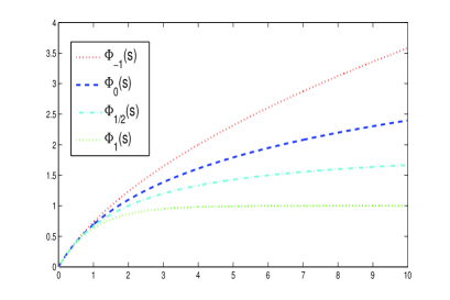
(a) $\Phi_{\rho}(s)$

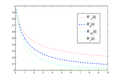
(b) $\Phi^{\prime}_{\rho}(s)$

Figure 1: (a) The Bernstein functions $\Phi_{\rho}(s)$ for $\rho=-1$, $\rho=0$, $\rho=\frac{1}{2}$ and $\rho=1$ corresponding to KEP, LOG, LFR and EXP. (b) The corresponding derivatives $\Phi^{\prime}_{\rho}(s)$.

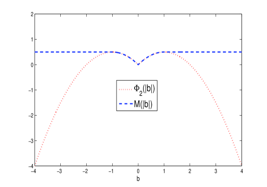
Figure 2: The Bernstein function $\Phi_{2}(|b|)$ and the MCP function $M(|b|)$.

Finally, we note that the MCP function can be regarded as a truncated version of $\Phi_{2}(s)$ (i.e., $\rho=2$). Clearly, $\Phi_{2}(s)$ is well-defined for $s\geq 0$ but no longer Bernstein, because $\Phi_{2}(s)$ is negative when $s>2$. Moreover, it is decreasing when $s\geq 1$ (see Figure 2). To make a concave penalty function from $\Phi_{2}(s)$, we truncate $\Phi_{2}(s)$ as $1/2$ whenever $s\geq 1$, yielding the MCP function. That is,

$$M(\alpha s)=\left\{\begin{array}[]{ll}\frac{1}{2}&\mbox{ if }s\geq\frac{1}{\alpha},\\ \alpha s-\frac{\alpha^{2}s^{2}}{2}&\mbox{ if }s<\frac{1}{\alpha}.\end{array}\right.$$ (4)

3 Sparse Estimation Based on Bernstein Penalty Functions

We now study mathematical properties of the sparse estimators based on Bernstein penalty functions. These properties show that Bernstein penalty functions are suitable for use of a coordinate descent algorithm (Mazumder et al., 2011).

3.1 Threshold Operators

Let $\Phi(|b|)$ be a Bernstein penalty function. Following Fan and Li (2001), we define the univariate penalized least squares problem

$$J_{1}(b)\triangleq\frac{1}{2}(z-b)^{2}+{\lambda}\Phi(|b|),$$ (5)

where $z={\bf x}^{T}{\bf y}$. Fan and Li (2001) stated that a good penalty should result in an estimator with three properties. (a) “Unbiasedness:” it is nearly unbiased when the true unknown parameter is large; (b) “Sparsity:” it is a threshold rule, which automatically sets small estimated coefficients to zero; (c) “Continuity:” it is continuous in $z$ to avoid instability in model computation and prediction.

According to the discussion in Fan and Li (2001), the resulting estimator from (5) is nearly unbiased if $\Phi^{\prime}(|b|)\rightarrow 0$ as $|b|\rightarrow\infty$. The Bernstein penalty function satisfies the conditions $\Phi(0+)=0$ and $\mathop{\lim}\limits_{s\to\infty}\Phi^{\prime}(s)=0$, so it can result in an unbiased sparse estimator.

Theorem 4

Let $\Phi(s)$ be a nonzero Bernstein function of $s$ on $(0,\infty)$ such that $\Phi(0)=0$ and $\mathop{\lim}\limits_{s\to\infty}\frac{\Phi(s)}{s}=\mathop{\lim}\limits_{s\to\infty}\Phi^{\prime}(s)=0$. Consider the penalized least squares problem in (5).

1. If $\lambda\leq-\frac{1}{\Phi{{}^{\prime\prime}}(0)}$, then the resulting estimator is defined as

   $$\hat{b}=S(z,\lambda)\triangleq\left\{\begin{array}[]{ll}{{\mathrm{sgn}}(z)}\kappa(|z|)&\textrm{ if }|z|>{\lambda}\Phi{{}^{\prime}}(0),\\ 0&\textrm{ if }|z|\leq{\lambda}\Phi{{}^{\prime}}(0),\end{array}\right.$$

   where $\kappa(|z|)\in(0,|z|)$ is the unique positive root of $b{+}{\lambda}\Phi^{\prime}(b){-}|z|=0$ in $b$.

2. If $\lambda>-\frac{1}{\Phi{{}^{\prime\prime}}(0)}$, then the resulting estimator is defined as

   $$\hat{b}=S(z,\lambda)\triangleq\left\{\begin{array}[]{ll}{{\mathrm{sgn}}(z)}\kappa(|z|)&\textrm{ if }|z|>s^{*}+{\lambda}\Phi^{\prime}(s^{*}),\\ 0&\textrm{ if }|z|\leq s^{*}+{\lambda}\Phi^{\prime}(s^{*}),\end{array}\right.$$

   where $s^{*}>0$ is the unique root of $1{+}{\lambda}\Phi{{}^{\prime\prime}}(s)=0$ and $\kappa(|z|)$ is the unique root of $b{+}{\lambda}\Phi^{\prime}(b){-}|z|=0$ on $(s^{*},|z|)$.

As we see earlier, we always have $\Phi^{\prime}(0)>0$ and $\Phi{{}^{\prime\prime}}(0)<0$. It is worth noting that when $\lambda\leq-\frac{1}{\Phi{{}^{\prime\prime}}(0)}$ the function $h(b)\triangleq b+{\lambda}\Phi^{\prime}(b)-|z|$ is increasing on $(0,|z|)$ and that when $\lambda>-\frac{1}{\Phi{{}^{\prime\prime}}(0)}$ it is also increasing on $(s^{*},|z|)$. Thus, we can employ the bisection method to find the corresponding root $\kappa(|z|)$. We will see that an analytic solution for $\kappa(|z|)$ is available when $\Phi(s)$ is either of LOG and LFR. Therefore, a coordinate descent algorithm is especially appropriate for Bernstein penalty functions, which will be presented in Section 3.2.

As stated by Fan and Li (2001), it suffices for the resulting estimator to be a threshold rule that the minimum of the function $|b|+\lambda\Phi^{\prime}(|b|)$ is positive. Moreover, a sufficient and necessary condition for “continuity” is the the minimum of $|b|+\lambda\Phi^{\prime}(|b|)$ is attained at $0$. In our case, it follows from the proof of Theorem 4 that when $\lambda\leq-\frac{1}{\Phi{{}^{\prime\prime}}(0)}$, $|b|+\lambda\Phi^{\prime}(|b|)$ attains its minimum value ${\lambda}\Phi^{\prime}(0)$ at $s^{*}=0$. Thus, the resulting estimator is sparse and continuous when $\lambda\leq-\frac{1}{\Phi{{}^{\prime\prime}}(0)}$. In fact, the continuity can be also concluded directly from Theorem 4-(i). Specifically, when $\lambda\leq-\frac{1}{\Phi{{}^{\prime\prime}}(0)}$, we have $\kappa(\lambda\Phi^{\prime}(0))=0$ because $0$ is the unique root of equation $b{+}{\lambda}\Phi^{\prime}(b){-}{\lambda}\Phi^{\prime}(0)=0$.

Recall that if $\Phi(s)=s^{q}$ with $q\in(0,1)$, we have $\mathop{\lim}\limits_{s\to 0}\Phi^{\prime}(s)=+\infty$ and $\mathop{\lim}\limits_{s\to 0}\Phi{{}^{\prime\prime}}(s)=-\infty$. This implies that $\lambda\leq-\frac{1}{\Phi{{}^{\prime\prime}}(0)}$ does not hold. In other words, this penalty cannot result in a continuous solution.

In this paper we are especially concerned with the Bernstein penalty functions which satisfy the conditions in Theorem 2. In this case, since $-\infty<\Phi{{}^{\prime\prime}}(0)<0$ and $0<\Phi^{\prime}(0)<\infty$, such Bernstein penalties are able to result in a continuous sparse solution. Consider the regular variation property of $\Phi(s)$ given in Theorem 2. We let $P(b;\lambda)=\lambda{\Phi(\alpha|b|)}$ and $\lambda=\frac{\eta}{\Phi(\alpha)}$ where $\eta$ and $\alpha$ are positive constants. We now denote the threshold operator $S(z,\lambda)$ in Theorem 4 by $S_{\alpha}(z,\eta)$. As a direct corollary of Theorem 4, we particularly have the following results.

Corollary 5

Assume $\Phi^{\prime}(0)=1$ and $\Phi{{}^{\prime\prime}}(0)>-\infty$. Let $P(b;\lambda)=\lambda{\Phi(\alpha|b|)}$ and $\lambda=\frac{\eta}{\Phi(\alpha)}$ where $\alpha>0$ and $\eta>0$, and let $S_{\alpha}(z,\eta)$ be the threshold operator defined in Theorem 4.

1. If $\eta\leq-\frac{\Phi(\alpha)}{\alpha^{2}\Phi{{}^{\prime\prime}}(0)}$, then the resulting estimator is defined as

   $$\hat{b}=S_{\alpha}(z,\eta)\triangleq\left\{\begin{array}[]{ll}{{\mathrm{sgn}}(z)}\kappa(|z|)&\textrm{ if }|z|>\frac{\alpha}{\Phi(\alpha)}\eta,\\ 0&\textrm{ if }|z|\leq\frac{\alpha}{\Phi(\alpha)}\eta,\end{array}\right.$$

   where $\kappa(|z|)\in(0,|z|)$ is the unique positive root of $b+\frac{\eta\alpha}{\Phi(\alpha)}\Phi^{\prime}(\alpha b)-|z|=0$ w.r.t. $b$.

2. If $\eta>-\frac{\Phi(\alpha)}{\alpha^{2}\Phi{{}^{\prime\prime}}(0)}$, then the resulting estimator is defined as

   $$\hat{b}=S_{\alpha}(z,\eta)\triangleq\left\{\begin{array}[]{ll}{{\mathrm{sgn}}(z)}\kappa(|z|)&\textrm{ if }|z|>s^{*}+\frac{\alpha\Phi^{\prime}(\alpha s^{*})}{\Phi(\alpha)}\eta,\\ 0&\textrm{ if }|z|\leq s^{*}+\frac{\alpha\Phi^{\prime}(\alpha s^{*})}{\Phi(\alpha)}\eta,\end{array}\right.$$

   where $s^{*}>0$ is the unique root of $1+\frac{\eta\alpha^{2}}{\Phi(\alpha)}\Phi{{}^{\prime\prime}}(\alpha s)=0$ and $\kappa(|z|)$ is the unique root of the equation $b+\frac{\eta\alpha}{\Phi(\alpha)}\Phi^{\prime}(\alpha b)-|z|=0$ on $(s^{*},|z|)$.

Proposition 6

Assume $\Phi^{\prime}(0)=1$ and $\Phi{{}^{\prime\prime}}(0)>-\infty$. Then

1. $\frac{\alpha}{\Phi(\alpha)}>1$, $\frac{\alpha}{\Phi(\alpha)}$ is increasing and $\frac{1}{\Phi(\alpha)}$ is decreasing both in $\alpha$ on $(0,\infty)$. Moreover, $\mathop{\lim}\limits_{\alpha\to 0+}\frac{\alpha}{\Phi(\alpha)}=1$ and $\mathop{\lim}\limits_{\alpha\to\infty}\frac{\alpha}{\Phi(\alpha)}=\infty$.

2. The root $\kappa(|z|)$ is strictly increasing w.r.t. $|z|$.

The Bernstein function $\Phi_{\rho}$ given in (1) satisfies the conditions in Corollary 5 and Proposition 6. Recall that $\alpha$ controls sparseness of $\Phi(\alpha|b|)/\Phi(\alpha)$ as it increases from 0 to $\infty$. It follows from Proposition 6 that $|z|\geq\eta$ due to $|z|\geq\frac{\eta\alpha}{\Phi(\alpha)}$. This implies that the Bernstein function $\Phi(\alpha|b|)/\Phi(\alpha)$ has stronger sparseness than the $\ell_{1}$-norm when $\eta\leq-\frac{\Phi(\alpha)}{\alpha^{2}\Phi{{}^{\prime\prime}}(0)}$. Moreover, for a fixed $\eta$, there is a strict nesting of the shrinkage threshold $\frac{\eta\alpha}{\Phi(\alpha)}$ as $\alpha$ increases. Thus, the Bernstein penalty to some extent satisfies the nesting property, a desirable property for threshold functions pointed out by Mazumder et al. (2011).

As we stated earlier, when $\rho\in[0,1]$ $\Phi_{\rho}$ bridges the $\ell_{0}$-norm and the $\ell_{1}$-norm. We now explore a connection of the threshold operator $S_{\alpha}(z,\eta)$ with the soft threshold operator based on the lasso and the hard threshold operator based on the $\ell_{0}$-norm.

Theorem 7

Let $S_{\alpha}(z,\eta)$ be the threshold operator defined in Corollary 5. Then

$$\lim_{\alpha\to 0+}S_{\alpha}(z,\eta)=\left\{\begin{array}[]{ll}{\mathrm{sgn}}(z)(|z|-\eta)&\textrm{ if }|z|>{\eta},\\ 0&\textrm{ if }|z|\leq{\eta}.\end{array}\right.$$

Furthermore, if $\mathop{\lim}\limits_{\alpha\to\infty}\frac{\alpha\Phi^{\prime}(\alpha)}{\Phi(\alpha)}=0$ or $\mathop{\lim}\limits_{\alpha\to\infty}\frac{\Phi(\alpha)}{\log(\alpha)}<\infty$, then

$$\lim_{\alpha\to\infty}S_{\alpha}(z,\eta)=\left\{\begin{array}[]{ll}z&\textrm{ if }|z|>0,\\ 0&\textrm{ if }|z|\leq 0.\end{array}\right.$$

In the limiting case of $\alpha\to 0$, Theorem 7 shows that the threshold function $S_{\alpha}(z,\eta)$ approaches the soft threshold function $\mathrm{sgn}(z)(|z|-\eta)_{+}$. However, as $\alpha\to\infty$, the limiting solution does not fully agree with the hard threshold function, which is defined as $z\mathrm{I}(|z|\geq\sqrt{2\eta})$.

Let us return the concrete Bernstein functions in Table 1. We are especially interested in the KEP, LOG and LFR functions, because there are analytic solutions for $\kappa(|z|)$ based on them. Corresponding to LOG and LFR, $\kappa(|z|)$ are respectively

$$\kappa(|z|)=\frac{\alpha|z|-1+\sqrt{(1+\alpha|z|)^{2}-{4\lambda\alpha^{2}}}}{2\alpha}$$ (6)

and

$$\kappa(|z|)=\frac{2(\alpha|z|{+}2)}{3{\alpha}}\cos\Big{[}\frac{1}{3}\arccos\big{(}1{-}{\lambda\alpha^{2}}(\frac{3}{\alpha|z|{+}2})^{3}\big{)}\Big{]}{+}\frac{\alpha|z|{+}2}{3{\alpha}}{-}\frac{2}{\alpha}.$$ (7)

The derivation can be obtained by using direct algebraic computations. We here omit the derivation details. As for KEP, $\kappa(|z|)$ was derived by Zhang et al. (2013b). That is,

$$\kappa(|z|)=\frac{4(2\alpha|z|{+}1)}{3}\cos^{2}\Big{[}\frac{1}{3\alpha}\arccos\big{(}{-}{\lambda\alpha^{2}}(\frac{3}{2\alpha|z|{+}1})^{\frac{3}{2}}\big{)}\Big{]}{-}\frac{1}{\alpha}.$$

3.2 The Coordinate Descent Algorithm

Based on the discussion in the previous subsection, the Bernstein penalty function is suitable for the coordinate descent algorithm. We give the coordinate descent procedure in Algorithm 1. If the LOG and LFR functions are used, the corresponding threshold operators have the analytic forms in (6) and (7). Otherwise, we employ the bisection method for finding the root $\kappa(|z|)$. The method is also very efficient.

When $\lambda\leq-\frac{1}{\alpha^{2}\Phi{{}^{\prime\prime}}(0)}$ (or $\lambda>-\frac{1}{\alpha^{2}\Phi{{}^{\prime\prime}}(0)}$), we can obtain that $|\hat{b}|\leq|z|$ always holds. The objective function $J_{1}(b)$ in (5) is strictly convex in $b$ whenever $\lambda\leq-\frac{1}{\alpha^{2}\Phi{{}^{\prime\prime}}(0)}$. Moreover, according to Theorem 6, the estimator $\hat{b}$ in both the cases is strictly increasing w.r.t. $|z|$. As we see, $P(b;\lambda)\triangleq\lambda\Phi(\alpha|b|)$ satisfies $P(b;\lambda)=P(-b;\lambda)$. Moreover, $P^{\prime}(b;\lambda)$ is positive and uniformly bounded on $[0,\infty)$, and $\inf_{b}\;P{{}^{\prime\prime}}(b;\lambda)>-1$ on $[0,\infty)$ when $\lambda<-\frac{1}{\alpha^{2}\Phi{{}^{\prime\prime}}(0)}$. Thus, the algorithm shares the same convergence property as in Mazumder et al. (2011).

Algorithm 1 The coordinate descent algorithm

  Input: $\{{\bf x}_{i},y_{i}\}_{i=1}^{n}$ where each column of ${\bf X}=[{\bf x}_{i},\ldots,{\bf x}_{n}]^{T}$ is standardized to have mean 0 and length 1, a grid of increasing values $\Lambda=\{\eta_{1},\ldots,\eta_{L}\}$, a grid of decreasing values $\Gamma=\{\alpha_{1},\ldots,\alpha_{K}\}$ where $\alpha_{K}$ indexes the Lasso penalty. Set $\hat{{\bf b}}_{\alpha_{K},\eta_{L+1}}=0$.

  for each value of $l\in\{L,L-1,\ldots,1\}$  do

     Initialize $\tilde{{\bf b}}=\hat{{\bf b}}_{\alpha_{K},\eta_{l+1}}$;

     for each value of $k\in\{K,K-1,\ldots,1\}$  do

        if $\eta_{l}\leq-\frac{\Phi(\alpha_{k})}{\alpha_{k}^{2}\Phi{{}^{\prime\prime}}(0)}$  then

           Cycle through the following one-at-a-time updates

$$\tilde{b}_{j}=S_{\alpha_{k}}\Big{(}\sum_{i=1}^{n}(y_{i}-z_{i}^{j})x_{ij},\eta_{l}\Big{)},\quad j=1,\ldots,p$$

where $z_{i}^{j}=\sum_{k\neq j}x_{ik}\tilde{b}_{k}$, until the updates converge to ${\bf b}^{\ast}$;

           $\hat{{\bf b}}_{\alpha_{k},\eta_{l}}\leftarrow{\bf b}^{\ast}$.

        end if

     end for

     Increment $k$;

  end for

  Decrement $l$;

  Output: Return the two-dimensional solution $\hat{{\bf b}}_{\alpha,\eta}$ for $(\alpha,\eta)\in\Lambda{\times}\Gamma$.

4 Asymptotic Properties

We discuss asymptotic properties of the sparse estimator. Following the setup of Zou and Li (2008) and Armagan et al. (2013), we assume two conditions: (i) $y_{i}={\bf x}_{i}^{T}{\bf b}^{*}+\epsilon_{i}$ where $\epsilon_{1},\ldots,\epsilon_{n}$ are i.i.d. errors with mean 0 and variance $\sigma^{2}$; (ii) ${\bf X}^{T}{\bf X}/n\rightarrow{\bf C}$ where ${\bf C}$ is a positive definite matrix. Let ${\cal A}=\{j:b_{j}^{*}\neq 0\}$. Without loss of generality, we assume that ${\mathcal{A}}=\{1,2,\ldots,r\}$ with $r<p$. Thus, partition ${\bf C}$ as

$${\bf C}=\begin{bmatrix}{\bf C}_{11}&{\bf C}_{12}\\ {\bf C}_{21}&{\bf C}_{22}\end{bmatrix},$$

where ${\bf C}_{11}$ is $r{\times}r$. Additionally, let ${\bf b}^{*}_{1}=\{b^{*}_{j}:j\in{\mathcal{A}}\}$ and ${\bf b}^{*}_{2}=\{b^{*}_{j}:j\notin{\cal A}\}$.

We are now interested in the asymptotic behavior of the sparse estimator based on the penalty function $\Phi(\alpha|b|)$. That is,

$$\tilde{{\bf b}}_{n}=\mathop{\rm argmin}_{{\bf b}}\;\|{\bf y}{-}{\bf X}{\bf b}\|_{2}^{2}+\lambda_{n}\sum_{j=1}^{p}{\Phi(\alpha_{n}|b_{j}|)}.$$ (8)

Furthermore, we let $\lambda_{n}=\frac{\eta_{n}}{\Phi(\alpha_{n})}$ based on Theorem 2. For this estimator, we have the following oracle property.

Theorem 8

Let $\tilde{{\bf b}}_{n1}=\{\tilde{b}_{nj}:j\in{\mathcal{A}}\}$ and $\tilde{{\cal A}}_{n}=\{j:\tilde{b}_{nj}\neq 0\}$. Suppose $\Phi(|b|)$ is a Bernstein function such that $\Phi(0)=0$ and $\Phi^{\prime}(0)=1$, and there exists a constant $\gamma\in[0,1)$ such that $\mathop{\lim}\limits_{\alpha\to\infty}\frac{\Phi^{\prime}(\alpha)}{\alpha^{\gamma-1}}=c_{0}$ where $c_{0}\in(0,\infty)$ when $\gamma\in(0,1)$ and $c_{0}\in[0,\infty)$ when $\gamma=0$. If $\eta_{n}/{n}^{\frac{\gamma_{1}}{2}}\rightarrow c_{1}\in(0,\infty)$ and $\alpha_{n}/{n}^{\frac{\gamma_{2}}{2}}=c_{2}\in(0,\infty)$ where $\gamma_{1}\in(0,1]$ for $\gamma=0$ or $\gamma_{1}\in(0,1)$ for $\gamma>0$ and $\gamma_{2}\in(0,1]$ such that $\gamma_{1}{+}\gamma_{2}>1+\gamma\gamma_{2}$, then $\tilde{{\bf b}}_{n}$ satisfies the following properties:

1. Consistency in variable selection: $\mathop{\lim}\limits_{n\rightarrow\infty}P(\tilde{{\cal A}}_{n}={\cal A})=1$.

2. Asymptotic normality: $\sqrt{n}(\tilde{{\bf b}}_{n1}-{\bf b}^{*}_{1})\overset{d}{\longrightarrow}N({\bf 0},\sigma^{2}{\bf C}_{11}^{-1})$.

Obviously, the function $\Phi_{\rho}$ in (1) satisfies the conditions in the above theorem; that is, we see $\gamma=-\frac{\rho}{1-\rho}$ when $\rho\leq 0$ and $\gamma=0$ when $0<\rho\leq 1$ (see Proposition 3). It follows from the condition $\mathop{\lim}\limits_{\alpha\to\infty}\frac{\Phi^{\prime}(\alpha)}{\alpha^{\gamma-1}}=c_{0}$ that $\mathop{\lim}\limits_{\alpha\to\infty}\frac{\Phi(\alpha)}{\alpha^{\gamma}}=\frac{c_{0}}{\gamma}$ for $\gamma\neq 0$. As a result, we obtain $\mathop{\lim}\limits_{\alpha\to\infty}\frac{\alpha\Phi^{\prime}(\alpha)}{\Phi(\alpha)}={\gamma}$. The condition $\alpha_{n}/{n}^{\gamma_{2}/2}=c_{2}$ implies that $\alpha_{n}\to\infty$. Subsequently, we have $\mathop{\lim}\limits_{n\to\infty}\sum_{j=1}^{p}\frac{\Phi(\alpha_{n}|b_{j}|)}{\Phi(\alpha_{n})}=\sum_{j=1}^{p}|b_{j}|^{\gamma}$ (see Theorem 2). On the other hand, as stated earlier, $\mathop{\lim}\limits_{\alpha_{n}\to 0+}\sum_{j=1}^{p}\frac{\Phi(\alpha_{n}|b_{j}|)}{\Phi(\alpha_{n})}=\mathop{\lim}\limits_{\alpha_{n}\to 0+}\sum_{j=1}^{p}\frac{\Phi(\alpha_{n}|b_{j}|)}{\alpha_{n}}=\|{\bf b}\|_{1}$. Thus, we are also interested in the corresponding asymptotic behavior of the sparse estimator. In particular, we have the following theorem.

Theorem 9

Let $\Phi(|b|)$ be a Bernstein function such that $\Phi(0)=0$ and $\Phi^{\prime}(0)=1$. Assume $\mathop{\lim}\limits_{n\to\infty}\alpha_{n}=0$. If $\mathop{\lim}\limits_{n\to\infty}\frac{\eta_{n}}{\sqrt{n}}=2c_{3}\in[0,\infty)$, then $\tilde{{\bf b}}_{n}\overset{p}{\longrightarrow}{\bf b}^{*}$. Furthermore, if $\mathop{\lim}\limits_{n\to\infty}\frac{\eta_{n}}{\sqrt{n}}=0$, then $\sqrt{n}(\tilde{{\bf b}}_{n}{-}{\bf b}^{*})\overset{d}{\longrightarrow}N({\bf 0},\sigma^{2}{\bf C}^{-1})$.

In the previous discussion, $p$ is fixed. It would be also interested in the asymptotic properties when $r$ and $p$ rely on $n$ (Zhao and Yu, 2006a). That is, $r\triangleq r_{n}$ and $p\triangleq p_{n}$ are allowed to grow as $n$ increases. Consider that $\tilde{{\bf b}}_{n}$ is the solution of the problem in (8). Thus,

$$0\in({\bf X}\tilde{{\bf b}}_{n}{-}{\bf y})^{T}{\bf x}_{\cdot j}+\frac{\eta_{n}\alpha_{n}\Phi^{\prime}(\alpha_{n}|\tilde{b}_{nj}|)}{\Phi(\alpha_{n})}\partial|\tilde{b}_{nj}|,\quad j=1,\ldots,p.$$

Under the condition $\alpha_{n}\to 0$, we have

$$0\in\lim_{n\to\infty}\Big{\{}({\bf X}\tilde{{\bf b}}_{n}{-}{\bf y})^{T}{\bf x}_{\cdot j}+\frac{\eta_{n}\alpha_{n}\Phi^{\prime}(\alpha_{n}|\tilde{b}_{nj}|)}{\Phi(\alpha_{n})}\partial|\tilde{b}_{nj}|\Big{\}}=\lim_{n\to\infty}\Big{\{}({\bf X}\tilde{{\bf b}}_{n}{-}{\bf y})^{T}{\bf x}_{\cdot j}+{\eta_{n}}\partial|\tilde{b}_{nj}|\Big{\}}$$

for $j=1,\ldots,p$. Since the minimizer of the conventional lasso exists and unique (denote $\hat{{\bf b}}_{0}$), the above relationship implies that $\mathop{\lim}\limits_{n\to\infty}\tilde{{\bf b}}_{n}=\mathop{\lim}\limits_{n\to\infty}\hat{{\bf b}}_{0}$. Accordingly, we can obtain the same result as in Theorem 4 of Zhao and Yu (2006b).

Recently, Zhang and Zhang (2012) presented a general theory of nonconvex regularization for sparse learning problems. Their work is built on the following four conditions on the penalty function $P(b;\lambda)$: (i) $P(0;\lambda)=0$; (ii) $P(-b;\lambda)=P(b;\lambda)$; (iii) $P(b;\lambda)$ is increasing in $b$ on $[0,\infty)$; (iv) $P(b;\lambda)$ is subadditive w.r.t. $b\geq 0$, i.e., $P(s+t;\lambda)\leq P(s;\lambda)+P(t;\lambda)$ for any $s\geq 0$ and $t\geq 0$. It is easily seen that the Bernstein function $\lambda\Phi(|b|)$ as a function of $b$ satisfies the first three conditions. As for the fourth condition, it is also obtained via the fact that

$$\Phi(s+t) =\int_{0}^{\infty}{[1-\exp(-(s+t)u)]\nu(du)}$$

$$\leq\int_{0}^{\infty}{[1-\exp(-su)+1-\exp(-tu)]\nu(du)}=\Phi(s)+\Phi(t),\quad\mbox{ for }s,t>0.$$

Thus, we can directly apply the theoretical analysis of Zhang and Zhang (2012) to the Bernstein nonconvex penalty function.

5 Bernstein Functions: A View of Concave Conjugate

In this section we show that a Bernstein function can be defined as a concave conjugate of some generalized distance function. Given a function $f:S\subseteq{\mathbb{R}}^{p}\rightarrow(-\infty,\infty)$, its concave conjugate, denoted $g$, is defined by

$$g({\bf v})=\inf_{{\bf u}\in S}\;\{{\bf u}^{T}{\bf v}-f({\bf u})\}.$$

It is well known that $g$ is concave whether or not $f$ is concave. However, if $f$ is proper, closed and concave, the concave conjugate of $g$ is again $f$ (Boyd and Vandenberghe, 2004). We apply this notion to explore Bernstein functions. Specifically, we show that Bernstein function can be derived from a concave conjugate of some generalized distance function.

We are especially concerned with the generalized distance between two positive vectors. One important family of such distances is the family of $\varphi$-divergences. We denote ${\mathbb{R}}_{+}^{p}=\{{\bf u}=(u_{1},\ldots,u_{p})^{T}\in{\mathbb{R}}^{p}:u_{j}\geq 0\mbox{ for }j=1,\ldots,p\}$ and ${\mathbb{R}}_{++}^{p}=\{{\bf u}=(u_{1},\ldots,u_{p})^{T}\in{\mathbb{R}}^{p}:u_{j}>0\mbox{ for }j=1,\ldots,p\}$. Furthermore, if ${\bf u}\in{\mathbb{R}}_{+}^{p}$ (or ${\bf u}\in{\mathbb{R}}_{++}^{p}$), we also denote ${\bf u}\geq 0$ (or ${\bf u}>0$). The definition of the $\varphi$-divergence is now given as follows.

Definition 10

Let $\varphi:{\mathbb{R}}_{++}\rightarrow{\mathbb{R}}$ be twice continuously differentiable and strictly convex in ${\mathbb{R}}_{++}$ such that $\varphi(1)=\varphi^{\prime}(1)=0$, $\varphi^{\prime\prime}(1)>0$ and $\lim_{a\rightarrow 0+}\varphi^{\prime}(a)=-\infty$. For such a function $\varphi$, the function $D_{\varphi}:{\mathbb{R}}_{++}^{p}{\times}{\mathbb{R}}_{++}^{p}\rightarrow{\mathbb{R}}$ which is defined by

$$D_{\varphi}({\bf u},{\bf v})\triangleq\sum_{j=1}^{p}v_{j}\varphi(u_{j}/v_{j}),$$

is referred to as a $\varphi$-divergence.

Note that when one only requires that convex function $\varphi(u)$ satisfies $\varphi(1)=0$, the resulting distance function $D_{\varphi}$ is called a $f$-divergence (Liese and Vajda, 1987, 2006). Thus, the $f$-divergence is a generalization of the $\varphi$-divergence. The $f$-divergence has widely applied in statistical machine learning (Nguyen et al., 2009, Reid and Williamson, 2011). In the following theorem, we show that Bernstein functions can be defined as a concave conjugate of $\varphi$-divergence.

Theorem 11

Assume that Bernstein function $\Phi(s)$ satisfies $\Phi(0)=0$ and $\Phi^{\prime}(0)=1$. Then there exists a $\varphi$-divergence function $\varphi(v)$ from ${\mathbb{R}}_{++}$ to ${\mathbb{R}}$ such that

$$\Phi(s)=\min_{w>0}\left\{ws+\varphi(w)\right\}.$$

Corollary 12

Assume that Bernstein function $\Phi(s)$ satisfies $\Phi(0)=0$ and $\Phi^{\prime}(0)=1$. Then there exists a $\varphi$-divergence function $\varphi(v)$ from ${\mathbb{R}}_{++}$ to ${\mathbb{R}}$ such that

$$\frac{\eta}{\alpha}\Phi(\alpha s)=\min_{w>0}\left\{ws+\frac{\eta}{\alpha}\varphi(w/\eta)\right\}.$$

We now consider the Bernstein function $\Phi_{\rho}$ in (1). Particularly, it is induced by the following $\varphi$-function

$$\varphi_{\rho}(z)=\left\{\begin{array}[]{ll}-\log z+z-1&\mbox{ if }\rho=0,\\ \frac{z^{\rho}-\rho z+\rho-1}{\rho(\rho-1)}&\mbox{ if }\rho\neq 0\mbox{ and }\rho\neq 1,\\ z\log z-z+1&\mbox{ if }\rho=1,\end{array}\right.$$ (9)

where $\log 0=-\infty$ and $0\log 0=0$. This function was studied by Liese and Vajda (1987, 2006). We can see that $\varphi_{-1}(z)$ is the $\varphi$ function for KEP and $\varphi_{1/2}(z)$ is the $\varphi$ function for LFR. Table 2 shows that there is an interesting relationship between LOG and EXP; that is, both LOG and EXP are respectively derived from the KL distance between $\eta$ and $w$ and the KL distance between $w$ and $\eta$. This relationship has been established by Zhang and Tu (2012).

It is worth pointing out that the concave conjugate of an arbitrary $\varphi$-divergence is not always a Bernstein function. For example, for any $\rho\in(-\infty,\infty)$, $\varphi_{\rho}(z)$ still satisfies the conditions in Definition 10. Let us take the case that $\rho>1$ and consider the corresponding concave conjugate; that is

$$\tilde{g}(s)=\min_{w}\Big{\{}ws+\varphi_{\rho}(w)\Big{\}}.$$

It is direct to obtain for $\rho>1$

$$\tilde{g}(s)=\left\{\begin{array}[]{ll}\frac{1}{\rho}&\mbox{ if }s\geq\frac{1}{\rho{-}1},\\ \frac{1}{\rho}\Big{[}1-(1{+}(1{-}\rho)s)^{\frac{\rho}{\rho{-}1}}\Big{]}&\mbox{ if }s<\frac{1}{\rho{-}1},\end{array}\right.$$

which is not Bernstein. Specially, when $\rho=2$, we have

$$M(s)=\left\{\begin{array}[]{ll}\frac{1}{2}&\mbox{ if }s\geq 1,\\ s-\frac{s^{2}}{2}&\mbox{ if }s<1,\end{array}\right.$$

which is the MCP function (see Eqn.(4)). From Table 2, we see that both KEP and MCP are based on the $\chi^{2}$-distance (Zhang et al., 2013a, b).

Table 2: The corresponding $\varphi$-divergences $\varphi(z)$ and generalized distances $D({\bf w},\mbox{\boldmath$\eta$\unboldmath})$ for the penalty functions $\Phi(s)$ in Table 1.

	$\varphi(z)$	$D({\bf w},\mbox{\boldmath$\eta$\unboldmath})$
KEP	$\frac{1}{2}(z^{-1}{+}z{-}2)$	$\frac{1}{2}\sum_{j=1}^{p}\frac{(w_{j}-\eta_{j})^{2}}{w_{j}}$	$\chi^{2}$-distance
LOG	$z-\log z-1$	$\sum_{j=1}^{p}\eta_{j}\log\frac{\eta_{j}}{w_{j}}{-}\eta_{j}{+}w_{j}$	Kullback-Leibler distance
LFR	$2(\sqrt{z}-1)^{2}$	$2\sum_{j=1}^{p}(\sqrt{w_{j}}-\sqrt{\eta_{j}})^{2}$	Hellinger distance
EXP	$z\log z-z+1$	$\sum_{j=1}^{p}w_{j}\log\frac{w_{j}}{\eta_{j}}{-}w_{j}{+}\eta_{j}$	Kullback-Leibler distance
MCP	$\frac{1}{2}(z^{2}{-}2z{+}1)$	$\frac{1}{2}\sum_{j=1}^{p}\frac{(w_{j}-\eta_{j})^{2}}{\eta_{j}}$	$\chi^{2}$-distance

6 The CM Algorithm

The view of concave conjugate also leads us to a new approach for solving the penalized optimization problem. Given a $\Phi(\alpha|b|)$, induced from a $\varphi$-divergence $D_{\varphi}$, as a penalty, we consider the following regularization problem:

$$\min_{{\bf b}}\;\Big{\{}J({\bf b},\mbox{\boldmath$\eta$\unboldmath})\triangleq\frac{1}{2}\|{\bf y}-{\bf X}{\bf b}\|_{2}^{2}+\frac{1}{\alpha}\sum_{j=1}^{p}\eta_{j}\Phi(\alpha|b_{j}|)\Big{\}}.$$ (10)

Clearly, when $\frac{\eta_{1}}{\alpha}=\frac{\eta_{2}}{\alpha}=\cdots=\frac{\eta_{p}}{\alpha}\triangleq\frac{\lambda}{\alpha}$, the current penalized optimization problem becomes the conventional setting in Section 2. In other words, the problem in (10) uses multiple tuning hyperparameters $\eta_{j}$ instead. In terms of the discussion in the previous section, we equivalently reformulate (10) as

$$\min_{{\bf b}}\min_{{\bf w}>0}\Big{\{}\frac{1}{2}\|{\bf y}-{\bf X}{\bf b}\|_{2}^{2}+{\bf w}^{T}|{\bf b}|+\frac{1}{\alpha}D_{\varphi}({\bf w},\mbox{\boldmath$\eta$\unboldmath})\Big{\}}.$$ (11)

In this section, we deal with the problem (11) in which $\eta$ is also a vector that needs to be estimated. In particular, we develop a new estimation algorithm that we call conjugate-maximization. We will see in our case that the algorithm should be called conjugate-minimization. Here we refer to as conjugate-maximization (CM) in parallel with expectation-maximization (EM). The algorithm consists of two steps, which we refer to as C-step and M-step.

We are given initial values ${\bf w}^{(0)}$, e.g., ${\bf w}^{(0)}=\lambda(1,\ldots,1)^{T}$ for some $\lambda>0$. After the $k$th estimates $({\bf b}^{(k)},\mbox{\boldmath$\eta$\unboldmath}^{(k)})$ of $({\bf b},\mbox{\boldmath$\eta$\unboldmath})$ are obtained, the $(k{+}1)$th iteration of the CM algorithm is defined as follows.

C-step

The C-step calculates ${\bf w}^{(k)}$ via

$${\bf w}^{(k)}=\mathop{\rm argmin}_{{\bf w}>0}\;\Big{\{}C({\bf w}|{\bf b}^{(k)},\mbox{\boldmath$\eta$\unboldmath}^{(k)})\triangleq\sum_{j=1}^{p}w_{j}|b_{j}^{(k)}|+\frac{1}{\alpha}D_{\varphi}({\bf w},\mbox{\boldmath$\eta$\unboldmath}^{(k)})\Big{\}}.$$

Since $D_{\varphi}({\bf w},\mbox{\boldmath$\eta$\unboldmath})$ is strictly convex in ${\bf w}$, this step is equivalent to finding the conjugate of $-D_{\varphi}/\alpha$ with respect to $|{\bf b}|$. We thus call it C-step.

M-step

The M-step then calculates ${\bf b}^{(k{+}1)}$ and $\mbox{\boldmath$\eta$\unboldmath}^{(k{+}1)}$ via

$$({\bf b}^{(k{+}1)},\mbox{\boldmath$\eta$\unboldmath}^{(k{+}1)})=\mathop{\rm argmin}_{{\bf b},\;\mbox{\boldmath$\eta$\unboldmath}}\;\Big{\{}\frac{1}{2}\|{\bf y}-{\bf X}{\bf b}\|_{2}^{2}+\sum_{j=1}^{p}w_{j}^{(k)}|b_{j}|+\frac{1}{\alpha}D_{\varphi}({\bf w}^{(k)},\mbox{\boldmath$\eta$\unboldmath})\Big{\}}.$$

Note that given ${\bf w}^{(k)}$, ${\bf b}$ and $\eta$ are independent. Thus, the M-step can be partitioned into two parts. Namely, $\mbox{\boldmath$\eta$\unboldmath}^{(k{+}1)}=\mathop{\rm argmin}_{\mbox{\boldmath$\eta$\unboldmath}}\;D_{\varphi}({\bf w}^{(k)},\mbox{\boldmath$\eta$\unboldmath})$ and

$${\bf b}^{(k{+}1)}=\mathop{\rm argmin}_{{\bf b}}\;\Big{\{}\frac{1}{2}\|{\bf y}-{\bf X}{\bf b}\|_{2}^{2}+\sum_{j=1}^{p}w_{j}^{(k)}|b_{j}|\Big{\}}.$$

We see that the M-step in fact formulates a weighted $\ell_{1}$ minimization problem. It then can be immediately solved by using existing methods such as the coordinate descent method and LARS. Moreover, we directly have $\mbox{\boldmath$\eta$\unboldmath}^{(k{+}1)}={\bf w}^{(k)}$ in the M-step due to that $D_{\varphi}({\bf w}^{(k)},\mbox{\boldmath$\eta$\unboldmath})=0$ if and only if $\mbox{\boldmath$\eta$\unboldmath}^{(k{+}1)}={\bf w}^{(k)}$.

We now give the C-steps. Recall that

$$P_{\alpha}({\bf b}^{(k)},\mbox{\boldmath$\eta$\unboldmath}^{(k)})\triangleq\sum_{j=1}^{p}\frac{\eta_{j}^{(k)}}{\alpha}\Phi(\alpha|b_{j}^{(k)}|)=\min_{{\bf w}\geq 0}\;\{C({\bf w}|{\bf b}^{(k)},\mbox{\boldmath$\eta$\unboldmath}^{(k)})\}.$$

Since the minimizer of ${\bf w}$ is equal to the slope of $P_{\alpha}({\bf b}^{(k)},\mbox{\boldmath$\eta$\unboldmath}^{(k)})$ at the current $|{\bf b}^{(k)}|$, we can also calculate ${\bf w}^{(k)}$ via

$${\bf w}^{(k)}=\nabla P_{\alpha}({\bf b}^{(k)},\mbox{\boldmath$\eta$\unboldmath}^{(k)}).$$ (12)

Hence, for the Bernstein function $\Phi_{\rho}(|b|)$ in (1), we have

$$w_{j}^{(k)}={w_{j}^{(k{-}1)}}\big{(}1+(1-\rho)\alpha|b_{j}^{(k)}|\big{)}^{-\frac{1}{1-\rho}},\quad j=1,\ldots,p.$$

Indeed, the same method for the KEP, LOG and EXP penalty functions was developed by Zhang and Tu (2012) and Zhang et al. (2013b).

Zou and Li (2008) showed an equivalence of LLA with the EM algorithm under some conditions. In particular, it is the case for the log-penalty, which has an interpretation as a scale mixture of Laplace distributions (Lee et al., 2010, Garrigues and Olshausen, 2010). In fact, the CM algorithm bears an interesting resemblance to the EM algorithm, because we can treat ${\bf w}$ as missing data. With such a treatment, the C-step of CM is related to the E-step of EM, which calculates the expectations associated with missing data.

There is a one-to-one correspondence between Bernstein functions and Laplace exponents of subordinators which are one-dimensional Lévy processes (Schilling et al., 2010). Recently, Zhang et al. (2013c) developed a pseudo Bayesian approach for Bernstein nonconvex penalization. Moreover, they gave an ECME (for expectation/conditional maximization either) (Liu and Rubin, 1994) for finding the sparse solution.

6.1 Convergence Analysis

We now investigate the convergence of the CM algorithm. Noting that ${\bf w}^{(k)}$ is a function of ${\bf b}^{(k)}$ and $\mbox{\boldmath$\eta$\unboldmath}^{(k)}$, we denote the objective function in the M-step by

$$Q({\bf b},\mbox{\boldmath$\eta$\unboldmath}|{\bf b}^{(k)},\mbox{\boldmath$\eta$\unboldmath}^{(k)})\triangleq\frac{1}{2}\|{\bf y}-{\bf X}{\bf b}\|_{2}^{2}+\sum_{j=1}^{p}w_{j}^{(k)}|b_{j}|+\frac{1}{\alpha}D_{\varphi}({\bf w}^{(k)},\mbox{\boldmath$\eta$\unboldmath}).$$

We have the following lemma.

Lemma 13

Let $\{({\bf b}^{(k)},{\bf w}^{(k)}):k=1,2,\ldots\}$ be a sequence defined by the CM algorithm. Then,

$$J({\bf b}^{(k{+}1)},\mbox{\boldmath$\eta$\unboldmath}^{(k{+}1)})\leq J({\bf b}^{(k)},\mbox{\boldmath$\eta$\unboldmath}^{(k)}),$$

with equality if and only if ${\bf b}^{(k{+}1)}={\bf b}^{(k)}$ and $\mbox{\boldmath$\eta$\unboldmath}^{(k{+}1)}=\mbox{\boldmath$\eta$\unboldmath}^{(k)}$.

Since $J({\bf b}^{(k)},\mbox{\boldmath$\eta$\unboldmath}^{(k)})\geq 0$, this lemma shows that $J({\bf b}^{(k)},\mbox{\boldmath$\eta$\unboldmath}^{(k)})$ converges monotonically to some $J^{*}\geq 0$. In fact, the CM algorithm enjoys the same convergence as the standard EM algorithm (Dempster et al., 1977, Wu, 1983). Let ${\cal A}({\bf b}^{(k)},\mbox{\boldmath$\eta$\unboldmath}^{(k)})$ be the set of values of $({\bf b},\mbox{\boldmath$\eta$\unboldmath})$ that minimize $Q({\bf b},\mbox{\boldmath$\eta$\unboldmath}|{\bf b}^{(k)},\mbox{\boldmath$\eta$\unboldmath}^{(k)})$ over $\Omega\subset{\mathbb{R}}^{p}{\times}{\mathbb{R}}_{++}^{p}$ and ${\cal S}$ be the set of stationary points of $J$ in the interior of $\Omega$. We can immediately follow from the Zangwill global convergence theorem or the literature (Wu, 1983, Sriperumbudur and Lanckriet, 2009) that

Theorem 14

Let $\{{\bf b}^{(k)},\mbox{\boldmath$\eta$\unboldmath}^{(k)}\}$ be an sequence of the CM algorithm generated by $({\bf b}^{(k{+}1)},\mbox{\boldmath$\eta$\unboldmath}^{(k{+}1)})\in{\cal A}({\bf b}^{(k)},\mbox{\boldmath$\eta$\unboldmath}^{(k)})$. Suppose that (i) ${\cal A}({\bf b}^{(k)},\mbox{\boldmath$\eta$\unboldmath}^{(k)})$ is closed over the complement of ${\cal S}$ and that (ii)

$$J({\bf b}^{(k{+}1)},\mbox{\boldmath$\eta$\unboldmath}^{(k{+}1)})<J({\bf b}^{(k)},\mbox{\boldmath$\eta$\unboldmath}^{(k)})\quad\mbox{for all }({\bf b}^{(k)},\mbox{\boldmath$\eta$\unboldmath}^{(k)})\not\in{\cal S}.$$

Then all the limit points of $\{{\bf b}^{(k)},\mbox{\boldmath$\eta$\unboldmath}^{(k)}\}$ are stationary points of $J({\bf b},\mbox{\boldmath$\eta$\unboldmath})$ and $J({\bf b}^{(k)},\mbox{\boldmath$\eta$\unboldmath}^{(k)})$ converges monotonically to $J({\bf b}^{*},\mbox{\boldmath$\eta$\unboldmath}^{*})$ for some stationary point $({\bf b}^{*},\mbox{\boldmath$\eta$\unboldmath}^{*})$.

7 Conclusion

In this paper we have exploited Bernstein functions in the definition of nonconvex penalty functions. To the best of our knowledge, it is the first time that we apply theory of Bernstein functions to systematically study nonconvex penalization problems. We have shown that the Bernstein function has strong ability and attractive properties in sparse learning. Geometrically, the Bernstein function holds the property of regular variation. Theoretically, it admits the oracle properties and can results in a unbiased and continuous sparse estimator. Computationally, the resulting estimation problem can be efficiently solved by using the coordinate descent and conjugate maximization algorithms. We have illustrated the KEP, LOG, EXP and LFR functions, which have wide applications in many scenarios but sparse modeling.

A Several Important Results on Bernstein functions

In this section we present several lemmas that are useful for Bernsterin functions.

Lemma 15

Let $\Phi(s)$ be a nonzero Bernstein function of $s$ on $(0,\infty)$. Assume $\mathop{\lim}\limits_{s\to 0}\Phi(s)=0$ and $\mathop{\lim}\limits_{s\to\infty}\frac{\Phi(s)}{s}=0$. Then

1. $\mathop{\lim}\limits_{s\rightarrow+\infty}\Phi^{(k)}(s)=0$ and $\mathop{\lim}\limits_{s\rightarrow 0+}s^{k}\Phi^{(k)}(s)=0$ for any $k\in{\mathbb{N}}$. Additionally, if $\mathop{\lim}\limits_{s\to\infty}\Phi(s)<\infty$, then $\mathop{\lim}\limits_{s\rightarrow\infty}s^{k}\Phi^{(k)}(s)=0$ for $k\in{\mathbb{N}}$.

2. If $\mathop{\lim}\limits_{s\rightarrow\infty}s\Phi^{\prime}(s)$ exists (possibly infinite), then $\mathop{\lim}\limits_{s\rightarrow\infty}\frac{(-1)^{k{-}1}}{(k{-}1)!}s^{k}\Phi^{(k)}(s)$ for all $k\in{\mathbb{N}}$ exist and are identical. Furthermore, if $\Phi^{\prime}(0)=\mathop{\lim}\limits_{s\to 0+}\Phi^{\prime}(s)=1$, then $\mathop{\lim}\limits_{s\rightarrow\infty}s\Phi^{\prime}(s)=\mathop{\lim}\limits_{u\to 0+}\frac{F(u)}{u}$ where $F(u)$ is the probability distribution whose Laplace transform is $\Phi^{\prime}(s)$.

Proof  First, it follows from the Lévy-Khintchine representation that

$$\Phi(s)=\int_{0}^{\infty}\big{[}1-e^{-su}\big{]}\nu(du)$$

due to $\Phi(0)=0$ and $\mathop{\lim}\limits_{s\to\infty}\frac{\Phi(s)}{s}=0$. Thus, we have

$$\Phi^{(k)}(s)=(-1)^{k-1}\int_{0}^{\infty}e^{-su}u^{k}\nu(du).$$

When $s\geq k$ for any $k\in{\mathbb{N}}$, it is easily verified that $e^{-su}u^{k}\leq\frac{u^{k}}{1+u^{k}}$ for $u>0$. Note that

$$\int_{0}^{\infty}{\min(u^{k},1)\nu(du)}\leq\int_{0}^{\infty}{\min(u,1)\nu(du)}<\infty$$

and

$$\frac{u^{k}}{1+u^{k}}\leq\min(u^{k},1)\leq\frac{2u^{k}}{1+u^{k}},\quad u\geq 0.$$

This implies that $\int_{0}^{\infty}{\min(u^{k},1)\nu(du)}<\infty$ is equivalent to that $\int_{0}^{\infty}{\frac{u^{k}}{1+u^{k}}\nu(du)}<\infty$. As a result, we have that when $s\geq k$,

$$\int_{0}^{\infty}e^{-su}u^{k}\nu(du)=\int_{0}^{\infty}e^{-su}u^{k}\nu(du)\leq\int_{0}^{\infty}{\frac{u^{k}}{1+u^{k}}\nu(du)}<\infty.$$

Thus,

$$\lim_{s\to\infty}\Phi^{(k)}(s)=(-1)^{k-1}\lim_{s\to\infty}\int_{0}^{\infty}e^{-su}u^{k}\nu(du)=(-1)^{k-1}\int_{0}^{\infty}\lim_{s\to\infty}e^{-su}u^{k}\nu(du)=0.$$

Additionally, since $e^{-su}(su)^{k}\leq k^{k}e^{-k}$ for $s\geq 0$ and $u\geq 0$, we have

$$\int_{0}^{\infty}e^{-su}(su)^{k}\nu(du) =\int_{0}^{1}e^{-su}(su)^{k}\nu(du)+\int_{1}^{\infty}e^{-su}(su)^{k}\nu(du)$$

$$\leq\int_{0}^{1}e^{-su}(su)^{k}\nu(du)+\int_{1}^{\infty}{k^{k}e^{-k}\nu(du)}.$$ (13)

Hence, for any $s\leq 1$,

$$\int_{0}^{\infty}e^{-su}(su)^{k}\nu(du)\leq\int_{0}^{1}u\nu(du)+\int_{1}^{\infty}{k^{k}e^{-k}\nu(du)}\leq\max(1,k^{k}e^{-k})\int_{0}^{\infty}{\min(1,u)\nu(du)}<\infty.$$

As a result, we obtain

$$\lim_{s\to 0}s^{k}\Phi^{(k)}(s)=(-1)^{k-1}\lim_{s\to 0}\int_{0}^{\infty}e^{-su}(su)^{k}\nu(du)=(-1)^{k-1}\int_{0}^{\infty}\lim_{s\to 0}e^{-su}(su)^{k}\nu(du)=0.$$

Furthermore, $\mathop{\lim}\limits_{s\to\infty}\Phi(s)=M_{0}<\infty$ implies that $\int_{0}^{\infty}{\nu(du)}<\infty$, so we always have

$$\int_{0}^{\infty}e^{-su}(su)^{k}\nu(du)\leq k^{k}e^{-k}\int_{0}^{\infty}{\nu(du)}<\infty,$$

which leads us to $\mathop{\lim}\limits_{s\to\infty}s^{k}\Phi^{(k)}(s)=0$ for any $k\in{\mathbb{N}}$.

We now prove Part (b). Consider that

$$\frac{(-1)^{k-1}s^{k}\Phi^{(k)}(s)}{(k{-}1)!}=\int_{0}^{\infty}\frac{s^{k}}{(k{-}1)!}e^{-su}u^{k{-}1}u\nu(du)$$

and that $\frac{s^{k}}{(k{-}1)!}e^{-su}u^{k{-}1}$ is the p.d.f. of gamma random variable $u$ with shape parameter $k$ and scale parameter $1/s$. Such a gamma random variable converges to the Dirac Delta measure $\delta_{0}(u)$ in distribution as $s\to+\infty$. For a fixed $u>0$, $\frac{s^{k}}{(k{-}1)!}e^{-su}u^{k{-}1}$ is monotone w.r.t. sufficiently large $s$. Accordingly, using monotone convergence, we have

$$\lim_{s\to\infty}\frac{(-1)^{k-1}s^{k}\Phi^{(k)}(s)}{(k{-}1)!} =0\nu(\{0\})+\lim_{s\to\infty}\int_{0+}^{\infty}\frac{s^{k}}{(k{-}1)!}e^{-su}u^{k{-}1}u\nu(du)$$

$$=0\nu(\{0\})=\int_{0}^{\infty}{\delta_{0}(u)u\nu(du)}=\mathop{\lim}\limits_{s\rightarrow\infty}s\Phi^{\prime}(s).$$

When $\Phi^{\prime}(0)=\mathop{\lim}\limits_{s\to 0+}\Phi^{\prime}(s)=1$, it is a well-known result that $\Phi^{\prime}(s)$ is the Laplace transform of some probability distribution (say, $F(u)$). That is,

$$\Phi^{\prime}(s)=\int_{0}^{\infty}{\exp(-su)dF(u)}=\int_{0}^{\infty}{s\exp(-su)F(u)du}.$$

Recall that $s^{2}u\exp(-su)\to$ $\delta_{0}(u)$ in distribution as $s\to+\infty$. We thus have

$$\mathop{\lim}\limits_{s\infty}s\Phi^{\prime}(s)=\lim_{u\to 0+}\frac{F(u)}{u}.$$

Furthermore, if $F(u)$ is the probability distribution of some continuous nonnegative random variable $U$, we have $\mathop{\lim}\limits_{s\infty}s\Phi^{\prime}(s)=F^{\prime}(0+)$.  

Lemma 16

Let $\Phi(s)\geq 0$ be a Bernstein function on $(0,\infty)$ such that $\Phi(0+)=0$ and $\Phi^{\prime}(0+)=1$. Then $\mathop{\lim}\limits_{s\to+\infty}\frac{\Phi(s)}{\log(s)}=c<\infty$ if and only if there a sufficiently large positive number $M$ such that $\frac{\Phi(s)}{\log(1+s)}$ is a decreasing function on $(M,\infty)$.

Proof  Part “$\Leftarrow$” is direct. Here we only prove “$\Rightarrow$”. Owing to the properties of $\Phi(s)$, we have the Lévy representation of $\Phi(s)$ as follows

$$\Phi(s)=\int_{0}^{\infty}{[1-\exp(-su)]q(u)du},$$

where $q(u)$ is nonnegative and $\int_{0}^{\infty}{uq(u)du}=1$ (because $\Phi^{\prime}(s)=\int_{0}^{\infty}{\exp(-su)uq(u)du}$ and $1=\Phi^{\prime}(0)=\int_{0}^{\infty}{uq(u)du}$). Define

$$g(s)\triangleq\frac{\Phi(s)}{\log(1+s)}=\int_{0}^{\infty}{\frac{[1-\exp(-su)]}{\log(1+s)}q(u)du}.$$

Since $\mathop{\lim}\limits_{s\to 0+}\frac{\Phi(s)}{\log(1+s)}=1$ and $\mathop{\lim}\limits_{s\to+\infty}\frac{\Phi(s)}{\log(1+s)}=\mathop{\lim}\limits_{s\to+\infty}\frac{\Phi(s)}{\log(s)}<\infty$, we have that $\frac{\Phi(s)}{\log(1+s)}$ is bounded on $(0,\infty)$. Subsequently, we can compute

$$g^{\prime}(s)=\frac{1}{(1{+}s)\log^{2}(1{+}s)}\int_{0}^{\infty}{\Big{[}\frac{u(1{+}s)\log(1{+}s)+1}{\exp(su)}-1\Big{]}q(u)du}.$$

Let $h(s)=\frac{u(1{+}s)\log(1{+}s)+1}{\exp(su)}-1$ for $u\geq 0$. Since $\mathop{\lim}\limits_{s\to\infty}h(s)=-1$ for $u>0$, there exists a large $M_{0}$ such that $h(s)<0$ whenever $s>M_{0}$ and $u>0$. Additionally, $h(s)=0$ when $u=0$. This implies that there exists a large $M$ such that $g^{\prime}(s)\leq 0$ when $s>M$; and this completes the proof.  

Lemma 17

Let $\Phi(s)$ be a nonzero Bernstein function of $s$ on $(0,\infty)$ such that $\mathop{\lim}\limits_{s\to\infty}s\Phi^{\prime}(s)$ exists and it is finite. Then we have $\mathop{\lim}\limits_{{\bf s}\to\infty}\frac{\Phi(s)}{\log(1+s)}=\mathop{\lim}\limits_{s\to\infty}s\Phi^{\prime}(s)<\infty$. Furthermore, we have

$$\lim_{s\to\infty}\frac{s\Phi^{\prime}(s)}{\Phi(s)}=0.$$

Proof  It follows from the condition $\mathop{\lim}\limits_{s\to\infty}s\Phi^{\prime}(s)<\infty$ that $\mathop{\lim}\limits_{s\to\infty}\frac{\Phi(s)}{\log(1+s)}=\mathop{\lim}\limits_{s\to\infty}\frac{\Phi(s)}{\log(s)}=\mathop{\lim}\limits_{s\to\infty}s\Phi^{\prime}(s)<\infty$. Thus, when $\mathop{\lim}\limits_{s\to\infty}\Phi(s)=\infty$, we have $\lim_{s\to\infty}\frac{s\Phi^{\prime}(s)}{\Phi(s)}=0$. Otherwise $\mathop{\lim}\limits_{s\to\infty}\Phi(s)=M\in(0,\infty)$, we always have that $\mathop{\lim}\limits_{a\to\infty}\frac{\Phi(s)}{\log(1+s)}=\mathop{\lim}\limits_{s\to\infty}\frac{\Phi(s)}{\log(s)}=\mathop{\lim}\limits_{s\to\infty}s\Phi^{\prime}(\alpha)=0$. Thus, we have $\mathop{\lim}\limits_{s\to\infty}\frac{s\Phi^{\prime}(s)}{\Phi(s)}=0$ in any cases.  

Lemma 18

Let $\Phi(s)$ be a nonzero Bernstein function of $s$ on $(0,\infty)$. Assume $\Phi(0)=0$, $\Phi^{\prime}(0)=1$, and $\Phi^{\prime}(\infty)=0$. If $\mathop{\lim}\limits_{s\to\infty}\frac{s\Phi^{\prime}(s)}{\Phi(s)}$ exists, then $\mathop{\lim}\limits_{s\to\infty}\frac{s\Phi^{\prime}(s)}{\Phi(s)}\in[0,1)$.

Proof  Consider that $s\Phi^{\prime}(s)-\Phi(s)$ is a decreasing function on $(0,\infty)$ because its first-order derivative is non-positive; i.e., $s\Phi{{}^{\prime\prime}}(s)\leq 0$. As a result, we have $0\leq\frac{s\Phi^{\prime}(s)}{\Phi(s)}\leq 1$. Subsequently, $\gamma=\mathop{\lim}\limits_{s\to\infty}\frac{s\Phi^{\prime}(s)}{\Phi(s)}\in[0,1]$.

We are now to prove that $\gamma$ should be smaller than $1$. Note that when $\mathop{\lim}\limits_{s\to\infty}\Phi(s)<\infty$, we have that $\mathop{\lim}\limits_{s\to\infty}s\Phi^{\prime}(s)=0$ (see Lemma 15). Hence, $\mathop{\lim}\limits_{s\to\infty}\frac{s\Phi^{\prime}(s)}{\Phi(s)}=0<1$. Thus, we now consider the case that $\mathop{\lim}\limits_{s\to\infty}\Phi(s)=\infty$. We define $h(s)\triangleq\log(1+\Phi(s))$, which is also Bernstein because the composition of two Bernstein functions are still Bernstein. Moreover, we have $h(0)=1$, $h^{\prime}(0)=1$ and $h^{\prime}(\infty)=0$. Additionally,

$$\lim_{s\to\infty}\frac{\log(1+\Phi(s))}{\log(1+s)}=\lim_{s\to\infty}\frac{(1+s)\Phi^{\prime}(s)}{1+\Phi(s)}=\lim_{s\to\infty}\frac{s\Phi^{\prime}(s)}{\Phi(s)}\leq 1.$$

It then follows from Lemma 16 that there a sufficiently large positive number $M_{1}$ such that $\frac{\log(1+\Phi(s))}{\log(1+s)}$ is a decreasing function on $[M_{1},\infty)$. Recall that

$$\lim_{s\to\infty}\frac{\Phi(s)}{s}=\lim_{s\to\infty}\Phi^{\prime}(s)=0,$$

which implies that there a sufficiently large positive number $M_{2}$ such that $\Phi(s)\ll s$ for $s\geq M_{2}$. Let $M=\max(M_{1},M_{2})$. We have $1+\Phi(M)<1+M$ and $\frac{\log(1+\Phi(M))}{\log(1+M)}<1$. Moreover, for any $s>M$,

$$\frac{\log(1+\Phi(s))}{\log(1+s)}\leq\frac{\log(1+\Phi(M))}{\log(1+M)}<1.$$

Accordingly, we obtain

$$\lim_{s\to\infty}\frac{s\Phi^{\prime}(s)}{\Phi(s)}=\lim_{s\to\infty}\frac{\log(1+\Phi(s))}{\log(1+s)}\leq\frac{\log(1+\Phi(M))}{\log(1+M)}<1.$$

 

B The Proof of Theorem 2

Proof  It is directly verified that

$$\lim_{\alpha\to 0}\frac{\Phi(\alpha|b|)}{\Phi(\alpha)}=\mathop{\lim}\limits_{\alpha\to 0}\frac{|b|\Phi^{\prime}(\alpha|b|)}{\Phi^{\prime}(\alpha)}=\frac{|b|\Phi^{\prime}(0)}{\Phi^{\prime}(0)}=|b|$$

due to $\Phi^{\prime}(0)=1\in(0,\infty)$. Clearly, we have that $\mathop{\lim}\limits_{\alpha\to+\infty}\frac{\Phi(\alpha s)}{\Phi(\alpha)}=0$ when $s=0$ and that $\mathop{\lim}\limits_{\alpha\to+\infty}\frac{\Phi(\alpha s)}{\Phi(\alpha)}=1$ when $s=1$.

Lemma 18 shows that $\gamma=\mathop{\lim}\limits_{s\to\infty}\frac{s\Phi^{\prime}(s)}{\Phi(s)}\in[0,1)$. When $\mathop{\lim}\limits_{s\to\infty}\frac{\Phi(s)}{\log(1+s)}<\infty$, Lemma 17 implies that $\gamma=0$. According to Theorem 1 in Chapter VIII.9 of Feller (1971), we have the second part of the theorem.  

C The Proof of Proposition 3

Proof  Let $\omega=\frac{1}{1-\rho}$. For $-\infty<\rho\leq 1$, we have $\omega\ (0,\infty]$. We now write $\Phi^{\prime}_{\rho}(s)$ for a fixed $s>0$ as $1/g(\omega)$ where

$$g(\omega)={(1+\frac{s}{\omega})^{\omega}}.$$

It is a well-known result that for a fixed $s>0$ $g(\omega)$ is increasing in $\omega$ on $(0,\infty)$. Moreover, $\mathop{\lim}\limits_{\omega\to\infty}g(\omega)=\exp(s)$. Accordingly, $\Phi^{\prime}_{\rho}(s)$ is decreasing in $\rho$ on $(-\infty,1]$. Moreover, we obtain

$$\Phi_{\rho_{1}}(s)=\int_{0}^{s}{\Phi^{\prime}_{\rho_{1}}(t)dt}\geq\int_{0}^{s}{\Phi^{\prime}_{\rho_{2}}(t)dt}=\Phi_{\rho_{2}}(s)$$

whenever $\rho_{1}\leq\rho_{2}\leq 1$.

The proof of Part-(b) is immediately. We here omit the details.  

D The Proof of Theorem 4

Proof  The first-order derivative of (5) w.r.t. $b$ is

$$\mathrm{sgn}(b)\big{(}|b|+{\lambda}\Phi^{\prime}(|b|)\big{)}-z.$$

Let $g(|b|)=|b|+{\lambda}\Phi^{\prime}(|b|)$. It is clear that if $|z|<\min_{b\neq 0}\{g(|b|\}$, the resulting estimator is 0; namely, $\hat{b}=0$. We now check the minimum value of $g(s)=s+{\lambda}\Phi^{\prime}(s)$ for $s\geq 0$.

Taking the first-order derivative of $g(s)$ w.r.t. $s$, we have

$$g^{\prime}(s)=1+{\lambda}\Phi{{}^{\prime\prime}}(s).$$

Note that $\Phi{{}^{\prime\prime}}(s)$ is non-positive and increasing in $s$. As a result, we have

$$g^{\prime}(s)\geq 1+{\lambda}\Phi{{}^{\prime\prime}}(0).$$

Thus, if $\lambda\leq-\frac{1}{\Phi{{}^{\prime\prime}}(0)}$, $g(s)$ attains its minimum value ${\lambda}\Phi^{\prime}(0)$ at $s^{*}=0$. Otherwise, $g(s)$ attains its minimum value when $s^{*}$ is the solution of $1+{\lambda}\Phi{{}^{\prime\prime}}(s)=0$.

First, we consider the case that $\lambda\leq-\frac{1}{\Phi{{}^{\prime\prime}}(0)}$. In this case, the resulting estimator is 0 when $|z|\leq{\lambda}\Phi{{}^{\prime}}(0)$. If $z>{\lambda}\Phi{{}^{\prime}}(0)$, then the resulting estimator should be a positive root of the equation $b+{\lambda}\Phi{{}^{\prime}}(b)-z=0$ in $b$. Letting $h(b)=b+{\lambda}\Phi{{}^{\prime}}(b)-z$, we study the roots of $h(b)=0$. Note that $h(z)={\lambda}\Phi{{}^{\prime}}(z)>0$ and $h(0)={\lambda}\Phi{{}^{\prime}}(0)-z<0$. In this case, moreover, we have that $h(b)$ is increasing on $[0,\infty)$. This implies that $h(b)=0$ has one and only one positive root. Furthermore, the resulting estimator $0<\hat{b}<z$ when $z>{\lambda}\Phi{{}^{\prime}}(0)$. Similarly, we can obtain that $z<\hat{b}<0$ when $z<-{\lambda}\Phi{{}^{\prime}}(0)$. As stated in Fan and Li (2001), a sufficient and necessary condition for “continuity” is the the minimum of $|b|+{\lambda}\Phi^{\prime}(|b|)$ is attained at $0$. This implies that that the resulting estimator is continuous.

Next, we prove the case that $\lambda>-\frac{1}{\Phi{{}^{\prime\prime}}(0)}$. In this case, $g(s)$ attains its minimum value $g(s^{*})=s^{*}+{\lambda}\Phi^{\prime}(s^{*})$ when $s^{*}$ is the solution of equation $1+{\lambda}\Phi{{}^{\prime\prime}}(s)=0$. Note that $\Phi{{}^{\prime\prime}}(s)$ is non-positive and increasing in $s$. Thus, the solution $s^{*}$ exists and is unique. Moreover, since $\Phi{{}^{\prime\prime}}(s^{*})=-\frac{1}{\lambda}>\Phi{{}^{\prime\prime}}(0)$, we have $s^{*}>0$. In this case, the resulting estimator is 0 when $|z|\leq s^{*}+{\lambda}\Phi^{\prime}(s^{*})$. We just make attention on the case that $|z|>s^{*}+{\lambda}\Phi^{\prime}(s^{*})$. Subsequently, the resulting estimator is $\hat{b}=\mathrm{sgn}(z)\kappa(|z|)$ where $\kappa(|z|)$ should be a positive root of equation $b+{\lambda}\Phi{{}^{\prime}}(b)-|z|=0$. We now need to prove that $\kappa(|z|)$ exists and is unique on $(s^{*},|z|)$. We have that $h(b)=b+{\lambda}\Phi{{}^{\prime}}(b)-|z|$ is a convex function of $b$ on $[0,\infty)$ due to $h{{}^{\prime\prime}}(b)={\lambda}\Phi{{}^{\prime\prime\prime}}(b)\geq 0$. This implies that $h(b)$ is increasing on $[s^{*},\infty)$ and decreasing on $(0,s^{*})$. Thus, the equation $h(b)=0$ has at most two positive roots, which are on $(0,s^{*})$ or $[s^{*},\infty)$. Since $h(s^{*})=s^{*}+{\lambda}\Phi^{\prime}(s^{*})-|z|<0$ and $h(|z|)={\lambda}\Phi^{\prime}(|z|)\geq 0$, the equation $h(b)=0$ has an unique root on $(s^{*},|z|)$. Thus, $\kappa(|z|)$ exists and is unique on $(s^{*},|z|)$. It is worth pointing out that if the equation $h(b)=0$ has a root on $(0,s^{*})$, the objective function $J_{1}(b)$ attains its maximum value at this root. Thus, we can exclude this root.  

E The Proof of Proposition 6

Observe that $1=\Phi^{\prime}(0)=\int_{0}^{\infty}{u\nu(du)}$ and $\Phi(\alpha)=\int_{0}^{\infty}{(1-\exp(-\alpha u))\nu(du)}$. Since $\alpha u>1-\exp(-\alpha u)$ for $u>0$, we obtain $\Phi(\alpha)<\alpha$. Additionally, $\Big{[}\frac{\alpha}{\Phi(\alpha)}\Big{]}^{\prime}=\frac{\Phi(\alpha)-\alpha\Phi^{\prime}(\alpha)}{\Phi^{2}(\alpha)}\geq 0$ due to $[\Phi(\alpha)-\alpha\Phi^{\prime}(\alpha)]^{\prime}=-\Phi{{}^{\prime\prime}}(\alpha)\geq 0$. Also, $\Big{[}\frac{1}{\Phi(\alpha)}\Big{]}^{\prime}\leq 0$. We thus obtain that $\frac{\alpha}{\Phi(\alpha)}$ is increasing, while $\frac{1}{\Phi(\alpha)}$ is decreasing. Furthermore, we can see that $\mathop{\lim}\limits_{\alpha\to 0+}\frac{\alpha}{\Phi(\alpha)}=\mathop{\lim}\limits_{\alpha\to 0+}\frac{1}{\Phi^{\prime}(\alpha)}=1$ and $\mathop{\lim}\limits_{\alpha\to\infty}\frac{\alpha}{\Phi(\alpha)}=\mathop{\lim}\limits_{\alpha\to\infty}\frac{1}{\Phi^{\prime}(\alpha)}=\infty$.

F The Proof of Theorem 7

Proof  First, it is easily obtained that $\lim\limits_{\alpha\to 0}\frac{\alpha}{\Phi(\alpha)}=\frac{1}{\Phi^{\prime}(0)}$ and $\lim\limits_{\alpha\to 0}\frac{\Phi(\alpha)}{\alpha^{2}}=\infty$. This implies that in the limiting case the condition $\eta\leq-\frac{\Phi(\alpha)}{\alpha^{2}\Phi{{}^{\prime\prime}}(0)}$ is always met (i.e., Case (i) in Theorem 4). Moreover, $|z|>\frac{\eta\alpha}{\Phi(\alpha)}\Phi{{}^{\prime}}(0)$ degenerates to $|z|>\eta$. In addition, we have

$$\lim_{\alpha\to 0}\frac{\alpha\Phi^{\prime}(\alpha b)}{\Phi(\alpha)}=\lim_{\alpha\to 0}\frac{\Phi^{\prime}(\alpha b)+\alpha b\Phi{{}^{\prime\prime}}(\alpha b)}{\Phi^{\prime}(\alpha)}=1.$$

This implies that $\kappa(|z|)$ converges to the nonnegative solution of equation of the form

$$b+\eta-|z|=0.$$

That is, $\kappa(|z|)=|z|-\eta$ when $|z|>\eta$.

Second, it is easily obtained that $\mathop{\lim}\limits_{\alpha\to\infty}\frac{\alpha}{\Phi(\alpha)}=\infty$ and $\mathop{\lim}\limits_{\alpha\to\infty}\frac{\Phi(\alpha)}{\alpha^{2}}=0$. This implies that in the limiting case the condition $\eta>-\frac{\Phi(\alpha)}{\alpha^{2}\Phi{{}^{\prime\prime}}(0)}$ is always held.

Recall that $s^{*}>0$ is the unique root of $1+{\lambda}\Phi{{}^{\prime\prime}}(s)=0$ and $\Phi{{}^{\prime\prime}}(s)$ is monotone increasing, so we can express $s^{*}$ as $s^{*}=\frac{1}{\alpha}(\Phi{{}^{\prime\prime}})^{-1}(-\Phi(\alpha)/(\eta\alpha^{2}))$. Since $\mathop{\lim}\limits_{\alpha\to\infty}\Phi(\alpha)/(\eta\alpha^{2})=0$, we can deduce that $\mathop{\lim}\limits_{\alpha\to\infty}(\Phi{{}^{\prime\prime}})^{-1}(-\Phi(\alpha)/(\eta\alpha^{2}))=\infty$. Subsequently,

$$\lim_{\alpha\to\infty}s^{*}=\lim_{\alpha\to\infty}\frac{1}{\alpha}(\Phi{{}^{\prime\prime}})^{-1}(-\Phi(\alpha)/(\eta\alpha^{2}))=\lim_{\alpha\to\infty}\big{[}(\Phi{{}^{\prime\prime}})^{-1}(-\Phi(\alpha)/(\eta\alpha^{2}))\big{]}^{\prime}\leq|z|.$$

Additionally,

$$\lim_{\alpha\to\infty}\frac{\eta\alpha}{\Phi(\alpha)}\Phi^{\prime}[(\Phi{{}^{\prime\prime}})^{-1}(-\Phi(\alpha)/(\eta\alpha^{2}))] =\lim_{\alpha\to\infty}-\frac{[\Phi(\alpha)/\alpha^{2}]}{\frac{\Phi^{\prime}(\alpha)}{\alpha}-\frac{\Phi(\alpha)}{\alpha^{2}}}\big{[}(\Phi{{}^{\prime\prime}})^{-1}(-\Phi(\alpha)/(\eta\alpha^{2}))\big{]}^{\prime}$$

$$=\lim_{\alpha\to\infty}\big{[}(\Phi{{}^{\prime\prime}})^{-1}(-\Phi(\alpha)/(\eta\alpha^{2}))\big{]}^{\prime}=\lim_{\alpha\to\infty}s^{*}.$$

Assume $\mathop{\lim}\limits_{\alpha\to\infty}s^{*}=c\in(0,|z|]$. Then for sufficiently large $\alpha$, we have $(\Phi{{}^{\prime\prime}})^{-1}(-\Phi(\alpha)/(\eta\alpha^{2}))\simeq\alpha$; that is,

$$\Phi(\alpha)\simeq-\eta\alpha^{2}\Phi{{}^{\prime\prime}}(\alpha).$$

However, if $\mathop{\lim}\limits_{\alpha\to\infty}\Phi(\alpha)<\infty$ then $-\mathop{\lim}\limits_{\alpha\to\infty}\alpha^{2}\Phi{{}^{\prime\prime}}(\alpha)=\mathop{\lim}\limits_{\alpha\to\infty}\frac{\Phi(\alpha)}{\log(\alpha)}=0$; while $\mathop{\lim}\limits_{\alpha\to\infty}\Phi(\alpha)=\infty$ then $-\mathop{\lim}\limits_{\alpha\to\infty}\alpha^{2}\Phi{{}^{\prime\prime}}(\alpha)=\mathop{\lim}\limits_{\alpha\to\infty}\alpha\Phi{{}^{\prime}}(\alpha)=\mathop{\lim}\limits_{\alpha\to\infty}\frac{\Phi(\alpha)}{\log(\alpha)}<\infty$. This makes the contradiction due to the assumption $\mathop{\lim}\limits_{\alpha\to\infty}s^{*}=c\in(0,|z|]$. Thus, we have $\mathop{\lim}\limits_{\alpha\to\infty}s^{*}=0$. Hence,

$$\lim_{\alpha\to\infty}s^{*}+\frac{\eta\alpha}{\Phi(\alpha)}\Phi^{\prime}(\alpha s^{*})=0.$$

Finally, we have

$$\lim_{\alpha\to\infty}\kappa(b)-\frac{\eta\alpha}{\Phi(\alpha)}\Phi^{\prime}(\alpha\kappa(b))=|z|,$$

which implies $\mathop{\lim}\limits_{\alpha\to\infty}\kappa(|z|)=|z|$. The second part now follows.  

G The Proof of Theorems 8 and 9

The proof is similar to that of Theorem 1 in Armagan et al. (2013). Let $\tilde{{\bf b}}_{n}={\bf b}^{*}+\frac{\hat{{\bf u}}}{\sqrt{n}}$ and

$$\hat{{\bf u}}=\mathop{\rm argmin}_{{\bf u}}\;\bigg{\{}G_{n}({\bf u})\triangleq\Big{\|}{\bf y}-{\bf X}({\bf b}^{*}+\frac{{\bf u}}{\sqrt{n}})\Big{\|}_{2}^{2}+\eta_{n}\sum_{j=1}^{p}\frac{\Phi(\alpha_{n}|b^{*}_{j}{+}\frac{u_{j}}{\sqrt{n}}|)}{\Phi(\alpha_{n})}\bigg{\}}.$$

Then $\hat{{\bf u}}=\sqrt{n}(\tilde{{\bf b}}_{n}-{\bf b}^{*})$. Consider that

$$G_{n}({\bf u})-G_{n}({\bf 0})={\bf u}^{T}({\bf X}^{T}{\bf X}/n){\bf u}-2{\bf u}^{T}\frac{{\bf X}^{T}\mbox{\boldmath$\epsilon$\unboldmath}}{\sqrt{n}}+\eta_{n}\sum_{j=1}^{p}\frac{\Phi(\alpha_{n}|b^{*}_{j}{+}\frac{u_{j}}{\sqrt{n}}|){-}\Phi(\alpha_{n}|b^{*}_{j}|)}{\Phi(\alpha_{n})}.$$

Clearly, ${\bf X}^{T}{\bf X}/n\rightarrow{\bf C}$ and $\frac{{\bf X}^{T}\mbox{\boldmath$\epsilon$\unboldmath}}{\sqrt{n}}\overset{d}{\rightarrow}{\bf z}\overset{d}{=}N({\bf 0},\sigma^{2}{\bf C})$. We now discuss the limiting behavior of the third term of the right-hand side.

We partition ${\bf z}$ into ${\bf z}^{T}=({\bf z}_{1}^{T},{\bf z}_{2}^{T})$ where ${\bf z}_{1}=\{z_{j}:j\in{\cal A}\}$ and ${\bf z}_{2}=\{z_{j}:j\notin{\cal A}\}$. First, assume $b^{*}_{j}=0$. The previous results imply

$$\eta_{n}\frac{\Phi(|u_{j}|\frac{\alpha_{n}}{\sqrt{n}})}{\Phi(\alpha_{n})}\backsimeq\frac{n^{\frac{\gamma_{1}{+}\gamma_{2}{-}1}{2}}}{n^{\frac{\gamma_{2}\rho}{2}}}\frac{\eta_{n}}{n^{\frac{\gamma_{1}}{2}}}\frac{\alpha_{n}}{n^{\frac{\gamma_{2}}{2}}}\frac{n^{\frac{\gamma_{2}\rho}{2}}}{\alpha_{n}^{\rho}}\frac{\alpha_{n}^{\rho}}{\log(\alpha_{n})}\frac{\log(\alpha_{n})}{\Phi(\alpha_{n})}\frac{\Phi\big{(}|u_{j}|\frac{\alpha_{n}}{\sqrt{n}}\big{)}}{\frac{\alpha_{n}}{\sqrt{n}}}\rightarrow+\infty$$

whenever $\gamma=0$, due to $\mathop{\lim}\limits_{\alpha\to\infty}\frac{\log(\alpha)}{\Phi(\alpha)}=\mathop{\lim}\limits_{\alpha\to\infty}\frac{1}{\alpha\Phi^{\prime}(\alpha)}=\frac{1}{c_{0}}>0$. Here we take $\rho$ as a positive constant such that $\rho\leq\frac{\gamma_{1}{+}\gamma_{2}{-}1}{\gamma_{2}}$. If $\gamma\in(0,1)$, we also have

$$\eta_{n}\frac{\Phi(|u_{j}|\frac{\alpha_{n}}{\sqrt{n}})}{\Phi(\alpha_{n})}\backsimeq\frac{n^{\frac{\gamma_{1}+\gamma_{2}-1}{2}}}{n^{\frac{\gamma_{2}\gamma}{2}}}\frac{\alpha_{n}^{\gamma}}{\Phi(\alpha_{n})}\frac{\Phi\big{(}|u_{j}|\frac{\alpha_{n}}{\sqrt{n}}\big{)}}{\frac{\alpha_{n}}{\sqrt{n}}}\rightarrow+\infty,$$

because $\mathop{\lim}\limits_{\alpha\to\infty}\frac{\alpha^{\gamma}}{\Phi(\alpha)}=\mathop{\lim}\limits_{\alpha\to\infty}\frac{\gamma\alpha^{\gamma-1}}{\Phi^{\prime}(\alpha)}=\frac{\gamma}{c_{0}}>0$.

Next, we assume that $b^{*}_{j}\neq 0$. Subsequently, for sufficiently large $n$,

$$\eta_{n}\frac{\Phi(\alpha_{n}|b^{*}_{j}{+}\frac{u_{j}}{\sqrt{n}}|)-\Phi(\alpha_{n}|b^{*}_{j}|)}{\Phi(\alpha_{n})}$$

$$=\eta_{n}\frac{\Phi(\alpha_{n}(b^{*}_{j}{+}\frac{u_{j}}{\sqrt{n}})\mathrm{sgn}(b^{*}_{j})){-}\Phi(\alpha_{n}b^{*}_{j}\mathrm{sgn}(b^{*}_{j}))}{\Phi(\alpha_{n})}$$

$$=\frac{u_{j}}{b^{*}_{j}{+}\theta\frac{u_{j}}{\sqrt{n}}}\frac{\eta_{n}}{\sqrt{n}}\frac{\Phi^{\prime}\Big{(}\alpha_{n}(b^{*}_{j}{+}\theta\frac{u_{j}}{\sqrt{n}})\mathrm{sgn}(b^{*}_{j})\Big{)}\alpha_{n}(b^{*}_{j}{+}\theta\frac{u_{j}}{\sqrt{n}})\mathrm{sgn}(b^{*}_{j})}{\Phi(\alpha_{n})}\quad\{\mbox{for some }\theta\in(0,1)\}$$ (14)

$$\to 0.$$

Here we use the fact that $\mathop{\lim}\limits_{z\to\infty}\frac{z\Phi^{\prime}(z)}{\Phi(z)}=\gamma\in[0,1)$.

By Slutsky’s theorem, we have

$$G_{n}({\bf u})-G_{n}({\bf 0})\overset{d}{\rightarrow}\left\{\begin{array}[]{ll}{\bf u}_{1}^{T}{\bf C}_{11}{\bf u}_{1}-2{\bf u}_{1}^{T}{\bf z}_{1}&\mbox{ if }u_{j}=0\;\forall j\notin{\cal A},\\ \infty&\mbox{ otherwise}.\end{array}\right.$$

This implies that $G_{n}({\bf u})-G_{n}({\bf 0})$ converges in distribution to a convex function, whose unique minimum is $({\bf C}_{11}^{-1}{\bf z}_{1},{\bf 0})^{T}$. It then follows from epiconvergence (Knight and Fu, 2000) that

$$\hat{{\bf u}}_{1}\overset{d}{\rightarrow}{\bf C}_{11}^{-1}{\bf z}_{1}\;\mbox{ and }\;\hat{{\bf u}}_{2}\overset{d}{\rightarrow}{\bf 0}.$$ (15)

This proves asymptotic normality due to ${\bf z}_{1}\overset{d}{=}N({\bf 0},\sigma^{2}{\bf C}_{11})$.

Recall that $\tilde{b}_{nj}\overset{p}{\rightarrow}b^{*}_{j}$ for any $j\in{\mathcal{A}}$, which implies that $\Pr(j\in{\mathcal{A}}_{n})\to 1$. Thus, for consistency in Part (1), it suffices to obtain $\Pr(l\in{\mathcal{A}}_{n})\to 0$ for any $l\notin{\mathcal{A}}$. For such an event “$l\in{\mathcal{A}}_{n}$,” it follows from the KKT optimality conditions that $2{\bf x}_{l}^{T}({\bf y}-{\bf X}\tilde{{\bf b}}_{n})=\frac{\eta_{n}\alpha_{n}\Phi^{\prime}(\alpha_{n}|\tilde{b}_{nj}|)}{\Phi(\alpha_{n})}$. Note that

$$\frac{2{\bf x}_{l}^{T}({\bf y}-{\bf X}\tilde{{\bf b}}_{n})}{\sqrt{n}}=2\frac{{\bf x}_{l}^{T}{\bf X}\sqrt{n}({\bf b}^{*}-\tilde{{\bf b}}_{n})}{n}+\frac{2{\bf x}_{l}^{T}\mbox{\boldmath$\epsilon$\unboldmath}}{\sqrt{n}},$$

and $\mathop{\lim}\limits_{n\to\infty}\frac{\eta_{n}\alpha_{n}\Phi^{\prime}(\alpha_{n}|\tilde{b}_{nj}|)}{\sqrt{n}\Phi(\alpha_{n})}=\mathop{\lim}\limits_{n\to\infty}\frac{\eta_{n}\alpha_{n}\Phi^{\prime}(\sqrt{n}|\tilde{b}_{nj}|\alpha_{n}/\sqrt{n})}{\sqrt{n}\Phi(\alpha_{n})}\backsimeq\mathop{\lim}\limits_{n\to\infty}\frac{n^{\gamma_{1}{+}\gamma_{2}{-}\frac{1}{2}}}{\gamma_{2}\log(n)}\frac{\log(\alpha_{n})}{\Phi(\alpha_{n})}\to\infty$ for $\gamma=0$ or $\mathop{\lim}\limits_{n\to\infty}\frac{\eta_{n}\alpha_{n}\Phi^{\prime}(\alpha_{n}|\tilde{b}_{nj}|)}{\sqrt{n}\Phi(\alpha_{n})}=\mathop{\lim}\limits_{n\to\infty}\frac{\eta_{n}\alpha_{n}\Phi^{\prime}(\sqrt{n}|\tilde{b}_{nj}|\alpha_{n}/\sqrt{n})}{\sqrt{n}\Phi(\alpha_{n})}\backsimeq\mathop{\lim}\limits_{n\to\infty}\frac{n^{\gamma_{1}{+}\gamma_{2}{-}\frac{1}{2}}}{n^{\frac{\gamma\gamma_{2}}{2}}}\frac{\alpha_{n}^{\gamma}}{\Phi(\alpha_{n})}\to\infty$ for $\gamma>0$ due to $\sqrt{n}|\tilde{b}_{nj}|\overset{p}{\rightarrow}0$ by (15) and Slutsky’s theorem. Accordingly, we have

$$\Pr(l\in{\mathcal{A}}_{n})\leq\Pr\Big{[}2{\bf x}_{l}^{T}({\bf y}-{\bf X}\tilde{{\bf b}}_{n})=\frac{\eta_{n}\alpha_{n}\Phi^{\prime}(\alpha_{n}|\tilde{b}_{nj}|)}{\Phi(\alpha_{n})}\Big{]}\to 0.$$

As for the proof of Theorem 9, we consider the case that $\mathop{\lim}\limits_{n\to\infty}\alpha_{n}=0$. In this case, we have

$$\lim_{n\to\infty}\frac{\Phi(\alpha_{n}/\sqrt{n})}{\alpha_{n}/\sqrt{n}}=1\;\mbox{ and }\;\lim_{n\to\infty}\frac{\Phi(\alpha_{n})}{\alpha_{n}}=1.$$

Assume that $\mathop{\lim}\limits_{n\to\infty}\eta_{n}/\sqrt{n}=2c_{3}\in[0,\infty]$. Then

$$\eta_{n}\frac{\Phi(|u_{j}|\frac{\alpha_{n}}{\sqrt{n}})}{\Phi(\alpha_{n})}=|u_{j}|\frac{\eta_{n}}{\sqrt{n}}\frac{\alpha_{n}\Phi(|u_{j}|\frac{\alpha_{n}}{\sqrt{n}})}{\Phi(\alpha_{n})|u_{j}|{\alpha_{n}}/{\sqrt{n}}}\to 2c_{3}|u_{j}|$$

when $u_{j}\neq 0$. If $b^{*}_{j}\neq 0$, then

$$\eta_{n}\frac{\Phi(\alpha_{n}|b^{*}_{j}{+}\frac{u_{j}}{\sqrt{n}}|)-\Phi(\alpha_{n}|b^{*}_{j}|)}{\Phi(\alpha_{n})}$$

$$=\eta_{n}\frac{\Phi(\alpha_{n}(b^{*}_{j}{+}\frac{u_{j}}{\sqrt{n}})\mathrm{sgn}(b^{*}_{j})){-}\Phi(\alpha_{n}b^{*}_{j}\mathrm{sgn}(b^{*}_{j}))}{\Phi(\alpha_{n})}$$

$$=\frac{u_{j}}{b^{*}_{j}{+}\theta\frac{u_{j}}{\sqrt{n}}}\frac{\eta_{n}}{\sqrt{n}}\frac{\Phi^{\prime}\Big{(}\alpha_{n}(b^{*}_{j}{+}\theta\frac{u_{j}}{\sqrt{n}})\mathrm{sgn}(b^{*}_{j})\Big{)}\alpha_{n}(b^{*}_{j}{+}\theta\frac{u_{j}}{\sqrt{n}})\mathrm{sgn}(b^{*}_{j})}{\Phi(\alpha_{n})}\quad\{\mbox{for some }\theta\in(0,1)\}$$

$$\to 2c_{3}u_{j}\mathrm{sgn}(b^{*}_{j}).$$

We now first consider the case that $c_{3}=0$. In this case, we have

$$G_{n}({\bf u})-G_{n}({\bf 0})\overset{d}{\longrightarrow}{\bf u}^{T}{\bf C}{\bf u}-2{\bf u}^{T}{\bf z},$$

which is convex w.r.t. ${\bf u}$. Then the minimizer of ${\bf u}^{T}{\bf C}{\bf u}{-}2{\bf u}^{T}{\bf z}$ is ${\bf u}^{*}$ if and only if ${\bf C}{\bf u}^{*}-{\bf z}={\bf 0}$. Since $\hat{{\bf u}}\overset{d}{\rightarrow}{\bf u}^{*}$ (by epiconvergence), we obtain $\sqrt{n}(\tilde{{\bf b}}_{n}-{\bf b}^{*})=\hat{{\bf u}}\overset{d}{\rightarrow}N({\bf 0},\sigma^{2}{\bf C}^{-1})$.

We then consider the case that $c_{3}\in(0,\infty)$. Right now we have

$$G_{n}({\bf u})-G_{n}({\bf 0})\overset{d}{\longrightarrow}{\bf u}^{T}{\bf C}{\bf u}-2{\bf u}^{T}{\bf z}+2c_{3}\sum_{j\in{\mathcal{A}}}u_{j}\mathrm{sgn}(b^{*}_{j})+2c_{3}\sum_{j\notin{\mathcal{A}}}|u_{j}|\triangleq H_{2}({\bf u}).$$

$H_{2}({\bf u})$ is convex in ${\bf u}$. Let the minimizer of $H_{2}({\bf u})$ be ${\bf u}^{*}$. Then

$${\bf C}{\bf u}^{*}-{\bf z}+c_{3}{\bf s}=0$$

where ${\bf s}^{T}=(\mathrm{sgn}({\bf b}^{*}_{1})^{T},{\bf v}^{T})$ and ${\bf v}\in{\mathbb{R}}^{p_{2}}$ with $\max_{j}|v_{j}|\leq 1$. Thus, we have ${\bf u}^{*}\overset{d}{\rightarrow}N({\bf t},\sigma^{2}\mbox{\boldmath$\Theta$\unboldmath})$ where ${\bf t}=(t_{1},\ldots,t_{p})^{T}=-c_{3}{\bf C}^{-1}{\bf s}$ and $\mbox{\boldmath$\Theta$\unboldmath}=[\theta_{ij}]={\bf C}^{-1}$. For any $\epsilon>0$, when $n$ is significantly large and using Chebyshev’s inequality, we have that

$$\Pr\Big{[}|u_{j}^{*}|/\sqrt{n}\geq\epsilon\Big{]} =\Pr\Big{[}|u_{j}^{*}|\geq\sqrt{n}\epsilon\Big{]}$$

$$\leq\Pr\Big{[}|u_{j}^{*}-t_{j}|\geq\sqrt{n}\epsilon-|t_{j}|\Big{]}\leq\frac{\sigma^{2}\theta_{jj}}{(\sqrt{n}\epsilon-|t_{j}|)^{2}}\to 0$$

for $j=1,\ldots,p$. Consequently, $|u_{j}^{*}|/\sqrt{n}\overset{p}{\rightarrow}0$; that is, $\tilde{{\bf b}}_{n}\overset{p}{\rightarrow}{\bf b}^{*}$.

H The Proof of Theorem 11

Proof  Since $\Phi(s)$ is a proper concave function in $s$ on $(0,\infty)$, we now compute its concave conjugate. That is,

$$\min_{s>0}\{g(s)\triangleq ws-\Phi(s)\}.$$

Let the first-order derivative of $g(s)$ w.r.t. $s$ be equal to $0$, which yields

$$s=(\Phi^{\prime})^{-1}(w).$$

Thus, the corresponding minimum (denoted $g^{*}$) is

$$g^{*}={w}(\Phi^{\prime})^{-1}(w)-\Phi((\Phi^{\prime})^{-1}(w)).$$

We denote $\varphi(z)=\Phi((\Phi^{\prime})^{-1}(z))-z(\Phi^{\prime})^{-1}(z)$. We now prove that $\varphi(z)$ satisfies the conditions in Definition 10. Since $\Phi(0)=0$ and $\Phi^{\prime}(0)=1$, we have that $(\Phi^{\prime})^{-1}(1)=0$ and $\Phi((\Phi^{\prime})^{-1}(1))=0$. As a result, we have $\varphi(1)=0$. The first-order and second-order derivatives of $\varphi(z)$ are

$$\varphi^{\prime}(z)=-(\Phi^{\prime})^{-1}(z)\quad\mbox{ and }\quad\varphi{{}^{\prime\prime}}(z)=-\frac{1}{\Phi{{}^{\prime\prime}}((\Phi^{\prime})^{-1}(z))}.$$

We accordingly obtain that $\varphi^{\prime}(1)=0$ and $\varphi{{}^{\prime\prime}}(z)>0$ on $(0,\infty)$. Moreover, we have $\mathop{\lim}\limits_{{\bf z}\to 0+}\varphi^{\prime}(z)=-\infty$ in terms of Lemma 15 (which shows that $\mathop{\lim}\limits_{u\to+\infty}\Phi^{\prime}(u)=0$).

References

Aalen (1992)
O. O. Aalen.
Modelling heterogeneity in survival analysis by the compound
Poisson distribution.
The Annals of Applied Probability, 2(4):951–972, 1992.
Armagan et al. (2013)
A. Armagan, D. Dunson, and J. Lee.
Generalized double Pareto shrinkage.
Statistica Sinica, 23:119–143, 2013.
Boyd and Vandenberghe (2004)
S. Boyd and L. Vandenberghe.
Convex Optimization.
Cambridge University Press, Cambridge, UK, 2004.
Bradley and Mangasarian (1998)
P. S. Bradley and O. L. Mangasarian.
Feature selection via concave minimization and support vector
machines.
In The 26th International Conference on Machine Learning,
pages 82–90. Morgan Kaufmann Publishers, San Francisco, California, 1998.
Breheny and Huang (2010)
P. Breheny and J. Huang.
Coordinate descent algorithms for nonconvex penalized regression,
with applications to biological feature selection.
To appear in the Annals of Applied Statistics, 2010.
Brix (1999)
A. Brix.
Generalized Gamma measures and shot-noise Cox processes.
Advances in Applied Probability, 31(4):929–953, 1999.
Candès et al. (2008)
E. J. Candès, M. B. Wakin, and S. P. Boyd.
Enhancing sparsity by reweighted minimization.
The Journal of Fourier Analysis and Applications, 14(5):877–905, 2008.
Censor and Zenios (1997)
Y. Censor and S. A. Zenios.
Parallel Optimization: Theory, Algorithms, and Applications.
Oxford University Press, 1997.
Chartrand and Yin (2008)
R. Chartrand and W. Yin.
Iteratively reweighted algorithms for compressive sensing.
In The 33rd IEEE International Conference on Acoustics, Speech,
and Signal Processing (ICASSP), 2008.
Csiszár (1967)
I. Csiszár.
Information-type measures of difference of probability distributions
and indirect observations.
Studia Sci. Math. Hungar, 2:299–318, 1967.
Daubechies et al. (2010)
I. Daubechies, R. Devore, M. Fornasier, and C. S. Güntürk.
Iteratively reweighted least squares minimization for sparse
recovery.
Communications on Pure and Applied Mathematics, 63(1):1–38, 2010.
Dempster et al. (1977)
A. P. Dempster, N. M. Laird, and D. B. Rubin.
Maximum likelihood from incomplete data via the EM algorithm.
Journal of the Royal Statistical Society Series B, 39(1):1–38, 1977.
Fan and Li (2001)
J. Fan and R. Li.
Variable selection via nonconcave penalized likelihood and its
Oracle properties.
Journal of the American Statistical Association, 96:1348–1361, 2001.
Feller (1971)
W. Feller.
An Introduction to Probability Theory and Its Applications,
volume II.
John Wiley and Sons, New York, second edition, 1971.
Gao et al. (2011)
C. Gao, N. Wang, Q. Yu, and Z. Zhang.
A feasible nonconvex relaxation approach to feature selection.
In Proceedings of the Twenty-Fifth National Conference on
Artificial Intelligence (AAAI’11), 2011.
Garrigues and Olshausen (2010)
P. J. Garrigues and B. A. Olshausen.
Group sparse coding with a Laplacian scale mixture prior.
In Advances in Neural Information Processing Systems 22, 2010.
Geman and Reynolds (1992)
D. Geman and G. Reynolds.
Constrained restoration and recovery of discontinuities.
IEEE Transactions Pattern Analysis and Machine Intelligence,
14(3):367–383, 1992.
Hunter and Li (2005)
D. Hunter and R. Li.
Variable selection using MM algorithms.
The Annals of Statistics, 33(4):1617–1642, 2005.
Knight and Fu (2000)
K. Knight and W. Fu.
Asymptotics for lasso-type estimators.
The Annals of Statistics, 28:1356–1378, 2000.
Lee et al. (2010)
A. Lee, F. Caron, A. Doucet, and C. Holmes.
A hierarchical Bayesian framework for constructing
sparsity-inducing priors.
Technical report, University of Oxford, UK, 2010.
Liese and Vajda (1987)
F. Liese and I. Vajda.
Convex Statistical Distances.
Leipzig, Germany: Teubner, 1987.
Liese and Vajda (2006)
F. Liese and I. Vajda.
On divergences and informations in statistics and information theory.
IEEE Transactions on Information Theory, 52:4394–4412, 2006.
Liu and Rubin (1994)
C. Liu and D. B. Rubin.
The ECME algorithm: A simple extension of EM and ECM with
faster monotone convergence.
Bionmetrika, 84(4):633–648, 1994.
Mazumder et al. (2011)
R. Mazumder, J. Friedman, and T. Hastie.
SparseNet: Coordinate descent with nonconvex penalties.
Journal of the American Statistical Association, 106(495):1125–1138, 2011.
Nguyen et al. (2009)
X. Nguyen, M. J. Wainwright, and M. I. Jordan.
On surrogate loss functions and -divergences.
The Annals of Statistics, 37:876–904, 2009.
Nikolova (2005)
M. Nikolova.
Analysis of the recovery of edges in images and signals by minimizing
nonconvex regularized least-squares.
SIAM Journal on Multiscale Modeling and Simulation, 4(3):960 – 991, 2005.
Nocedal and Wright (2006)
J. Nocedal and S. J. Wright.
Numerical Optimization.
Springer, Berlin, Germany, second edition, 2006.
Reid and Williamson (2011)
M. D. Reid and R. C. Williamson.
Information, divergence and risk for binary experiments.
Journal of Machine Learning Research, 12:731–817,
2011.
Schilling et al. (2010)
R. L. Schilling, R. Song, and Z. Vondraucek.
Bernstein Functions: Theory and Applications.
De Gruyter, Berlin, Germany, 2010.
Sriperumbudur and Lanckriet (2009)
B. K. Sriperumbudur and G. R. G. Lanckriet.
On the convergence of the concave-convex procedure.
In Advances in Neural Information Processing Systems 22, 2009.
Tibshirani (1996)
R. Tibshirani.
Regression shrinkage and selection via the lasso.
Journal of the Royal Statistical Society, Series B,
58:267–288, 1996.
Weston et al. (2003)
J. Weston, A. Elisseeff, B. Schölkopf, and M. Tipping.
Use of the zero-norm with linear models and kernel methods.
Journal of Machine Learning Research, 3:1439–1461,
2003.
Wipf and Nagarajan (2008)
D. Wipf and S. Nagarajan.
A new view of automatic relevance determination.
In Advances in Neural Information Processing Systems 20, 2008.
Wipf and Nagarajan (2010)
D. Wipf and S. Nagarajan.
Iterative reweighted and methods for finding sparse
solutions.
IEEE Journal of Selected Topics in Signal Processing,
4(2):317–329, 2010.
Wu (1983)
C. F. J. Wu.
On the convergence properties of the EM algorithm.
The Annals of Statistics, 11:95–103, 1983.
Zhang (2010a)
C.-H. Zhang.
Nearly unbiased variable selection under minimax concave penalty.
The Annals of Statistics, 38:894–942,
2010a.
Zhang and Zhang (2012)
C.-H. Zhang and T. Zhang.
A general theory of concave regularization for high dimensional
sparse estimation problems.
Statistical Science, 27(4):576–593, 2012.
Zhang et al. (2013a)
S. Zhang, H. Qian, W. Chen, and Z. Zhang.
A concave conjugate approach for nonconvex penalized regression with
the mcp penalty.
In In Proceedings of the Twenty-Seventh National Conference on
Artificial Intelligence (AAAI’13), 2013a.
Zhang (2010b)
T. Zhang.
Analysis of multi-stage convex relaxation for sparse regularization.
Journal of Machine Learning Research, 11:1081–1107,
2010b.
Zhang and Tu (2012)
Z. Zhang and B. Tu.
Nonconvex penalization using laplace exponents and concave
conjugates.
In Advances in Neural Information Processing Systems 26, 2012.
Zhang et al. (2013b)
Z. Zhang, Z. Shen, H. Qian, and S. Zhou.
Kinetic energy plus penalty functions for sparse estimation.
Technical report, arxiv 1307.5601, October 2013b.
Zhang et al. (2013c)
Z. Zhang, C. Zhang, and H. Qian.
Compound poisson processes, latent shrinkage priors and bayesian
nonconvex penalization.
Technical report, arxiv 1308.6069, August 2013c.
Zhao and Yu (2006a)
P. Zhao and B. Yu.
On model selection consistency of lasso.
Journal of Machine Learning Research, 7:2541–2563,
2006a.
Zhao and Yu (2006b)
P. Zhao and B. Yu.
On model selection consistency of lasso.
Journal of Machine Learning Research, 7:2541–2563,
2006b.
Zou (2006)
H. Zou.
The adaptive lasso and its Oracle properties.
Journal of the American Statistical Association, 101(476):1418–1429, 2006.