Nonadiabatic molecular dynamics simulation: An approach based on quantum measurement picture

Abstract

Mixed-quantum-classical molecular dynamics simulation implies an effective quantum measurement on the electronic states by the classical motion of atoms. Based on this insight, we propose a quantum trajectory mean-field approach for nonadiabatic molecular dynamics simulations. The new protocol provides a natural interface between the separate quantum and classical treatments, without invoking artificial surface hopping algorithm. Moreover, it also bridges two widely adopted nonadiabatic dynamics methods, the Ehrenfest mean-field theory and the trajectory surface-hopping method. Excellent agreement with the exact results is illustrated with representative model systems, including the challenging ones for traditional methods.

I Introduction

A full quantum mechanical evaluation for molecular dynamics (MD) would quickly become intractable with the increase of atomic degrees of freedom. As alternatives in practice, some mixed-quantum-classical (MQC) MD approaches were developed and proved to be very powerful Tul98a ; Bar11 . A typical class of such studies is nonadiabatic MD. Nonadiabatic effects are of crucial importance in the proximity of conical intersection, see Fig. 1(A), where the energy separation between different potential energy surfaces (PESs) becomes comparable with the nonadiabatic coupling. MQC treatment of nonadiabatic MD has a long history. The widely applied schemes include the so-called “Ehrenfest” or “time-dependent-Hartree mean-field” approach Rat82 ; Mic83 ; Fri05 , the “trajectory surface-hopping” methods Tul71 ; Mi72 ; Kun79 ; Bla83 ; Mi83 ; Tul90 , and their mixed scheme Kun91 ; Ros94 ; Ros97 ; Zhu04 . The former views that the electronic wave function is in general a linear combination of Born-Oppenheimer adiabatic states, and the atomic effective potential (and force) is calculated by averaging the electronic Hamiltonian over such wave function. The trajectory surface-hopping scheme is in a different extreme. It believes that the trajectories should split into branches, i.e., each trajectory should be on one state or another, not somewhere in between. In this type of theories the trajectories distribution is achieved by allowing hops between PESs according to some probability distribution.

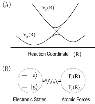
Figure 1: (A) Schematic atomic potentials in terms of adiabatic (solid) and diabatic (dashed) representations for the electronic ground and first excited states along the reaction coordinate. (B) Measurement analogy by regarding the atomic motion as quantum measurement which continuously probes the electronic states by, for instance, the distinct forces experienced.

Among the trajectory-based surface hopping methods, the most popular one is Tully’s fewest switches surface hopping (FSSH) approach Tul90 , together with its variations Bar11 . In this approach, nonadiabatic dynamics is treated by allowing hops from one PES to another, with the hopping probability determined by the weight change of the respective electronic states that are in a quantum superposition. From observation that the classical atomic motion must decohere the electronic subsystem (from quantum superposition), considerable efforts were pushed towards accounting for the associated decoherence effect Sch96 ; Tha98 ; Pre99 ; Sch05 ; Zhu05 ; Gra07 ; Sub11 .

One may notice that the FSSH treatment has an obvious flaw from basic physical point of view. By an analogy with quantum measurement or the popular Schrödinger’s Cat paradox, as illustrated in Fig. 1(B), the FSSH scheme simply indicates that, while having found the Cat definitely “alive” or “dead”, one is still treating the radioactive decay in “quantum superposition”. In addition, it was also noticed that the FSSH scheme involves a man-made hopping algorithm to generate the stochastic surface-switching events Bar11 ; Pre99 ; Sch05 . In this work, by explicitly identifying the role of the atomic motion as a quantum measurement to the electronic subsystem, we propose a novel quantum trajectory mean field (QTMF) approach to nonadiabatic MD simulations. The protocol is developed from an insight that the involved quantum weak measurement actually serves as an interface between the quantum and classical parts of the MQC strategy. Our scheme also naturally unifies the Ehrenfest-type mean field theory and the trajectory surface-hopping method. As illustrated by excellent agreement with the exact results on the three representative models discussed by Tully Tul90 , the QTMF approach can eliminate all the unsatisfactory features of the FSSH method.

II Formulation

Let us start with the electronic Hamiltonian

$$H_{el}(r;\textbf{R})=-\sum_{j}\frac{\hbar^{2}}{2m_{j}}\nabla_{j}^{2}+v(r;\textbf{R}).$$ (1)

The potential $v(r;\textbf{R})$, which includes the nuclear potential, depends on electronic coordinates operator $r\equiv\{r_{j}\}$ and also atomic configuration, $\textbf{R}\equiv\{R_{\alpha}(t)\}$, that is assumed a set of classical dynamics variables. Expand the electronic wavefunction with an orthogonal basis set functions, $\Psi(r,t;\textbf{R})=\sum_{j}c_{j}(t)\phi_{j}(r;\textbf{R})$. In particular one often exploits the Born-Oppenheimer (BO) adiabatic wavefunctions. These are the instantaneous eigenstates of $H_{el}(r;\textbf{R})$, satisfying $H_{el}(r;\textbf{R})\phi_{j}(r;\textbf{R})=\varepsilon_{j}(\textbf{R})\phi_{j}(r;\textbf{R})$, the standard output of quantum chemistry computation. Each BO energy serves as the BO potential energy surface (PES), $\varepsilon_{j}(\textbf{R})\equiv{V}_{j}(\textbf{R})$, for nuclear motion.

Without loss of generality, we proceed with the BO representation hereafter. The Schrödinger equation for the coherent electronic evolution reads

$$\dot{c}_{j}=-\frac{i}{\hbar}V_{j}(\textbf{R})\,c_{j}-\sum_{k}\dot{\textbf{R}}\cdot\textbf{d}_{jk}(\textbf{R})\,c_{k},$$ (2)

with the nonadiabatic coupling characterized by

$$\textbf{d}_{jk}(\textbf{R})=\langle\phi_{j}(r,\textbf{R})|\nabla_{\textbf{R}}|\phi_{k}(r,\textbf{R})\rangle\,.$$ (3)

Treating atomic motion with classical trajectories on individual PESs, $\{V_{j}(\textbf{R})\}$, the highly celebrated FSSH method Tul90 goes by a Monte-Carlo algorithm as follows. It uses Eq. (2) for the hopping probability from a given ${V}_{j}(\textbf{R})$ to another. That is $p_{j}(t)=\left[|c_{j}(t)|^{2}-|c_{j}(t+\Delta t)|^{2}\right]/|c_{j}(t)|^{2}$, the normalized population change in the BO electronic state $|\phi_{j}(\textbf{R})\rangle$. However, this algorithm is of problematic basis. It completely neglects the influence of classical trajectories back onto the electronic state evolution.

Atomic motion that experiences a series of single PESs should collapse the electronic state from a quantum superposition, given by Eq. (2), onto the corresponding single BO basis state, due to the entanglement-type correlation between the two subsystems. In other words, atomic motion is continuously extracting information on the electronic state, via the correlation between the PES and BO basis state. For instance, the force experienced by atomic motion plays essentially the same role as the meter’s output in quantum measurement process. Based on this insight, we propose to apply the well-established quantum trajectory equation, in replacement of Eq. (2), to account for the backaction effect of the atomic “meter” on the electronic subsystem WM10 :

$$\dot{\rho}(t) =-\frac{i}{\hbar}\left[{H}_{el}(\textbf{R}),\rho(t)\right]+\sum_{j\neq k}\Gamma_{jk}{\cal D}\left[M_{jk}(\textbf{R})\right]\rho(t)$$

$$\quad+\sum_{j\neq k}\sqrt{\gamma_{{\rm F},jk}+\gamma^{\prime}_{jk}}{\cal H}\left[M_{jk}(\textbf{R})\right]\rho(t)\xi_{jk}(t).$$ (4)

In this equation, $\rho$ denotes the reduced density matrix of electronic state, with diagonal elements for BO-state population probabilities, and off-diagonal ones for their coherence. The first term in Eq. (II) describes the same coherent dynamics of Eq. (2), corresponding to the Ehrenfest mean-field approach. The second term accounts for the decoherence effect owing to ensemble average of the nuclear degrees of freedom, with an overall rate $\Gamma$. The third term, significantly, reflects the backaction effect of the atomic motion in each single trajectory realization, with a rate $\gamma_{\rm F}$ for force-mediated information gain and $\gamma^{\prime}$ for information gain by other means, e.g., the nuclear coordinate (atomic configuration) and velocity (atomic kinetic energy). Here we omitted the PES indices of the rates for brevity and for a general description. In the following Sec. II (A) and (B) we will explain how these rates can be implemented in MQC-MD simulation. Before that, we describe in more detail the decoherence and measurement backaction terms.

The second decoherence term in Eq. (II) is associated with a Lindblad superoperator ${\cal D}[M_{jk}]\rho=M_{jk}\rho M_{jk}^{\dagger}-\frac{1}{2}\{M_{jk}^{\dagger}M_{jk},\rho\}$, where $M_{jk}(\textbf{R})=|\phi_{j}(\textbf{R})\rangle\langle\phi_{j}(\textbf{R})|-|\phi_{k}(\textbf{R})\rangle\langle\phi_{k}(\textbf{R})|$ indicates a dephasing between states $\phi_{j}(\textbf{R})$ and $\phi_{k}(\textbf{R})$. The last backaction term, explicitly, is described in terms of an superoperator as ${\cal H}[M_{jk}]\rho=M_{jk}\rho+\rho M_{jk}^{\dagger}-\langle M_{jk}+M_{jk}^{\dagger}\rangle\rho$, where $\langle M_{jk}+M_{jk}^{\dagger}\rangle\equiv{\rm Tr}[(M_{jk}+M_{jk}^{\dagger})\rho]$. Involved in Eq. (II) for this back-action effect are also the quantum jump (from the Copenhagen postulate) related stochastic noises, $\{\xi_{jk}(t)\}$, which satisfy the ensemble average property of ${\rm E}[\xi_{jk}(t)\xi_{j^{\prime}k^{\prime}}(t^{\prime})]=\delta_{jk,j^{\prime}k^{\prime}}\delta(t-t^{\prime})$. From the quantum trajectory theory WM10 , the last term in Eq. (II) has a role of collapsing the electronic state from a quantum superposition onto a single BO basis state. Therefore, now, the issue on “devising” hopping algorithms that are not contained in Eq. (2) does no longer exist anymore.

II.1 Information Gain Rates

In the MQC-MD approach, the nuclear part is treated classically. As a consequence, just like Tully pointed out in his pioneering work Tul90 , the classical force experienced by the atomic motion in the no-transition adiabatic area should come from a single PES. This indicates that, from a measurement perspective, the classical force plays a role of measurement output. Below we analyze this force-mediated information gain rate ($\gamma_{\rm F}$).

We know that the emergence of classicality from a closed quantum system is a fundamental puzzle in quantum mechanics. In essence, this transition is accompanied by quantum jumps. This implies that the classical force has certain stochastic fluctuations. Since the atomic motion is much slower than its electronic counterpart, it would be reasonable to use a coarse-graining force to evolve the Newton equation. Let us denote the coarse-grained fluctuating component by $\tilde{F}_{j}(t)$, which is an average over a characteristic time “$\tau_{c}$” around $t$ as follows:

$$\tilde{F}_{j}(t)=\frac{1}{\sqrt{\tau_{c}}}\int^{t+\tau_{c}/2}_{t-\tau_{c}/2}{\rm d}t^{\prime}\xi_{j}(t^{\prime})\bar{F}_{j}.$$ (5)

$\bar{F}_{j}$ is the BO force associated with the $j_{\rm th}$ PES at $\textbf{R}(t)$. Notice also that $\xi_{j}{\rm d}t={\rm d}W_{j}$, the Wiener increment, has a magnitude order and dimension of $\sqrt{{\rm d}t}$ WM10 . As a result, the coarse-grained $\tilde{F}_{j}(t)$ is no longer $\delta$-function correlated, but has a correlation function of

$${\rm E}[\tilde{F}_{j}(t)\tilde{F}_{j}(0)]=\left\{\begin{array}[]{cc}(\bar{F}_{j})^{2}(\tau_{c}-t)/\tau_{c},&~{}~{}0<t<\tau_{c}\\ (\bar{F}_{j})^{2}(\tau_{c}+t)/\tau_{c},&~{}-\tau_{c}<t<0\end{array}\right.$$ (6)

where ${\rm E}[\cdots]$ denotes an ensemble average over the stochastic realization $\xi_{j}$, which satisfies ${\rm E}[\xi_{j}(t)\xi_{j}(t^{\prime})]=\delta(t-t^{\prime})$. Accordingly, the zero-frequency spectrum of the force-force correlation function reads

$$S_{j}=\int^{\infty}_{-\infty}{\rm d}t~{}{\rm E}[\tilde{F}_{j}(t)\tilde{F}_{j}(0)]=(\bar{F}_{j})^{2}\tau_{c}.$$ (7)

Now we return to the original (stochastic) force of the $j_{\rm th}$ PES, ${\cal F}_{j}(t)=\bar{F}_{j}(t)+\sqrt{S_{j}}\xi_{j}(t)$. The total average force $F_{j}$, given by averaging ${\cal F}_{j}$ over time interval $(t,t+\tau_{m})$, is a stochastic variable satisfying a Gaussian distribution $P(F_{j})=(2\pi D_{j})^{-1/2}\exp[-(F_{j}-\bar{F}_{j})^{2}/2D_{j}]$, with the variance given by $D_{j}=S_{j}/\tau_{m}$. Following the theory for realistic quantum measurements Mtime , the state distinguishable criterion

$$\sqrt{D_{j}}+\sqrt{D_{k}}\leq|\bar{F}_{j}-\bar{F}_{k}|,$$ (8)

allows us to extract the measurement time ($t_{m}$) which is minimally required to identify the state being ${\left|\phi_{j}\right\rangle}$ or ${\left|\phi_{k}\right\rangle}$. Obviously, $t_{m}$ is given by $\tau_{m}$ from Eq. (8) in the case of equality. Then, the information gain rate $\gamma_{{\rm F},jk}$ in Eq. (II) coincides with $1/t_{m}$, taking a compact form as,

$$\gamma_{{\rm F},jk}=\frac{(\bar{F}_{j}-\bar{F}_{k})^{2}}{(|\bar{F}_{j}|+|\bar{F}_{k}|)^{2}}\frac{1}{\tau_{c}}\,.$$ (9)

As inferred from the coarse-grained force, the characteristic time $\tau_{c}$ physically scales atomic motion that is typically of picosecond. With respect to the femtosecond timescale of the electronic part, in practice we adopt $1/\tau_{c}\simeq 10^{-3}$ in (reduced) units of the electronic energies. Favorably, the information gain rate given by Eq. (9) is of configuration (R) dependence, but it does not need any microscopic information of the nuclear (quantum) wavepackets. It allows thus for a convenient implementation even for simulation on complex molecular systems.

Except for the force-mediated information gain discussed above, there exit also other channels of information gain, which are formally accounted for by $\gamma^{\prime}$ in Eq. (II). The channels include the nuclear coordinate R and velocity $\dot{\textbf{R}}$ in the MQC-MD simulation. For instance, if we performed a microscopic full quantum treatment, the nuclear wavepacket would have distinct spatial extension along different PES. With this “knowledge” in priori, one can infer certain information for the electronic state from the classical “output” R. Another information channel is the nuclear kinetic energy (associated with $\dot{\textbf{R}}$). For an initial state with specific energy, the distinct kinetic energies on different PESs in MQC-MD simulation exposure also some information of the electronic state. Unfortunately, to our knowledge, the information gain rates through these channels have not yet well developed so far. However, fortunately, as we will elaborate further in next subsection, the specific form of these rates are not important for us to get the correct results.

II.2 More Remarks on Eqs. (II) and (9)

Generally speaking, a desirable MQC-MD approach should satisfy two requirements. One is that the equation for the electronic subsystem should satisfy the ensemble average property, corresponding to averaging the nuclear degrees of freedom from the exact dynamics of the full electronic-plus-nuclear system. Another is that the equation should allow for performing reasonable classical MD simulation (with correct “force” and “kinetic energy”) on the nuclear subsystem. Our protocol is to combine Eq. (II) with a classical MD simulation to fulfill these two requirements. That is, the second term of Eq. (II) satisfies the first requirement, and the last term satisfies the second one.

In Eq. (II), we distinguished the information-gain rates $\gamma_{\rm F}$ and $\gamma^{\prime}$ from the overall decoherence rate $\Gamma$. Formally, we may express $\Gamma=\gamma_{\rm F}+\gamma^{\prime}+\tilde{\gamma}$. As discussed above in Sec. II (A), $\gamma_{\rm F}$ and $\gamma^{\prime}$ are, respectively, the information gain rates mediated by force and other channels (e.g., R and $\dot{\textbf{R}}$). Therefore, $\tilde{\gamma}$ represents the decoherence rate not unraveled (the rate of information loss). For practical applications, we propose the following strategies to implement these rates:

1. In the nonadiabatic crossing region, use the rate $\gamma_{\rm F}$ given by Eq. (9) to approximate the total information gain and decoherence rates. This approximation is from an insight that, in the conical intersection area, the total decoherence rate should be quite weak, otherwise the result will be strongly distorted from the correct one (the Ehrenfest mean-field approach is a support to this viewpoint). We believe that our coarse-graining argument for obtaining Eq. (9) gives a reasonable order of magnitude for this rate.

2. Apart from the crossing area, add a nonzero $\gamma^{\prime}$ into Eq. (II), by using a simple phenomenological parameter with similar/stronger magnitude order of $1/\tau_{c}$, or by certain more sophisticated manner Sch05 ; Sub11 ; Nitz93 . We may remark that this different implementation of $\gamma^{\prime}$ is anticipated to result in slight difference only in the “narrow” region between the nonadiabatic crossing and the no-transition adiabatic areas. It will affect neither the molecular dynamics in the broad adiabatic region, nor the ensemble statistical properties. For the overall decoherence rate $\Gamma$, one can set either $\Gamma=\gamma_{\rm F}+\gamma^{\prime}$, or $\Gamma=\gamma_{\rm F}+\gamma^{\prime}+\tilde{\gamma}$ by including a more information-loss rate. However, $\tilde{\gamma}$ will have no effect, since $\gamma_{\rm F}$ and $\gamma^{\prime}$ will collapse the system in the adiabatic area onto a single PES in each trajectory realization, implying a mixed state after ensemble average. The role of $\tilde{\gamma}$ is simply to facilitate the formation of an ensemble-averaged mixed state.

Finally, we mention a special case that may remind our attention. For parallel PESs, the “force output” reveals no information of the electronic state, thus giving a vanished measurement rate. This is in consistence with the result of Eq. (9). In this case, the rate $\gamma^{\prime}$ from other informational channels will collapse the system onto a single PES in the adiabatic area. Whether or not collapsing the system onto a single PES in this case will have no effect on the force, but it does affect the kinetic energy (nuclear velocity) that should be of importance in the MD simulation for real molecular systems.

II.3 Issue of Energy Conservation

In the MQC-MD approach, the atomic motion defines a time-dependent electronic Hamiltonian, which does not conserve the electronic energy. In turn, the electronic energy defines a potential to guide the classical motion of atoms. The sum of the kinetic and potential energies, $E=K+{\rm Tr}[H_{el}(\textbf{R})\rho(\textbf{R})]\equiv K+V(\textbf{R})$, is conserved, simply as the situation in the Ehrenfest mean-field approach.

However, Eq. (II) is stochastic. This would lead to a stochastic potential energy $V(\textbf{R})$. The non-analytic $V(\textbf{R})$ makes the force not perfectly defined in mathematics, causing thus some errors in determining the nuclear velocity. This would violate slightly the total energy conservation. Noticeably, in the present QTMF approach, this violation is quite weak (particularly if a coarse graining procedure is involved), unlike the drastic violation in the FSSH scheme where an energy calibration must be performed after each hopping event. For practice of the QTMF approach, we propose the following scheme to address this issue:

1. Define the whole simulation region with the criterion $V(\textbf{R})\leq E_{0}$, where $E_{0}$ is the initial energy of the whole system. Of course, this renders also that $V_{j}(\textbf{R})\leq E_{0}$ once the system is fully collapsed onto the $j_{\rm th}$-PES.

2. If $V(\textbf{R}_{1})=E_{0}$ occurs at $\textbf{R}_{1}$, reset the system to its proximity point $\textbf{R}_{2}$, given by $V_{M}(\textbf{R}_{2})=E_{0}$. Here, $V_{M}$ is the renormalized Ehrenfest mean-field potential energy and determined as follows: at $\textbf{R}_{2}$, keep the electronic wavefunction unchanged as the one at $\textbf{R}_{1}$; subtract the lowest PES component and re-normalize the wavefunction; then use the renormalized wavefunction to calculate the Ehrenfest $V_{M}(\textbf{R}_{2})$.

3. Restart the MD evolution from the determined proximity point $\textbf{R}_{2}$, with the original superposition of BO PESs at $\textbf{R}_{1}$ but a newly assigned atomic kinetic energy of $E_{0}-{V}(\textbf{R}_{2})$ and the momentum direction opposite to that at $\textbf{R}_{1}$.

4. After passing through the nonadiabatic crossing area, check the total energy of the collapsed state (onto a single PES) and make it be $E_{0}$ via proper modification to the kinetic energy.

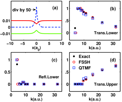
Figure 2: Single-avoided crossing model. In (a) we depict the adiabatic potential sufaces (solid) and the nonadiabatic coupling strength (dashed, given by Eq. (3)). Displayed in (b), (c) and (d) are, respectively, the probabilities of transmission to the upper surface, reflection to the lower surface, and transmission to the upper surface. For comparison, we put together the results of our QTMF and Tully’s FSSH approaches against with the exact one of quantum dynamics simulation.

III Illustrative Examples

In this section we present our QTMF results versus the exact and FSSH counterparts, on the well-known set of Tully test systems Tul90 , each of them being a one-dimensional two-surface model, with an atomic mass of $M=2000$ a.u. (all parameters below are in atomic unit). The scheme for exact quantum dynamics simulation was clearly described in Ref. Tul90 . In the present work, we simply extract the results from Ref. Tul90 for comparison. In our simulation, we assume an incident energy $E_{0}=k^{2}/(2M)$ to initiate the system evolution. And, as discussed earlier, we adopt $1/\tau_{c}=10^{-3}$. In the nonadiabatic coupling area, we approximate the entire decoherence and information rates by $\gamma_{\rm F}$ through Eq. (9). In the adiabatic (no-transition) area, we add $\gamma^{\prime}=10^{-2}$ to account for the backaction effect of other informational channels, and set $\Gamma=\gamma_{\rm F}+\gamma^{\prime}$. As explained in Sec. II (A) and (B), the choice of $\gamma^{\prime}$ in the adiabatic area can be rather arbitrary, having almost no influence on the results. For each model, we run $2000$ stochastic trajectories and accordingly determine the population probabilities of the final “products”. Also, each trajectory begins with the classical particle (atom) on the lower energy surface at $x=-10$, with an incident momentum to the right, and ends at $|x|=15$.

Model-I: Single-Avoided Crossing – The diabatic potential matrix elements for this model are

$$\begin{split}&V_{11}(x)=-V_{22}(x)=\text{sign}(x)\cdot A[1-\exp(-Bx)],\\ &V_{12}(x)=V_{21}(x)=C\exp(-Dx^{2}).\end{split}$$ (10)

Set $A=0.01$, $B=1.6$, $C=0.005$, and $D=1$. The adiabatic potential surfaces of this model are plotted in Fig. 2(a), while the results are shown in Fig. 2(b)-(d). Desirably, both our QTMF and the FSSH schemes work very well for this model, being almost in an overall agreement with the exact results. We only make two remarks on the extremely quantum regime. (i) The steep step-function behavior at $k\sim 5$ is an indicator for the failure of almost all semiclassical MD methods, i.e., failing to predict tunneling through the barrier on the lower surface at very low momentum. Physically, in our case this is caused by setting the semiclassical rule of energy-conservation when propagating the state. Giving up this restriction at $k\sim 5$, we can actually recover the exact result. (ii) Another interesting quantum regime is $k\sim 8$ ($7.7<k<8.9$), which is above the threshold for transmission. Satisfactorily, both QTMF and FSSH captured the essential physics here, e.g., predicting the small amount of particle reflections. This is somehow a challenging test for any semiclassical approaches.

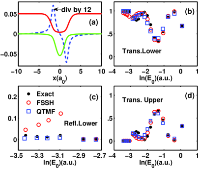
Figure 3: Dual-avoided crossing model. Shown in (a) is the adiabatic potential surfaces (solid) together with the nonadiabatic coupling strength (dashed), while in (b), (c) and (d) are the transmission and reflection probabilities as stated in Fig. 2.

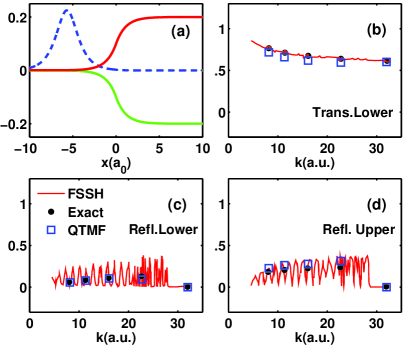
Figure 4: Extended coupling model. Shown in (a) is the adiabatic potential surfaces (solid) together with the nonadiabatic coupling strength (dashed), while in (b), (c) and (d) are the transmission and reflection probabilities as stated in Fig. 2.

Model-II: Dual-Avoided Crossing – This is a more challenging model and contains two avoided crossings. The key feature of this model is the Stueckelberg oscillations, owing to quantum interference between the successive nonadiabatic quantum transitions. The diabatic potentials for this model are given by

$$\begin{split}&V_{11}(x)=0,\ \ \ V_{22}(x)=-A\exp(-Bx^{2})+E,\\ &V_{12}(x)=V_{21}(x)=C\exp(-Dx^{2}),\end{split}$$ (11)

where $A=0.10$, $B=0.28$, $C=0.015$, $D=0.06$, and $E=0.05$. The adiabatic potentials of this model and results comparison are shown in Fig. 3. At high incident energies, both the FSSH and QTMF can give correct results in good agreement with the exact ones, all exhibiting the expected Stueckelberg oscillations. However, at low energies, the FSSH method fails to predict both the transmission and reflection probabilities on the lower surface, see Fig. 3 (b) and (d) in the low energy regime. In particular, the FSSH algorithm overestimates the amount of reflection by an order of magnitude (roughly a factor of 10). This overestimation is owing to the artificial hopping algorithm, which results in too many upward transitions. In sharp contrast, our QTMF approach can physically rule out this drawback.

Model-III: Extended Coupling – This is the most challenging model for classical mechanics based approach to address, since it involves an extended region of strong nonadiabatic coupling. The diabatic potentials are

$$\begin{split}&V_{11}=-V_{22}=A,\\ &V_{12}=V_{21}=\begin{cases}B\exp(Cx);&x<0,\\ B[2-\exp(-Cx)];&x>0.\end{cases}\end{split}$$ (12)

The parameters are $A=6\times 10^{-4}$, $B=0.1$ and $C=0.9$. The adiabatic potentials and comparative results are shown in Fig. 3. We see that, unfortunately, the FSSH algorithm completely fails for the reflection probabilities, to either the upper or lower surface. This failure clearly indicates that the FSSH algorithm breaks down in strong quantum transition region. Again, in sharp contrast, our QTMF approach gives satisfactory results even for this very demanding model.

IV Summary

To summarize, we have proposed a quantum trajectory mean field (QTMF) approach to the powerful mixed-quantum-classical molecular dynamics simulation with surface hopping. Simulations on three nontrivial models are quantitatively satisfactory. While Eq. (9) offers a compact position-dependent measurement rate on atomic motion timescale ($\tau_{c}$), the present study reveals also an important observation: results are rather insensitive to the choice of decoherence rate, as long as it is weak ($\sim 1/\tau_{c}$) in the nonadiabatic crossing area. Unraveling any decoherence rate in the no-transition adiabatic area can stochastically collapse the system onto a single potential surface, and gives about the same satisfactory statistical results.

In this context we would like to remark that quantum superposition is rooted in the exact quantum dynamics simulation, but involving not at all the concept of classical atomic trajectory. In Tully’s fewest switches algorithm, while the evolution of electronic state is not consistent with the successive complete surface hopping, it keeps the essential feature of quantum superposition. It is merely this reason, in our opinion, that makes the most celebrated FSSH approach be often comparable to the exact results from full quantum dynamics simulation.

Compared with the FSSH approach, the QTMF scheme is founded on a more physical and simpler treatment. For the electronic part, the replacement of the Schrödinger equation with a master equation will increase only negligible amount of computational complexity, since the involved BO states are very few (for instance, only two in most real molecular simulations). On the other hand, the QTMF scheme avoids the hopping algorithm and simplifies the procedures of calibrating the total energy. This will speed the simulation. As a conservative estimate, the time cost of the QTMF scheme is comparable to or less than the FSSH approach (and its many variations). With this computational efficiency together with the satisfactory accuracy, and most importantly its physical foundation, the proposed QTMF scheme is anticipated to be a powerful tool in real MD simulations.

Acknowledgments— This work was supported by the Major State Basic Research Project of China (Nos. 2011CB808502 & 2012CB932704) and the NNSF of China (Nos. 101202101 & 10874176 & 21033008).

References

- (1) J. C. Tully, Faraday Discuss 110, 407 C419 (1998).
- (2) For a recent review, see M. Barbatti, WIREs Comput. Mol. Sci. 1, 620 (2011).
- (3) R. B. Gerber, V. Buch, and M. A. Ratner, J. Chem. Phys. 77, 3022 (1982).
- (4) D. A. Micha, J. Chem. Phys. 78, 7138 (1983).
- (5) X. Li, J. C. Tully, H. B. Schlegel, and M. J. Frisch, J. Chem. Phys. 123, 084106 (2005).
- (6) J. C. Tully, P. K. Preston, J. Chem. Phys 55, 562 (1971).
- (7) W. H. Miller and T. F. George, J. Chem. Phys. 56, 5637 (1972).
- (8) P. J. Kuntz, J. Kendrick, and W. N. Whitton, Chem. Phys. 38, 147(1979).
- (9) N. C. Blais and D. G. Truhlar, J. Chem. Phys. 79, 1334 (1983).
- (10) D. P. Ali and W. H. Miller, J. Chem. Phys. 78, 6640 (1983).
- (11) J. C. Tully, J. Chem. Phys. 93, 1061 (1990).
- (12) P. J. Kuntz, J. Chem. Phys. 95, 141 (1991).
- (13) F. Webster, E. T. Wang, P. J. Rossky, and R. A. Friesner, J. Chem. Phys. 100, 4835 (1994).
- (14) O. V. Prezhdo and P. J. Rossky, J. Chem. Phys. 107, 825 (1997).
- (15) C. Zhu, A. W. Jasper, and D. G. Truhlar, J. Chem. Phys. 120, 5543 (2004).
- (16) B. J. Schwartz, E. R. Bittner, O. V. Prezhdo, and P. J. Rossky, J. Chem. Phys. 104, 5942 (1996).
- (17) M. Thachuk, M. Y. Ivanov, and D. M. Wardlaw, J. Chem. Phys. 109, 5747 (1998).
- (18) O. V. Prezhdo, J. Chem. Phys. 111, 8366 (1999).
- (19) M. J. Bedard-Hearn, R. E. Larsen, and B. J. Schwartz, J. Chem. Phys. 123, 234106 (2005).
- (20) C. Zhu, A. W. Jasper, and D. G. Truhlar, J. Chem. Theor. Comput. 1, 527 (2005).
- (21) G. Granucci, M. Persico, J. Chem. Phys. 126, 134114 (2007).
- (22) J. E. Subotnik and N. Shenvi, J. Chem. Phys. 134, 024105 (2011).
- (23) H. M. Wiseman and G. J. Milburn, Quantum Measurement and Control (Cambridge University Press, 2010).
- (24) I. L. Aleiner, N. S. Wingreen, and Y. Meir, Phys. Rev. Lett. 79, 3740 (1997); Y. Makhlin, G. Schön, and A. Shnirman, Rev. Mod. Phys. 73, 357 (2001); A. A. Clerk, M. H. Devoret, S. M. Girvin, F. Marquardt, and R. J. Schoelkopf, Rev. Mod. Phys. 82, 1155 (2010).
- (25) E. Neria and A. Nitzan, J. Chem. Phys. 99, 1109 (1993); Chem. Phys. 183, 351 (1994).