The Matrix Ridge Approximation: Algorithms and Applications

Abstract

We are concerned with an approximation problem for a symmetric positive semidefinite matrix due to motivation from a class of nonlinear machine learning methods. We discuss an approximation approach that we call matrix ridge approximation. In particular, we define the matrix ridge approximation as an incomplete matrix factorization plus a ridge term. Moreover, we present probabilistic interpretations using a normal latent variable model and a Wishart model for this approximation approach. The idea behind the latent variable model in turn leads us to an efficient EM iterative method for handling the matrix ridge approximation problem. Finally, we illustrate the applications of the approximation approach in multivariate data analysis. Empirical studies in spectral clustering and Gaussian process regression show that the matrix ridge approximation with the EM iteration is potentially useful.

Keywords: Positive semidefinite matrices; Matrix ridge approximation; Incomplete matrix factorization; Expectation maximization algorithms; Probabilistic models.

1 Introduction

Symmetric positive semidefinite matrices play an important role in multivariate statistical analysis and machine learning. Especially, the low-rank approximation of a positive semidefinite matrix has been widely applied to multivariate data analysis. In this paper we study the low-rank approximation problem of a positive semidefinite matrix as well as its applications in machine learning. Moreover, we always assume that the positive semidefinite matrix in question is symmetric.

Some machine learning methods require computing the inverse of a positive definite matrix or the spectral decomposition of a positive semidefinite matrix. For example, the kernel PCA (principal component analysis) (Schölkopf and Smola, 2002), classical multidimensional scaling (also called principal coordinate analysis, PCO) (Mardia et al., 1979) and spectral clustering algorithms (Zhang and Jordan, 2008) require solving an eigenvalue problem with linear constraints on an $m{\times}m$ inner-product matrix (Golub, 1973), and Gaussian processes (GPs) (Rasmussen and Williams, 2006) need to invert $m{\times}m$ covariance matrices. Typically, these methods take $O(m^{3})$ operations where $m$ denotes the number of training instances. This scaling is unfavorable for applications in massive datasets.

Several approaches have been also proposed to address this computational challenge, such as randomized techniques (Achlioptas et al., 2001), sparse greedy approximation (Smola and Schölkopf, 2000), and the Nyström method (Williams and Seeger, 2001, Yang et al., 2012). All these approaches are based on sampling techniques. Similar ideas include random Fourier features (Rahimi and Recht, 2008, Quiñonero-Candela et al., 2007, Lázaro-Gredilla et al., 2010, Le et al., 2013) and hashing features (Shi et al., 2009). Specifically, the random feature method avoids inversion of a matrix by solving a linear system of equations instead. Another widely used approach is to employ the incomplete Cholesky decomposition method (Golub and Loan, 1996, Fine et al., 2001). The approach is deterministic. Although these approaches can be efficient, their range of applications might be limited; e.g., these approaches are always infeasible in handling the eigenvalue decomposition problem with linear constraints.

In this paper we present a new deterministic low-rank approximation approach. Roughly speaking, the approach is to approximate a positive semidefinite matrix as an incomplete matrix decomposition plus a ridge term. We refer to such an approximation method as the matrix ridge approximation due to its direct motivation from the ridge regression model (Hoerl and Kennard, 1970). The approximation is built on an optimization problem with linear constraints. This problem can be in turn solved by using the conventional spectral decomposition technique or an efficient iterative method.

Although the idea behind the matrix ridge approximation is simple, our method is attractive. Firstly, it yields an approximation tighter than the incomplete Cholesky decomposition and the incomplete spectral decomposition do. Secondly, it yields an approximate matrix, whose condition number is not higher than that of the original matrix. This can make numerical computations involved more stable. More importantly, it can widen the application range of the low-rank approximation approach. Particularly, we show that our method can be applied to the approximate computation of the inverse and spectral decomposition of a positive (semi)definite matrix. We illustrate the application of the matrix ridge approximation in spectral clustering and Gaussian process regression.

We also discuss two statistical counterparts for the ridge approximation. The first counterpart is in the spirit of probabilistic interpretations of some machine learning methods, including probabilistic PCA (Tipping and Bishop, 1999, Roweis, 1998, Ahn and Oh, 2003), probabilistic nonlinear component analysis (Rosipal and Girolami, 2001), Gaussian process latent variable models (Lawrence, 2004), and factor analysis (Magnus and Neudecker, 1999). In particular, we define a normal latent variable model in which we impose the linear constraints. Based on the latent variable model, we devise an iterative method, i.e., the expectation-maximization (EM) algorithm (Dempster et al., 1977), for solving the matrix ridge approximation problem.

The second counterpart is a Wishart model, which is derived from the normal latent variable model by using the relationship between Wishart distributions and Gaussian distributions (Gupta and Nagar, 2000, Zhang et al., 2006). These two statistical counterparts in turn define probabilistic matrix ridge approximation models. Moreover, we show that the maximum likelihood approach to estimating the parameters of the probabilistic models results in the same solution as that based on the standard spectral decomposition technique.

The remainder of the paper is organized as follows. We first give the notation in Section 2. We present the matrix ridge approximation in Section 3 and illustrate its applications in Section 4. We reformulate the matrix ridge approximation by using a normal latent variable model and a Wishart model in Section 5. Consequently, we develop probabilistic ridge approximation and an EM iterative algorithm. Section 6 conducts the empirical analysis, and Section 7 concludes our work. Note that we put all proofs to the appendices.

2 Notation and Terminology

We let ${\bf I}_{m}$ denote the $m{\times}m$ identity matrix, and ${\bf 1}_{m}$ denote the $m{\times}1$ vector of ones. For a matrix ${\bf Y}$, we denote its rank, Frobenius norm and condition number by $\mathrm{rk}({\bf Y})$, $\|{\bf Y}\|_{F}$ and $\kappa({\bf Y})$, respectively. When ${\bf Y}$ is square, we denote its determinant and trace by $|{\bf Y}|$ and $\mathrm{tr}({\bf Y})$. Additionally, ${\bf A}\otimes{\bf B}$ denotes the Kronecker product of ${\bf A}$ and ${\bf B}$.

For an $s{\times}t$ random matrix ${\bf Z}$, ${\bf Z}\thicksim N_{s,t}({\bf M},{\bf A}{\otimes}{\bf B})$ means that ${\bf Z}=[z_{ij}]$ ($s{\times}t$) follows a matrix-variate normal distribution with mean matrix ${\bf M}=[m_{ij}]$ ($s{\times}t$) and covariance matrix ${\bf A}{\otimes}{\bf B}$, where ${\bf A}$ ($s{\times}s$) and ${\bf B}$ ($t{\times}t$) are symmetric positive definite. Note that a matrix variate normal distribution is defined through a multivariate normal distribution (Gupta and Nagar, 2000). In particular, let $\mathrm{vec}({\bf Z}^{T})=(z_{11},\ldots,z_{1t},z_{21},\ldots,z_{st})^{T}$ ($st{\times}1$) and $\mathrm{vec}({\bf M}^{T})=(m_{11},\ldots,m_{1t},m_{21},\ldots,m_{st})^{T}$ ($st{\times}1$). Then, ${\bf Z}\thicksim N_{s,t}({\bf M},{\bf A}{\otimes}{\bf B})$ if and only if $\mathrm{vec}({\bf Z}^{T})\thicksim N_{st}(\mathrm{vec}({\bf M}^{T}),{\bf A}{\otimes}{\bf B})$. We also use the notation in Gupta and Nagar (2000) for Wishart distributions. That is, for an $m{\times}m$ positive definite random ${\bf Y}$, ${\bf Y}\thicksim W_{m}(r,\mbox{\boldmath$\Sigma$\unboldmath})$ represents that ${\bf Y}$ follows a Wishart distribution with degree of freedom $r$.

Finally, in Table 1 we list some notations that will be used throughout this paper. It is clear that ${\bf H}_{b}{\bf H}_{b}={\bf H}_{b}$ and ${\bf P}{\bf P}={\bf P}$; i.e., they are idempotent. Moreover, we have ${\bf H}_{b}{\bf 1}_{m}={\bf 0}$, ${\bf b}^{T}{\bf H}_{b}={\bf 0}$, ${\bf P}{\bf b}={\bf 0}$ and ${\bf b}^{T}{\bf P}={\bf 0}$. A typical nonzero case for ${\bf b}$ is ${\bf b}=\frac{1}{\sqrt{m}}{\bf 1}_{m}$. This case implies that ${\bf H}_{b}={\bf P}={\bf I}_{m}{-}\frac{1}{m}{\bf 1}_{m}{\bf 1}_{m}^{T}$ and ${\bf A}^{T}{\bf 1}_{m}={\bf 0}$ (that is, the mean of the rows of ${\bf A}$ is zero). In addition, let us keep in mind that ${\bf H}_{b}={\bf P}={\bf I}_{m}$ when ${\bf b}={\bf 0}$ for notational simplicity. In this case we always have ${\bf M}={\bf S}={\bf T}$.

Table 1: Some notations that will be used in this paper.

${\bf b}\in{\mathbb{R}}_{+}^{m}$	a $m$-dimensional nonnegative vector
${\bf M}\in{\mathbb{S}}_{+}^{m{\times}m}$	a positive semidefinite matrix of rank $p$ ($1<p\leq m$)
${\bf H}_{b}={\bf I}_{m}{-}\frac{{\bf 1}_{m}{\bf b}^{T}}{{\bf 1}_{m}^{T}{\bf b}}$ (${\bf b}\neq{\bf 0}$)	centering matrix
${\bf P}={\bf I}_{m}{-}{\bf b}{\bf b}^{T}$	projection matrix
${\bf S}={\bf H}_{b}{\bf M}{\bf H}_{b}^{T}$	positive semidefinite matrix
${\bf T}={\bf P}{\bf M}{\bf P}$	positive semidefinite matrix

3 The Matrix Ridge Approximation

We are given a nonnegative vector ${\bf b}\in{\mathbb{R}}_{+}^{m}$ and a positive semidefinite matrix ${\bf M}\in{\mathbb{S}}_{+}^{m{\times}m}$ of rank $p$ ($1<p\leq m$). The ridge approximation of ${\bf M}$ is defined as

$${\bf M}\thickapprox{\bf A}{\bf A}^{T}+\delta{\bf I}_{m},$$

where $\delta>0$ is called a ridge term, and ${\bf A}\in{\mathbb{R}}^{m{\times}q}$ is a matrix of full column rank $q$ ($<p$) and satisfies ${\bf A}^{T}{\bf b}={\bf 0}$. The idea behind the matrix ridge approximation is simple, and the terminology is motivated by the ridge regression model (Hoerl and Kennard, 1970). Note that when ${\bf b}={\bf 0}$, ${\bf A}^{T}{\bf b}={\bf 0}$ is always true. This implies no constraints. In this paper we consider both the cases with and without the linear constraints. Since ${\bf A}^{T}{\bf b}={\bf 0}$ is equivalent to $c{\bf A}^{T}{\bf b}={\bf 0}$ for any nonzero constant $c$, we assume that ${\bf b}^{T}{\bf b}=1$ whenever ${\bf b}\neq{\bf 0}$ to make the constraint identifiable.

The constraint ${\bf A}^{T}{\bf b}={\bf 0}$ for ${\bf b}\neq{\bf 0}$ is often met in machine learning methods such as the classical multidimensional scaling (Gower and Legendre, 1986), kernel PCA (Schölkopf and Smola, 2002), spectral clustering (Zhang and Jordan, 2008), etc. If ${\bf b}={\bf 0}$ and $\delta=0$, we obtain the incomplete factorization ${\bf M}\thickapprox{\bf A}{\bf A}^{T}$ straightforwardly by using the spectral decomposition of ${\bf M}$ (Magnus and Neudecker, 1999). In this setting, the ridge approximation is also closely related to the incomplete Cholesky factorization (Golub and Loan, 1996). Furthermore, if $q=p$ it is feasible to obtain an exact expression ${\bf M}={\bf A}{\bf A}^{T}$ via the spectral (or Cholesky) decomposition. In this paper we concentrate on the case that $q<p$ and $\delta>0$, so we have a sparse plus low-rank approximation of ${\bf M}$ ($\delta{\bf I}_{m}$ is sparse and ${\bf A}{\bf A}^{T}$ is low-rank).

In order to estimate ${\bf A}$ and $\delta$, we exploit two loss functions which were developed for estimation of covariance matrices (Anderson, 1984). In particular, the first loss function is a least-squares error:

$$F({\bf A},\delta)=\mathrm{tr}\big{[}({\bf S}{-}{\bf A}{\bf A}^{T}{-}\delta{\bf I}_{m})^{2}\big{]}$$

while the second loss is derived from the likelihood function; namely,

$$G({\bf A},\delta)=\log|{\bf A}{\bf A}^{T}+\delta{\bf I}_{m}|+\mathrm{tr}[({\bf A}{\bf A}^{T}+\delta{\bf I}_{m})^{-1}{\bf S}].$$

Theorem 1

Let $\gamma_{1}\geq\cdots\geq\gamma_{q}\geq\cdots\geq\gamma_{m}$ ($\geq 0$) be the eigenvalues of ${\bf S}={\bf H}_{b}{\bf M}{\bf H}_{b}^{T}$, ${\bf V}$ be an arbitrary $q{\times}q$ orthogonal matrix, ${\mbox{\boldmath$\Gamma$\unboldmath}_{q}}$ be a $q{\times}q$ diagonal matrix containing the first $q$ principal (largest) eigenvalues $\gamma_{i}$, and ${{{\bf U}_{q}}}$ be an $n{\times}q$ column-orthonormal matrix in which the $q$ column vectors are the principal eigenvectors corresponding to ${\mbox{\boldmath$\Gamma$\unboldmath}_{q}}$. Assume that $\delta>0$ and that ${\bf A}\in{\mathbb{R}}^{m{\times}q}$ ($q<\min(m,p)$) is of full column rank and satisfies ${\bf A}^{T}{\bf b}={\bf 0}$. If there exists a $j\in\{q{+}1,\ldots,m\}$ such that $\gamma_{q}>\gamma_{j}>0$, then the strict local minimum of $F({\bf A},\delta)$ and of $G({\bf A},\delta)$ with respect to (w.r.t.) $({\bf A},\delta)$ is obtained when

$$\widehat{{\bf A}}={{\bf U}_{q}}({\mbox{\boldmath$\Gamma$\unboldmath}_{q}}-\hat{\delta}{\bf I}_{q})^{1/2}{\bf V}\quad\mbox{and}\quad\hat{\delta}=\frac{1}{m{-}q}\sum_{j=q+1}^{m}\gamma_{j}.$$

Theorem 1 is a direct corollary of Theorem 7 in Appendix B. Theorem 1 also shows that the minimizer $(\widehat{{\bf A}},\hat{\delta})$ of $F({\bf A},\delta)$ is the same to that of $G({\bf A},\delta)$. We consider the case that ${\bf b}=0$. In this case, the condition number of ${\bf M}$ ($={\bf S}$) is $\kappa({\bf M})=\frac{\gamma_{1}}{\gamma_{m}}$. It follows from Theorem 1 that $\kappa(\widehat{{\bf A}}\widehat{{\bf A}}^{T}{+}\hat{\delta}{\bf I}_{m})=\frac{\gamma_{1}}{\frac{1}{m{-}q}\sum_{j=q+1}^{m}\gamma_{j}}\leq\kappa({\bf M})$. This implies that $\widehat{{\bf A}}\widehat{{\bf A}}^{T}{+}\hat{\delta}{\bf I}_{m}$ is well-conditioned more than ${\bf M}$ (Golub and Loan, 1996). In other words, if ${\bf M}$ is well-conditioned, so is $\widehat{{\bf A}}\widehat{{\bf A}}^{T}{+}\hat{\delta}{\bf I}_{m}$.

In addition, it is easily calculated that

$$F(\widehat{{\bf A}},\hat{\delta})=\sum_{i=q{+}1}^{m}\gamma_{i}^{2}-\frac{1}{m{-}q}\Big{(}\sum_{i=q{+}1}^{m}\gamma_{i}\Big{)}^{2}.$$

It is well known that

$$\inf_{\begin{array}[]{c}{\bf B}\in{\mathbb{R}}^{m{\times}m}\\ \mathrm{rk}({\bf B})\leq q\end{array}}\|{\bf S}-{\bf B}\|_{F}^{2}=\inf_{\begin{array}[]{c}{\bf Y}\in{\mathbb{R}}^{m{\times}q}\\ \mathrm{rk}({\bf Y})\leq q\end{array}}\|{\bf S}-{\bf Y}{\bf Y}^{T}\|_{F}^{2}=\sum_{i=q{+}1}^{m}\gamma_{i}^{2}.$$

Thus, when comparing the ridge approximation of ${\bf S}$ with the incomplete Cholesky decomposition of ${\bf S}$, we have

$$\inf_{\begin{array}[]{c}{\bf L}\in{\cal L}\\ \mathrm{rk}({\bf L})=q\end{array}}\|{\bf S}{-}{\bf L}{\bf L}^{T}\|_{F}^{2}\geq\inf_{\begin{array}[]{c}{\bf Y}\in{\mathbb{R}}^{m{\times}q}\\ \mathrm{rk}({\bf Y})=q\end{array}}\|{\bf S}{-}{\bf Y}{\bf Y}^{T}\|_{F}^{2}\geq\inf_{\begin{array}[]{c}\delta\geq 0,{\bf A}\in{\mathbb{R}}^{m{\times}q}\\ \mathrm{rk}({\bf A})=q\end{array}}\|{\bf S}{-}{\bf A}{\bf A}^{T}{-}\delta{\bf I}_{m}\|_{F}^{2},$$

where ${\cal L}=\{{\bf L}\in{\mathbb{R}}^{m{\times}q}:{\bf L}\mbox{ is lower triangular}\}$. This shows that the ridge approximation yields a tighter approximation of ${\bf S}$ than both the incomplete Cholesky decomposition and the incomplete spectral decomposition do.

As we mentioned, $G({\bf A},\delta)$ is associated with a likelihood function. In Section 5.1 we will show that $G$ is derived from a normal latent variable model. Thus, the solution in Theorem 1 is in fact the conventional maximum likelihood (ML) estimate. Furthermore, the ML estimation method is based on the direct spectral decomposition of the $m{\times}m$ matrix ${\bf M}$ or ${\bf S}$, which takes $O(m^{3})$ operations. Thus, the method is inefficient when $m$ is very large. Based on the idea behind the latent variable model, we develop an iterative method for solving the matrix ridge approximation.

In particular, given the $t$th estimates ${\bf A}_{(t)}$ and $\delta_{(t)}$ of ${\bf A}$ and $\delta$, the next estimates of ${\bf A}$ and $\delta$ in our iterative method are given as:

$${\bf A}_{(t{+}1)} = {\bf S}{\bf A}_{(t)}\big{(}\delta_{(t)}{\bf I}_{q}+\mbox{\boldmath$\Sigma$\unboldmath}_{(t)}^{-1}{\bf A}_{(t)}^{T}{\bf S}{\bf A}_{(t)}\big{)}^{-1},$$ (1)

$$\delta_{(t{+}1)} = \frac{1}{m}\Big{[}\mathrm{tr}({\bf S})-\mathrm{tr}\big{(}{\bf A}_{(t{+}1)}\mbox{\boldmath$\Sigma$\unboldmath}_{(t)}^{-1}{\bf A}_{(t)}^{T}{\bf S}\big{)}\Big{]},$$ (2)

where $\mbox{\boldmath$\Sigma$\unboldmath}_{(t)}=\delta_{(t)}{\bf I}_{q}+{\bf A}_{(t)}^{T}{\bf A}_{(t)}$. Derivation of the algorithm is given in Section 5.1 and Appendix E. This procedure involves multiplication of $m{\times}m$ matrices by $m{\times}q$ matrices and inversion of $q{\times}q$ matrices. Inverting a $q{\times}q$ matrix takes $O(q^{3})$ operations, and multiplying an $m{\times}m$ matrix by an $m{\times}q$ matrix runs in $m^{2}q$ flops. Thus, this method takes time $O(Tm^{2}q)$, where $T$ is the maximum iterative number. The method is efficient because $T$ is usually far smaller than $m$ (even smaller than $\sqrt{m}$), especially when $m$ is vary large. In the following experiment, we will see that in most cases the EM iterations get convergence after about 20 steps. Moreover, the matrix multiplication can be easily implemented in parallel. Additionally, the EM method does not necessarily load whole $m{\times}m$ matrix ${\bf S}$ during the iterations, which can significantly reduce the storage space.

Given an initial matrix ${\bf A}_{(0)}$ such that $\mathrm{range}({\bf A}_{(0)})\subseteq\mathrm{range}({\bf S})$ where $\mathrm{range}({\bf Z})$ represents the space spanned by the columns of ${\bf Z}$, we have the following lemma.

Lemma 2

Assume that the matrices $\{{\bf A}_{(t)}\}$ are generated by (1) and (2). If $\mathrm{range}({\bf A}_{(0)})\subseteq\mathrm{range}({\bf S})$ and $\mathrm{rk}({\bf A}_{(0)})=q$, then for all $t>1$, the ${\bf A}_{(t)}$ are of full column rank.

In Section 5.1 we will show that the iterative method given in (1) and (2) is a standard EM iterative procedure (Dempster et al., 1977). Consequently, its convergence has been well established (Wu, 1983). The following theorem proves that the constraints ${\bf A}_{(t)}^{T}{\bf b}={\bf 0}$ always hold during the iteration procedure and the EM estimates converge to the corresponding ML estimates. In other words, the EM iteration converges to the strict local minimizer.

Theorem 3

Given initial values $\delta_{(0)}$ and ${\bf A}_{(0)}$ subject to $\delta_{(0)}>0$ and ${\bf A}_{(0)}^{T}{\bf b}={\bf 0}$, the values of ${\bf A}_{(t)}$ and $\delta_{(t)}$ calculated via (1) and (2) always satisfy ${\bf A}_{(t)}^{T}{\bf b}={\bf 0}$ and $\delta_{(t)}>0$. Moreover, the EM estimates of ${\bf A}$ and $\delta$ converge to the conventional ML solutions given in Theorem 1.

The EM algorithm provides an efficient iterative method for computing the matrix ridge approximation. This iterative method is related to the power method and the Lanczos method (Golub and Loan, 1996), which typically serve for solving matrix eigenvector problems numerically. Specifically, this EM algorithm is similar to the QR orthogonal iteration, which is a straightforward generalization of the power method to find a higher-dimensional invariant subspace (Golub and Loan, 1996).

Intuitively, it seems interesting that we consider a two-step procedure to solve the matrix ridge approximation as follows. Specifically, we first apply the QR orthogonal iteration to obtain an $m{\times}q$ column-orthonormal matrix ${\bf Q}$ and set $\widehat{{\bf A}}={\bf Q}({\bf Q}^{T}{\bf S}{\bf Q})^{1/2}$. We then calculate $\hat{\delta}=\frac{\mathrm{tr}({\bf S})-\mathrm{tr}({\bf Q}^{T}{\bf S}{\bf Q})}{m}$ based on the minimization of $\mathrm{tr}(({\bf S}-\widehat{{\bf A}}\widehat{{\bf A}}^{T}-\delta{\bf I}_{m})^{2})$ w.r.t. $\delta$. Assume that ${\bf Q}^{T}{\bf S}{\bf Q}=\mbox{\boldmath$\Gamma$\unboldmath}_{q}$. Then $\hat{\delta}=\frac{\sum_{i=q{+}1}^{m}\gamma_{i}}{m}$. It is directly computed that

$$\mathrm{tr}(({\bf S}-\widehat{{\bf A}}\widehat{{\bf A}}^{T}-\hat{\delta}{\bf I}_{m})^{2})=\sum_{i=q{+}1}\gamma_{i}^{2}-\frac{1}{m}\Big{(}\sum_{i=q{+}1}\gamma_{i}\Big{)}^{2}>\sum_{i=q{+}1}\gamma_{i}^{2}-\frac{1}{m-q}\Big{(}\sum_{i=q{+}1}\gamma_{i}\Big{)}^{2}.$$

This implies that the two-step procedure can not find the optimum solution of the matrix ridge approximation problem. Moreover, we have $\kappa(\widehat{{\bf A}}\widehat{{\bf A}}^{T}+\hat{\delta}{\bf I}_{m})=1+\frac{m\gamma_{1}}{\sum_{i=q{+}1}^{m}\gamma_{i}}$. Compared with our method, this two-step method results in the approximation with higher condition number. Moreover, the method can not keep the well-conditionedness of the original matrix (if it is well-conditioned). We will conduct simulation on a toy data in Section 6.1, which shows that the two-step method fails to solve the matrix ridge approximation problem.

It is worth noting that the nonnegativity on ${\bf b}$ is not necessary in our derivation for the estimation methods. In fact, we are able to extend the constraints ${\bf A}^{T}{\bf b}={\bf 0}$ to ${\bf A}^{T}{\bf E}={\bf 0}$ where ${\bf E}$ is an $m{\times}k$ matrix of full column rank ($k{+}p\leq m$). In this case, letting ${\bf P}={\bf I}_{m}{-}{\bf E}({\bf E}^{T}{\bf E})^{-1}{\bf E}^{T}$ and ${\bf S}={\bf P}{\bf M}{\bf P}$, we alternatively use $\mathrm{tr}({\bf S}-{\bf A}{\bf A}^{T}-\delta{\bf I}_{m})^{2}$ as the loss function. The resulting solution is also similar to that in Theorem 1.

4 Applications of the Matrix Ridge Approximation

The matrix ridge approximation has potential applications in multivariate analysis and machine learning. In this section we present two important examples to illustrate its applications.

Let ${\bf M}$ be an $m{\times}m$ symmetric positive (semi)definite matrix. It is well known that the computational complexities of calculating the inverse of ${\bf M}$ and the spectral decomposition of ${\bf M}$ are $O(m^{3})$. Thus, the computational costs are high when $m$ is large. We now address these two computational issues via the matrix ridge approximation. First of all, assume we obtain that ${\bf M}\approx\delta{\bf I}_{m}+{\bf A}{\bf A}^{T}$ where ${\bf A}\in{\mathbb{R}}^{m{\times}q}$ and $q\ll m$ using the EM iteration.

In the first example we consider the computation of ${\bf M}^{-1}$ where ${\bf M}$ is positive definite. We approximate ${\bf M}^{-1}$ by $(\delta{\bf I}_{m}+{\bf A}{\bf A}^{T})^{-1}$ which is then calculated by using the Sherman-Morrison-Woodbury formula; i.e.,

$$(\delta{\bf I}_{m}+{\bf A}{\bf A}^{T})^{-1}=\delta^{-1}{\bf I}_{m}-\delta^{-1}{\bf A}(\delta{\bf I}_{q}+{\bf A}^{T}{\bf A})^{-1}{\bf A}^{T}.$$ (3)

Clearly, the current complexity is $O(mq^{2})$. Thus, the computational cost will become much lower when $q$ is far less than $m$.

Recall that the incomplete Cholesky decomposition is widely used in the literature. For the $m{\times}m$ positive definite matrix ${\bf M}$, we can consider its approximation by using the incomplete Cholesky decomposition, that is, ${\bf M}\thickapprox{\bf L}{\bf L}^{T}$ where ${\bf L}$ is an $m{\times}q$ lower triangular matrix. Since ${\bf L}{\bf L}^{T}$ is singular, this decomposition can not directly provide us an approach to the approximation of ${\bf M}^{-1}$. Also, the Nyström method could not be directly used for the approximation of ${\bf M}^{-1}$. We can employ the two-step procedure as discussed in the previous section. However, we have also shown that this two-step procedure can not find the optimum solution, which will be empirically illustrated in Section 6.1.

If ${\bf M}$ has an explicit form of

$${\bf M}=\mbox{\boldmath$\Phi$\unboldmath}+\alpha^{2}{\bf I}_{m}$$ (4)

where $\Phi$ is an available $m{\times}m$ positive semidefinite matrix and $\alpha\neq 0$ is prespecified, both the incomplete Cholesky decomposition and the Nyström method work. Specifically, one first implements either the incomplete Cholesky decomposition or the Nyström method on $\Phi$ to obtain ${\bf L}$ and then uses the Sherman-Morrison-Woodbury formula. Since our method directly applies to ${\bf M}$ (rather than $\Phi$), our method can obtain a tighter approximation to ${\bf M}$. Consider that the ridge term in our method $\delta$ is $\alpha^{2}+\frac{1}{m{-}q}\sum_{j=q{+}1}^{m}\lambda_{j}$ where $\lambda_{1}\geq\lambda_{2}\geq\cdots\geq\lambda_{m}$ are the eigenvalues of $\Phi$. The condition number of the approximate matrix with our method is

$$\kappa({\bf A}{\bf A}^{T}+\delta{\bf I}_{m})=\frac{\alpha^{2}+\lambda_{1}}{\alpha^{2}+\frac{1}{m{-}q}\sum_{j=q{+}1}^{m}\lambda_{j}},$$

while the condition number with the incomplete Cholesky decomposition is

$$\kappa({\bf L}{\bf L}^{T}+\alpha^{2}{\bf I}_{m})=\frac{\alpha^{2}+\lambda_{1}}{\alpha^{2}}.$$

Therefore, our method is more stable numerically especially when $\alpha^{2}$ takes a very small value. Our simulation in Section 6.1 further illustrates the issues. We will see that when $\alpha^{2}$ takes a very small value, the incomplete Cholesky decomposition fails to approximate the inversion of ${\bf M}$.

We note that any strictly positive definite matrix ${\bf M}$ can be expressed as in (4). For example, we take $\alpha^{2}$ as the smallest eigenvalue of ${\bf M}$. In this case, it is required to estimate the smallest eigenvalue prior to the implementation of the incomplete Cholesky decomposition (or the Nyström method). Thus, the method becomes inefficient. Moreover, the previous issues still exist for the incomplete Cholesky decomposition and the Nyström method in comparison with our method.

In the second example, we are concerned with the symmetric eigenvector problem, which plays an important role in multivariate statistical analysis and machine learning. The eigenvector problem is defined by

$$\max_{{\bf X}\in{\mathbb{R}}^{m{\times}q}}\;\frac{1}{2}\mathrm{tr}({\bf X}^{T}{\bf M}{\bf X})$$ (5)

$$\mbox{subject to }\quad{\bf X}^{T}{\bf X}={\bf I}_{q}\mbox{ and }{\bf X}^{T}{\bf b}={\bf 0}.$$

If ${\bf b}={\bf 0}$, Problem (5) becomes the standard Rayleigh quotient problem (Golub and Loan, 1996). Furthermore, if viewing ${\bf M}$ as a sample covariance matrix, it is equivalent to the PCA problem (Jolliffe, 2002).

If ${\bf b}^{T}{\bf b}=1$, the problem in (5) is a symmetric eigenvector problem with linear constraints (Golub, 1973). It defines a spectral clustering problem when ${\bf M}$ is set as a kernel matrix (Zhang and Jordan, 2008).

Consider the spectral decomposition (or singular value decomposition, SVD) of ${\bf T}={\bf P}{\bf M}{\bf P}$ as ${\bf T}={\bf U}^{T}\mbox{\boldmath$\Gamma$\unboldmath}{\bf U}$ where ${\bf U}\in{\mathbb{R}}^{m{\times}m}$ is orthogonal and $\mbox{\boldmath$\Gamma$\unboldmath}=\mathrm{diag}(\gamma_{1},\ldots,\gamma_{m})$ is arranged in descending order. Let $\widehat{{\bf X}}={\bf U}_{q}{\bf V}$, where ${\bf U}_{q}$ is the $m{\times}q$ matrix containing the first $q$ columns of ${\bf U}$ and ${\bf V}$ is an arbitrary $q{\times}q$ orthogonal matrix. Then the matrix $\widehat{{\bf X}}$ is the maximizer of the eigenvector problem in (5) (see, Golub, 1973). On the other hand, it follows from Theorem 1 that $\hat{{\bf A}}(\hat{{\bf A}}^{T}\hat{{\bf A}})^{-\frac{1}{2}}={\bf U}_{q}{\bf V}=\widehat{{\bf X}}$. This implies that we can obtain the solution of (5) via the matrix ridge approximation.

Note that if ${\bf b}={\bf 0}$, $\hat{{\bf A}}(\hat{{\bf A}}^{T}\hat{{\bf A}})^{-\frac{1}{2}}$ spans the same subspace as that spanned by the first $q$ principal eigenvectors of ${\bf M}$ ($={\bf T}$). When $q=1$, $\hat{{\bf A}}(\hat{{\bf A}}^{T}\hat{{\bf A}})^{-\frac{1}{2}}$ is the top eigenvector of ${\bf M}$. In this case, the EM iteration bears resemblance to the power method (Golub and Loan, 1996).

Naturally and intuitively, the incomplete Cholesky decomposition method might be used to approximate the solution of the problem in (5). Specifically, one first finds the incomplete Cholesky decomposition of ${\bf T}$ as ${\bf T}\approx{\bf L}{\bf L}^{T}$ and then treats ${\bf L}({\bf L}^{T}{\bf L})^{-\frac{1}{2}}$ as the solution of Problem (5). However, to our knowledge, in the existing literature there is no theoretical guarantee that ${\bf L}({\bf L}^{T}{\bf L})^{-\frac{1}{2}}$ is a solution of Problem (5). In fact, our experimental results in Section 6.1 show that the incomplete Cholesky decomposition method is not appropriate to approximate the solution of the problem in (5).

5 Probabilistic Matrix Ridge Approximation Models

In this section we consider two probabilistic models for the matrix ridge approximation. We thus show that the ML estimation approach for the parameters of the probabilistic models results in the same solution as that based on the standard spectral decomposition technique. The probabilistic formulation also gives rise to the EM iterative method defined in (1) and (2).

5.1 The Normal Latent Variable Model

In order to derive the EM iteration, we consider a probabilistic formulation of the matrix ridge approximation. Our work is directly motivated by existing probabilistic interpretations of dimensionality reduction methods, such as probabilistic PCA (Tipping and Bishop, 1999, Roweis, 1998, Ahn and Oh, 2003), probabilistic nonlinear component analysis (Rosipal and Girolami, 2001), Gaussian process latent variable models (Lawrence, 2004) and factor analysis (Magnus and Neudecker, 1999).

Since ${\bf M}$ is an $m{\times}m$ positive semidefinite matrix of rank $p$, there always exists an $m{\times}r$ matrix ${\bf F}$ with $r\geq p$ such that ${\bf M}={\bf F}{\bf F}^{T}$. Thus, we model ${\bf F}$ as a normal latent variable model in matrix form:

$${\bf F}={\bf A}{\bf W}+{\bf 1}_{m}{\bf u}^{T}+\mbox{\boldmath$\Upsilon$\unboldmath},$$ (6)

where ${\bf u}$ is an $r{\times}1$ mean vector, ${\bf W}$ is a $q{\times}r$ latent matrix, and $\Upsilon$ is an $m{\times}r$ error matrix. Furthermore, we assume

$${\bf W}\thicksim N_{q,r}\left({\bf 0},\;({\bf I}_{q}{\otimes}{\bf I}_{r})/r\right)\quad\mbox{ and }\quad\mbox{\boldmath$\Upsilon$\unboldmath}\thicksim N_{m,r}\left({\bf 0},\;(\delta{\bf I}_{m}{\otimes}{\bf I}_{r})/r\right),$$ (7)

where $\delta>0$.

Typically, only ${\bf M}$ is available while both $r$ and ${\bf F}$ are unknown in our case. Fortunately, we will see that our model can work via some matrix tricks to yield an estimation procedure for the unknown parameters ${\bf A}$ and $\delta$, which does not explicitly depend on $r$ and ${\bf F}$.

It is clear that ${\bf F}\thicksim N_{m,r}({\bf 1}_{m}{\bf u}^{T},\;({\bf A}{\bf A}^{T}{+}\delta{\bf I}_{m}){\otimes}{\bf I}_{r}/r)$. Thus, the log-likelihood is

$$L({\bf A},\delta,{\bf u}) =-\frac{mr}{2}\log(2\pi)+\frac{mr}{2}\log r-\frac{r}{2}\log|\mbox{\boldmath$\Omega$\unboldmath}|-\frac{r}{2}\mathrm{tr}(({\bf F}{-}{\bf 1}_{m}{\bf u}^{T})^{T}\mbox{\boldmath$\Omega$\unboldmath}^{-1}({\bf F}{-}{\bf 1}_{m}{\bf u}^{T}))$$

$$\varpropto-\log|\mbox{\boldmath$\Omega$\unboldmath}|-\mathrm{tr}(({\bf F}{-}{\bf 1}_{m}{\bf u}^{T})^{T}\mbox{\boldmath$\Omega$\unboldmath}^{-1}({\bf F}{-}{\bf 1}_{m}{\bf u}^{T}))$$

where $\mbox{\boldmath$\Omega$\unboldmath}={\bf A}{\bf A}^{T}{+}\delta{\bf I}_{m}$.

We consider two setups for the mean vector ${\bf u}$. In the first setup we let ${\bf u}={\bf 0}$. We then see that maximizing $L({\bf A},\delta,{\bf 0})$ is equivalent to minimizing $G_{1}({\bf A},\delta)=\log|\mbox{\boldmath$\Omega$\unboldmath}|+\mathrm{tr}(\mbox{\boldmath$\Omega$\unboldmath}^{-1}{\bf M})$ where ${\bf M}={\bf F}{\bf F}^{T}$, w.r.t. $({\bf A},\delta)$ under the constraint ${\bf A}^{T}{\bf b}={\bf 0}$. In the second setup we let ${\bf u}=\frac{1}{{\bf 1}_{m}^{T}{\bf b}}{\bf F}^{T}{\bf b}$. Substituting such a ${\bf u}$ in $L({\bf A},\delta,{\bf u})$ leads to the conclusion that the maximum likelihood estimate is equivalent to minimizing $G({\bf A},\delta)=\log|\mbox{\boldmath$\Omega$\unboldmath}|+\mathrm{tr}(\mbox{\boldmath$\Omega$\unboldmath}^{-1}{\bf S})$ w.r.t. $({\bf A},\delta)$ under the constraint ${\bf A}^{T}{\bf b}={\bf 0}$. Thus, the matrix ridge approximation can also be solved from the probabilistic formulation.

Since our probabilistic model defined by (6) and (7) is a latent variable model, this encourages us to develop an EM algorithm for the parameter estimation. In particular, considering ${\bf W}$ as the missing data, $\{{\bf W},{\bf F}\}$ as the complete data, and ${\bf A}$ and $\delta$ as the model parameters, we now have the EM algorithm for the matrix ridge approximation, which is given in (1) and (2). The derivation is then given in Appendix E. The algorithm is related to the EM algorithm derived in the literature (Roweis, 1998, Tipping and Bishop, 1999). However, we impose the constraint ${\bf A}^{T}{\bf b}={\bf 0}$ in our model.

5.2 The Wishart Model

In this subsection we further explore the statistical properties of the matrix ridge approximation. In particular, we establish a Wishart model, corresponding to the treatments in the maximum likelihood estimation method.

First, we assume ${\bf u}=0$. We then have ${\bf F}\thicksim N_{m,r}\big{(}{\bf 0},\;({\bf A}{\bf A}^{T}{+}\delta{\bf I}_{m}){\otimes}{\bf I}_{r}/r\big{)}$. Consequently, ${\bf M}={\bf F}{\bf F}^{T}$ follows Wishart distribution $W_{m}\left(r,({\bf A}{\bf A}^{T}{+}\delta{\bf I}_{m})/r\right)$. Second, it follows from (6) that ${\bf F}{-}{\bf 1}_{m}{\bf u}^{T}|{\bf W}\thicksim N_{m,r}\big{(}{\bf A}{\bf W},\;\delta({\bf I}_{m}{\otimes}{\bf I}_{r})/r\big{)}$. Hence,

$${\bf F}{-}{\bf 1}_{m}{\bf u}^{T}\thicksim N_{m,r}\big{(}{\bf 0},\;({\bf A}{\bf A}^{T}{+}\delta{\bf I}_{m}){\otimes}{\bf I}_{r}/r\big{)}.$$

Subsequently, $({\bf F}{-}{\bf 1}_{m}{\bf u}^{T})({\bf F}{-}{\bf 1}_{m}{\bf u}^{T})^{T}$ is distributed according to $W_{m}(r,\;({\bf A}{\bf A}^{T}{+}\delta{\bf I}_{m})/r)$. When ${\bf u}=\frac{1}{{\bf 1}_{m}^{T}{\bf b}}{\bf F}^{T}{\bf b}$, we thus have $({\bf F}{-}{\bf 1}_{m}{\bf u}^{T})({\bf F}{-}{\bf 1}_{m}{\bf u}^{T})^{T}={\bf S}\thicksim W_{m}(r,\;({\bf A}{\bf A}^{T}{+}\delta{\bf I}_{m})/r)$.

Conversely, let ${\bf M}$ or ${\bf S}$ follow a Wishart distribution with an integral degree of freedom $r$. According to the equivalence between Gaussian and Wishart distributions (Gupta and Nagar, 2000, Zhang et al., 2006), we can also obtain an $m{\times}r$ matrix ${\bf F}$ which follows a matrix-variate normal distribution.

In the normal latent variable and Wishart models, we assume that $r$, the dimensionality of ${\bf F}$, is finite. In the reproducing kernel literature (Schölkopf and Smola, 2002), $r$ is the dimensionality of the feature space that can be infinite. For example, the dimensionality of the feature space induced by the Gaussian RBF kernel is infinite. In this case, we study the asymptotic distribution of ${\bf S}$. Specifically, the asymptotic distribution of $\frac{1}{\sqrt{r}}({\bf S}-({\bf A}{\bf A}^{T}+\delta{\bf I}_{m}))$, as $r\rightarrow\infty$, is a symmetric matrix-variate normal distribution (Gupta and Nagar, 2000).

It is worth pointing out that the latent variable models provide a probabilistic formulation for PCO. That is, it defines a probabilistic PCO model, which is dual to the probabilistic PCA model (Tipping and Bishop, 1999).

In the existing statistical approaches to multidimensional scaling (Ramsay, 1982, Groenen et al., 1995, Oh and Raftery, 2001), an error structure of $\delta_{ij}^{2}$ is incorporated so that $\delta_{ij}^{2}$, conditioned on $d_{ij}^{2}=\|{{\bf y}}_{i}-{{\bf y}}_{j}\|^{2}$, has p.d.f. $p(\delta_{ij}^{2}|d_{ij}^{2})$. Since $\delta_{ij}$ must be nonnegative, $\delta_{ij}^{2}$ is usually modeled as a truncated normal or log-normal distribution, with parameters $d_{ij}^{2}$. Moreover, the $\delta_{ij}^{2}$ are assumed to be independent. This provides an approach to the ML estimates of the ${{\bf y}}_{i}$. Some numerical methods such as gradient methods and Bayesian sampling methods such as MCMC are then used to calculate the ${{\bf y}}_{i}$.

However, these statistical approaches are not appropriate for probabilistic modeling of PCO. Since the dissimilarity matrix $\mbox{\boldmath$\Delta$\unboldmath}=[\delta_{ij}^{2}]$ in PCO is Euclidean, the triangle inequality

$$\delta_{ij}+\delta_{ik}\geq\delta_{jk}$$

should be satisfied. On one hand, this makes a conflict with the assumption that the $\delta_{ij}^{2}$ are independent. On the other hand, for the $\delta_{ij}^{2}$ generated from a truncated normal or log-normal distribution, the triangle inequality is no longer guaranteed. Accordingly, $\Delta$ is not Euclidean. In our Wishart model the interactions among the $\delta_{ij}^{2}$ are explored, because we treat the similarity matrix ${\bf Q}=-\frac{1}{2}{\bf H}_{b}\mbox{\boldmath$\Delta$\unboldmath}{\bf H}_{b}^{T}$ as a Wishart matrix. Moreover, the positive semidefiniteness of ${\bf Q}$ implies the Euclideanarity of $\Delta$ (e.g. see, Gower and Legendre, 1986).

6 Experiments

As we see from Theorem 1, the conventional ML estimation approach gives the same solution as the corresponding least squares counterpart. Moreover, the ML estimate is obtained by using the standard direct spectral decomposition (SD) technique. Our analysis has also provided an EM iterative algorithm. Thus, it is of interest to compare the performance of the EM algorithm with the direct SD method. All algorithms have been implemented in Matlab.

6.1 Performance Analysis on Toy Datasets

In Section 3 we show that the EM algorithm is more efficient than the SD method when $m$ is large. Moreover, the solution of the EM algorithm converges to that of the conventional ML estimate based on the SD method. We performed our experimental analysis based on a toy dataset by studying the two applications of the matrix ridge approximation presented in Section 4.

In the simulation we used a $10{\times}10$ positive definite matrix ${\bf M}$, which is given by

$${\bf M}=\begin{bmatrix}1.8147&0.8650&0.8781&0.8106&0.9900&0.8270&0.8737&0.9851&0.6538&0.8958\\ 0.8650&1.9058&0.9560&0.9465&0.8311&0.5516&0.8781&0.9139&0.8781&0.9851\\ 0.8781&0.9560&1.1270&0.9704&0.8781&0.5543&0.9656&0.9185&0.9094&0.9512\\ 0.8106&0.9465&0.9704&1.9134&0.8106&0.5066&0.9465&0.8825&0.9560&0.9512\\ 0.9900&0.8311&0.8781&0.8106&1.6324&0.8270&0.9003&0.9753&0.6538&0.8694\\ 0.8270&0.5516&0.5543&0.5066&0.8270&1.0975&0.6096&0.7827&0.3447&0.6005\\ 0.8737&0.8781&0.9656&0.9465&0.9003&0.6096&1.2785&0.9139&0.8607&0.8914\\ 0.9851&0.9139&0.9185&0.8825&0.9753&0.7827&0.9139&1.5469&0.7334&0.9465\\ 0.6538&0.8781&0.9094&0.9560&0.6538&0.3447&0.8607&0.7334&1.9575&0.8564\\ 0.8958&0.9851&0.9512&0.9512&0.8694&0.6005&0.8914&0.9465&0.8564&1.9649\end{bmatrix}.$$

The eigenvalues of ${\bf M}$ are $9.2521$, $1.6413$, $1.0326$, $0.9460$, $0.9386$, $0.7530$, $0.5925$, $0.4736$, $0.4142$ and $0.1946$. Thus, the eigenvalues of ${\bf M}^{-1}$ are 5.1387, 2.4143, 2.1115, 1.6878, 1.3280, 1.0654, 1.0571, 0.9684, 0.6093, 0.1081. Our current purpose is to approximate ${\bf M}^{-1}$ by using the ridge approximation of ${\bf M}$. That is, we first implemented the ML estimates of ${\bf A}$ and $\delta$ and then calculated $({\bf A}{\bf A}^{T}+\delta{\bf I}_{m})^{-1}$—an approximation of ${\bf M}^{-1}$—in terms of (3). In this example, ${\bf b}=0$ which implies that there is no constraint for ${\bf M}$.

In the EM iteration we randomly generated 10 $q$-dimensional vectors from $N_{q}({\bf 0},{\bf I}_{q})$ as the initial value ${\bf A}_{(0)}$ of ${\bf A}$ and set the initial value of $\delta$ as $\delta_{(0)}=0.0001$. We implemented our analysis for $q=1,\ldots,9$. After taking about 20 step, the EM iterations converge to the conventional ML solution based on the spectral decomposition method. Table 2 reports the SD-based ML estimates and the EM iteration estimates of $\delta$ for $q=1,\ldots,9$. The corresponding values are almost identical.

We evaluate the performance of $({\bf A}{\bf A}^{T}+\delta{\bf I}_{m})^{-1}$, as an approximation of ${\bf M}^{-1}$, by employing the following two criteria:

$$e_{F}=\frac{1}{\sqrt{m}}\|{\bf I}_{m}-{\bf M}({\bf A}{\bf A}^{T}+\delta{\bf I}_{m})^{-1}\|_{F}\quad\mbox{ and }\quad e_{2}=\|{\bf I}_{m}-{\bf M}({\bf A}{\bf A}^{T}+\delta{\bf I}_{m})^{-1}\|_{2}.$$

The $e_{F}$ and $e_{2}$ are given in Figure 1. We see that $e_{F}$ and $e_{2}$ become small as $q$ increases. Especially, when $q=9$, their values are $0.0024$ and $0.0076$ respectively. Moreover, in this case, the eigenvalues of $({\bf A}{\bf A}^{T}+\delta{\bf I}_{m})^{-1}$ are 5.1381, 2.4143, 2.1115, 1.6877, 1.3281, 1.0654, 1.0571, 0.9684, 0.6093 and 0.1081, which are almost equal to those of ${\bf M}^{-1}$.

For comparison, we also performed the two-step method based on the QR orthogonal iteration (see Section 3). We define the initial column-orthonormal matrix ${\bf Q}_{(0)}={\bf A}_{(0)}({\bf A}_{(0)}^{T}{\bf A}_{(0)})^{-\frac{1}{2}}$ where ${\bf A}_{(0)}$ is the same to that for the EM iteration. As we see from Figure 1, for $q=1$ and $q=2$, the two-step method has approximation errors similar to the EM iteration method. However, the two-step method fails to obtain a good approximation in other cases. When $q=9$, the errors of the method are $e_{F}=2.8462$ and $e_{2}=9.00$. Additionally, the eigenvalues of $({\bf A}{\bf A}^{T}+\delta{\bf I}_{m})^{-1}$ with the QR iteration are 51.2821, 2.3057, 2.0281, 1.6339, 1.2945, 1.0437, 1.0357, 0.9505, 0.6021, and 0.1079.

Table 2: The estimated values of $\delta$ with the ML based on the SD and EM iteration methods.

	$q=1$	$q=2$	$q=3$	$q=4$	$q=5$	$q=6$	$q=7$	$q=8$	$q=9$
SD	0.7763	0.6681	0.6161	0.5611	0.4856	0.4187	0.3608	0.3044	0.1946
EM	0.7763	0.6681	0.6161	0.5614	0.4856	0.4187	0.3608	0.3044	0.1945

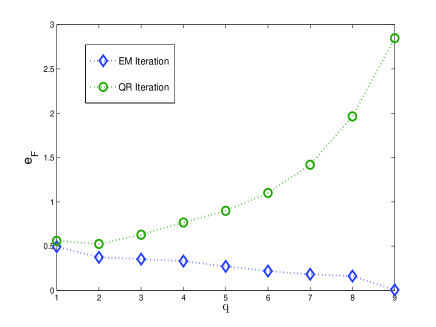
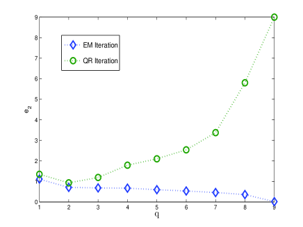
(a)   $e_{F}$ vs. $q$	(b)   $e_{2}$ vs. $q$

Figure 1: (a) The errors between ${\bf M}^{-1}$ and its approximate ${\bf A}{\bf A}^{T}+\delta{\bf I}_{m}$ where ${\bf A}$ and $\delta$ were estimated by the EM method and the QR method respectively, for $q=1,\ldots,9$.

Let us see the estimates of ${\bf A}$ in the cases that $q=1$ and $q=3$. First, when $q=1$, the EM estimate of ${\bf A}$ is

$${\bf A}=(-0.9563,-0.9790,-0.9126,-0.9774,-0.9308,-0.6513,-0.9108,-0.9579,-0.8809,-1.0007)^{T}.$$

It is further seen that ${\bf A}({\bf A}^{T}{\bf A})^{-\frac{1}{2}}=(-0.3285,-0.3363,-0.3135,-0.3357,-0.3197,-0.2237,\\ -0.3128,-0.3290,-0.3026,-0.3437)^{T}$ is the principal eigenvector of ${\bf M}$.

When $q=3$, the matrix ${\bf U}_{3}$ of the first three eigenvectors of ${\bf M}$ and the EM estimate of ${\bf A}({\bf A}^{T}{\bf A})^{-\frac{1}{2}}$ are respectively given by

$${\bf U}_{3}=\begin{bmatrix}-0.3285&0.4057&0.1792\\ -0.3363&-0.1540&-0.4530\\ -0.3135&-0.0746&0.0302\\ -0.3357&-0.3073&0.1697\\ -0.3197&0.3362&0.1897\\ -0.2237&0.4044&0.1239\\ -0.3128&-0.0221&0.1241\\ -0.3290&0.2035&0.0465\\ -0.3026&-0.6230&0.4150\\ -0.3437&-0.0711&-0.7013\end{bmatrix}\;\mbox{ and }\;{\bf A}({\bf A}^{T}{\bf A})^{-\frac{1}{2}}=\begin{bmatrix}0.1658&-0.3889&-0.3549\\ 0.3884&-0.1290&0.4159\\ 0.0359&-0.2973&0.1226\\ -0.1863&-0.3615&0.2647\\ 0.1194&-0.3819&-0.3019\\ 0.1769&-0.2709&-0.3525\\ -0.0128&-0.3352&0.0344\\ 0.1695&-0.3296&-0.1203\\ -0.5560&-0.4134&0.4152\\ 0.6341&-0.0423&0.4610\end{bmatrix}$$

It is easily verified that

$${\bf A}({\bf A}^{T}{\bf A})^{-\frac{1}{2}}={\bf U}_{3}{\bf V}$$

where

$${\bf V}=\left[\begin{array}[]{ccc}-0.3130&0.9214&-0.2304\\ 0.5098&-0.0417&-0.8593\\ -0.8013&-0.3864&-0.4566\end{array}\right]$$

is a $3{\times}3$ orthogonal matrix. This is in line with the theoretical justification given in Section 4.

In the case that $q=3$, we also implement the incomplete Cholesky decomposition of ${\bf M}$ as ${\bf M}\approx{\bf L}{\bf L}^{T}$ where ${\bf L}$ and ${\bf L}({\bf L}^{T}{\bf L})^{-\frac{1}{2}}$ are given as

$${\bf L}=\begin{bmatrix}0.6391&0.2092&1.16727\\ 0.7028&0.3565&0.2924\\ 0.6786&0.3931&0.3103\\ 0.6786&0.4302&0.2458\\ 0.6202&0.2184&0.4694\\ 0.4284&0.0659&0.4621\\ 0.6359&0.3751&0.3331\\ 0.6752&0.2549&0.4286\\ 0.6110&1.2587&0\\ 1.4017&0&0\end{bmatrix}\;\mbox{ and }\;{\bf L}({\bf L}^{T}{\bf L})^{-\frac{1}{2}}=\begin{bmatrix}0.0633&0.0016&0.8150\\ 0.2621&0.1315&0.0757\\ 0.2365&0.1659&0.0948\\ 0.2428&0.1977&0.0407\\ 0.2051&0.0321&0.2437\\ 0.1292&-0.0505&0.2843\\ 0.2108&0.1598&0.1236\\ 0.2379&0.0512&0.1968\\ 0.0816&0.8915&-0.1696\\ 0.8037&-0.2992&-0.3104\end{bmatrix}.$$

Assume that $\mathrm{range}({\bf L}({\bf L}^{T}{\bf L})^{-\frac{1}{2}})=\mathrm{range}({\bf U}_{3})$. Then we have ${\bf L}({\bf L}^{T}{\bf L})^{-\frac{1}{2}}={\bf U}_{3}{\bf R}$ where

$${\bf R}={\bf U}_{3}^{T}{\bf L}({\bf L}^{T}{\bf L})^{-\frac{1}{2}}=\begin{bmatrix}0.6248&-0.5466&0.4554\\ -0.6634&-0.5633&0.3665\\ 0.16903&-0.5628&-0.6421\end{bmatrix}.$$

We further have ${\bf I}_{3}=({\bf L}^{T}{\bf L})^{-\frac{1}{2}}{\bf L}^{T}{\bf L}({\bf L}^{T}{\bf L})^{-\frac{1}{2}}={\bf R}^{T}{\bf U}_{3}^{T}{\bf U}_{3}{\bf R}={\bf R}^{T}{\bf R}$. However, it is directly computed that ${\bf R}^{T}{\bf R}\neq{\bf I}_{3}$, yielding a conflict. This implies that the assumption $\mathrm{range}({\bf L}({\bf L}^{T}{\bf L})^{-\frac{1}{2}})=\mathrm{range}({\bf U}_{3})$ is not true. Thus, this example shows that the incomplete Cholesky decomposition can not be used to find the top eigenvectors of an arbitrary positive definite matrix.

Additionally, we defined a new positive definite matrix ${\bf K}$ as

$${\bf K}={\bf M}+\alpha^{2}{\bf I}_{10},$$

which has an explicit form as in (4). As mentioned in Section 4, we employed the incomplete Cholesky decomposition to approximate ${\bf K}^{-1}$. In particular, we first obtained the incomplete Cholesky decomposition of ${\bf M}$ as ${\bf M}\approx{\bf L}{\bf L}^{T}$ and then computed $(\alpha^{2}{\bf I}_{10}+{\bf L}{\bf L}^{T})^{-1}=\alpha^{-2}{\bf I}_{10}-\alpha^{-2}{\bf L}(\alpha^{2}{\bf I}_{q}+{\bf L}^{T}{\bf L})^{-1}{\bf L}^{T}$ as the approximation to ${\bf K}^{-1}$. Let $q=3$. We took $\alpha^{2}=0.1$ and $\alpha^{2}=0.0001$ to implement the empirical analysis. When $\alpha^{2}=0.1$, $e_{F}$ and $e_{2}$ with the incomplete Cholesky decomposition are respectively $7.0688$ and $14.8785$; $e_{F}$ and $e_{2}$ with our method are $0.3030$ and $0.5886$. When $\alpha^{2}=0.0001$, $e_{F}$ and $e_{2}$ with the incomplete Cholesky decomposition are respectively $7.0680{\times}10^{3}$ and $1.4877{\times}10^{4}$; $e_{F}$ and $e_{2}$ with our method are $0.3522$ and $0.6840$. This shows that the incomplete Cholesky decomposition fails when $\alpha^{2}$ takes a very small value. However, our method is numerically stable in every case. The reason is in that our method makes ${\bf A}{\bf A}^{T}{+}\delta{\bf I}_{10}$ better-conditioned than ${\bf K}$. But we see that ${\bf L}{\bf L}^{T}{+}\alpha^{2}{\bf I}_{10}$ is more ill-conditioned than ${\bf K}$.

Finally, we performed a simulation on a cluster to further validate efficiency of our approach in inverting large-size matrices. We randomly generated a $50000\times 50000$ positive definite matrix ${\bf M}$ from Wishart distribution $W_{50000}(50020,\mbox{\boldmath$\Sigma$\unboldmath})$ where $\mbox{\boldmath$\Sigma$\unboldmath}=0.5{\bf 1}_{50000}{\bf 1}_{50000}^{T}+0.5{\bf I}_{50000}$. The running time of the direct computation for ${\bf M}^{-1}$ is $5.4416\times 10^{4}$ (s), while our approximate approach with $q=224$ ($\approx\sqrt{50000}$) took $2.5452{\times}10^{3}$ seconds. Moreover, the errors are $e_{f}=0.9744$ and $e_{2}=2.4798$, respectively.

6.2 The Matrix Ridge Approximation for Spectral Clustering

The matrix ridge approximation (RA) with the EM iteration has potentially wide applications in those methods who involve the inversion or SD of a large-scale positive semidefinite matrix. In this section we apply RA to spectral clustering.

Spectral clustering (Shi and Malik, 2000, Ng et al., 2001) is a method for partitioning data into classes by relaxing an intractable partitioning problem into a tractable eigenvector problem, specifically a problem that can be reduced to the eigenvector problem in (5) for a particular matrix ${\bf M}$ (Zhang and Jordan, 2008). The solution of the relaxation is then “rounded” to yield a partition, where standard rounding methods include $K$-means and Procrustes analysis (Zhang and Jordan, 2008).

In the following experiments, we used the EM-based RA methods to solve the eigenvector relaxation associated with spectral clustering, and compared the results with the conventional direct spectral decomposition (SD) method. We also implemented the $K$-means and Procrustean transformation (PT) rounding algorithms given in Zhang and Jordan (2008) to obtain complete spectral clustering algorithms. This yields four spectral clustering algorithms, which we refer to as RA-KM, SD-KM, RA-PT and SD-PT.

Assume we are given a dataset $\{{\bf x}_{1},\ldots,{\bf x}_{m}\}$. We defined ${\bf M}$ as a kernel matrix ${\bf K}$ via the RBF kernel with single parameter $\beta$, i.e., $[{\bf K}]_{ij}=K({\bf x}_{i},{\bf x}_{j})=\exp({-}{\|{\bf x}_{i}-{\bf x}_{j}\|^{2}}/{\beta})$. Let ${\bf P}={\bf I}_{m}{-}\frac{1}{m}{\bf 1}_{m}{\bf 1}_{m}^{T}$ (i.e., ${\bf b}=\frac{1}{\sqrt{m}}{\bf 1}_{m}$). We then formed the $m{\times}m$ matrix ${\bf T}={\bf P}{\bf K}{\bf P}$, whose top $q$ eigenvectors are the solution of the eigenvector problem in (5). That is, the top $q$ eigenvectors of ${\bf T}$ are just the eigenvector relaxation associated with spectral clustering. Recall that $\hat{{\bf A}}(\hat{{\bf A}}^{T}\hat{{\bf A}})^{-\frac{1}{2}}={\bf U}_{q}{\bf V}=\widehat{{\bf X}}$, which implies that RA-KM and RA-PT employ the EM-based RA to find such $q$ eigenvectors. However, SD-KM and SD-PT employ the standard direct SD to obtain the $q$ eigenvectors.

We conducted the experiments on eight publicly available datasets from the UCI Machine Learning Repository: the dermatology data, the soybean data, the “A-J” letter data, the image segmentation data, the NIST optical handwritten digit data, the CTG (Cardiotocograms) data, the pen-based recognition of handwritten digits data, and the Statlog (Landsat Satellite) data. Table 6 gives a summary of these datasets.

In the clustering setup, $q{+}1$ is the number of classes. We initialized $K$-means by the orthogonal initialization method in Ng et al. (2001) and the Procrustean transformation by ${\bf I}_{q}$. The values of $\beta$ that we used are given in the last row of Table 3; they were set to be empirically optimal for these algorithms.

Table 3: Summary of the benchmark datasets: $m$—# of samples; $p$—# of features; $q{+}1$—# of classes; $\beta$—parameter in the kernel function $K(\cdot,\cdot)$.

	Derma	Soybean	Letter	CTG	Segmen	NIST	Landsat	Pen
$m$	$358$	$630$	$1978$	$2126$	$2310$	$3823$	$4435$	$7494$
$p$	$34$	$35$	$16$	$23$	$18$	$59$	$36$	$16$
$q{+}1$	$6$	$19$	$10$	$10$	$7$	$10$	$7$	$10$
$\beta$	$100$	$100$	$100$	$100$	$1000$	$1000$	$5000$	$100$

To evaluate the performance of the various clustering algorithms, we employed the Rand index (RI) (Rand, 1971). Given a set of $m$ samples ${\cal X}=\{{\bf x}_{1},\ldots,{\bf x}_{m}\}$, suppose that ${\cal U}=\{{\cal U}_{1},\ldots,{\cal U}_{r}\}$ and ${\cal V}=\{{\cal V}_{1},\ldots,{\cal V}_{s}\}$ are two different partitions of the samples in ${\cal X}$ such that $\cup_{i=1}^{r}{\cal U}_{i}={\cal X}=\cup_{j=1}^{s}{\cal V}_{j}$ and ${\cal U}_{i}\cap{\cal U}_{i^{\prime}}=\emptyset={\cal V}_{j}\cap{\cal V}_{j^{\prime}}$ for $i\neq i^{\prime}$ and $j\neq j^{\prime}$. Let $a$ be the number of pairs of samples that are in the same set in ${\cal U}$ and in the same set in ${\cal V}$, and $b$ the number of pairs of samples that are in different sets in ${\cal U}$ and in different sets in ${\cal V}$. The RI is given by $\mathrm{RI}=(a+b)/{m\choose 2}$. If $\mathrm{RI}=1$, the two partitions are identical. Since the true partitions are available for our datasets, we calculated the RI between the true partition and the partition obtained from each clustering algorithm.

We conducted 50 replicates of each of those algorithms with $K$-means rounding because of the random initialization required by $K$-means (this is not necessary for the Procrustean transformation, because it is initialized to the identity matrix). The results shown in Table 4 are based on the average of these 50 realizations.

From Table 4 we see that the clustering methods based on RA and SD have the almost same clustering performance. In Table 5 we reported the CPU times of the direct SD method and the EM-based RA method for computing the top $q$ eigenvectors. We see that RA method can be significantly more efficient than the SD method for large $m$, and this is borne out by our results. For example, on pen-based recognition of handwritten digits data ($m=7494$), the direct SD method takes twenty two minutes, the EM-based RA method only needs about four minutes.

Table 4: Rand Index (%).

	SD-PT	RA-PT	SD-KM	RA-KM
Derma	${95.49}$	${95.49}$	$94.57$ ($\pm 1.89$)	$94.47$ ($\pm 3.41$)
Soybean	$92.69$	${92.87}$	$91.32$ ($\pm 1.22$)	$91.80$ ($\pm 0.98$)
Letter	$85.68$	${85.63}$	$84.96$ ($\pm 0.49$)	$84.96$ ($\pm 0.43$)
CTG	$85.68$	${85.63}$	$84.96$ ($\pm 0.49$)	$84.96$ ($\pm 0.43$)
Segmen	$80.51$	$81.32$	${75.05}$ ($\pm 3.3$)	${79.00}$($\pm 2.27$)
NIST	${89.90}$	${89.89}$	$89.52$ ($\pm 0.70$)	$89.51$ ($\pm 0.63$)
Landsat	${84.88}$	${84.90}$	$83.33$ ($\pm 0.63$)	$83.28$ ($\pm 0.66$)
Pen	$90.61$	$90.64$	${91.14}$ ($\pm 0.48$)	${91.07}$($\pm 0.52$)

Table 5: CPU times (s) of running the spectral relaxation with the direct SD and EM-based ridge approximation (RA) which are performed in Matlab on a Core 2 Duo computer with a 2.27 GHz CPU and 8 GB of RAM.

	Derma	Soybean	Letter	CTG	Segmen	NIST	Landsat	Pen
SD	$0.2202$	$0.9148$	$28.3251$	$32.9942$	$35.2645$	$212.1458$	$289.9903$	$1361.8$
RA	$0.1862$	$0.7485$	$7.8297$	$9.4303$	$11.1811$	$42.7599$	$64.054$	$266.9177$

6.3 The Matrix Ridge Approximation for GPR

In this section we applied the matrix ridge approximation with the EM iteration to Gaussian process regression (GPR), and compared with the Nyström method (Williams and Seeger, 2001) and the incomplete Cholesky decomposition method (Fine et al., 2001).

Assume we are given a training dataset ${\mathcal{D}}=\{({\bf x}_{1},y_{1}),\ldots,({\bf x}_{m},y_{m})\}$, where the ${\bf x}_{i}\in{\mathbb{R}}^{p}$ are the input vectors and $y_{i}\in{\mathbb{R}}$ are the corresponding outputs. In the GPR model $y$ is defined as

$$y=u+f({\bf x})+\epsilon,\quad\epsilon\thicksim N(0,\sigma^{2}),$$

where $f({\bf x})$ follows a Gaussian process with mean function 0 and covariance function $K(\cdot,\cdot)$. This implies that ${\bf f}=(f({\bf x}_{1}),f({\bf x}_{2}),\ldots,f({\bf x}_{m}))^{T}$, corresponding outputs of the input vectors in the training dataset ${\mathcal{D}}$, has multivariate Gaussian distribution $N({\bf 0},{\bf K})$, where ${\bf K}$ is the $m{\times}m$ covariance matrix with $[{\bf K}]_{ij}=K({\bf x}_{i},{\bf x}_{j})$.

We employed the Gaussian RBF kernel function $K(\cdot,\cdot)$ with a separate length-scale parameter for each variate of the input vector, plus the signal and noise variance parameters $\sigma_{f}^{2}$ and $\sigma^{2}$. These parameters are trained by optimizing the marginal likelihood on a subset of the training data. Here we ignored the learning details and directly used the code provided by Rasmussen and Williams (2006) to implement the training. We concentrated our attention on the test procure.

For a test input vector ${\bf x}_{*}$, the prediction of the corresponding output $y_{*}$ is based on the conditional posterior distribution $p(y_{*}|{\bf y})$, which is also Gaussian. In particular, the predicted mean at ${\bf x}_{*}$ is given by

$$\hat{y}_{*}={\bf k}^{T}({\bf x}_{*})({\bf K}{+}\sigma^{2}{\bf I}_{m})^{-1}{\bf y},$$

where ${\bf y}=(y_{1},\ldots,y_{m})^{T}$ and ${\bf k}({\bf x}_{*})=(K({\bf x}_{*},{\bf x}_{1}),\ldots,K({\bf x}_{*},{\bf x}_{m}))^{T}$ (see, Rasmussen and Williams, 2006). As we can see, GPR requires us to compute the inverse of ${\bf K}{+}\sigma^{2}{\bf I}_{m}$, which is an $m{\times}m$ positive definite matrix. When the size ($m$) of the training dataset is very large, this limits the efficient application of GPR.

Since ${\bf K}{+}\sigma^{2}{\bf I}_{m}$ has the explicit form mentioned in Section 4, Williams and Seeger (2001) considered the Nyström approximation for its inverse when $m$ is large. The Nyström method randomly chooses $q$ columns of ${\bf K}$ without replacement. Let ${\bf K}_{m,q}$ denote the $m{\times}q$ matrix consisting of such $q$ columns. Then the Nyström approximation of ${\bf K}$ is ${\bf K}_{m,q}{\bf K}_{q,q}^{-1}{\bf K}_{m,q}^{T}$. Here we also compared the approximate method based on the incomplete Cholesky decomposition; that is, we first implemented the incomplete Cholesky decomposition of ${\bf K}$ as ${\bf K}\approx{\bf L}{\bf L}^{T}$ where ${\bf L}$ is an $m{\times}q$ lower triangular matrix. After having obtained the Nyström approximation or the incomplete Cholesky decomposition, we then computed $({\bf K}_{m,q}{\bf K}_{q,q}^{-1}{\bf K}_{m,q}^{T}{+}\sigma^{2}{\bf I}_{m})^{-1}$ or $({\bf L}{\bf L}^{T}{+}\sigma^{2})^{-1}{\bf I}_{m}$ via the Sherman-Morrison-Woodbury formula. Recall that we applied the ridge approximation directly on ${\bf K}{+}\sigma^{2}{\bf I}_{m}$, rather than on ${\bf K}$.

We conducted the experiments on seven publicly available datasets from the UCI Machine Learning Repository: the Boston Housing data, the Concrete Compressive Strength (CCS) data, the Contraceptive Method Choice (CMC) data, the Abalone data, the Landsat Satellite (Sat) data, the SARCOS data, and the YearPredictionMSD (YPMSD) data. We employed the setting given in the UCI Machine Learning Repository for training and testing for the first six datasets. For the YPMSD data, we employed two settings for training and testing. In the first setting (YPMSD1) we used the first $60,000$ samples for training and the rest of the samples for testing, while in the second setting (YPMSD2) we used the first $100,000$ samples for training and the rest of the samples for testing. Table 6 gives a summary of these datasets.

Table 6: Summary of the datasets: $m$—# of training samples; $n$—# of test samples; $p$—# of features;

	Housing	CCS	CMC	Abalone	Sat	SARCOS	YPMSD1	YPMSD2
$m$	$455$	$700$	$1,000$	$3,133$	$4,435$	$5,000$	60,000	$100,000$
$n$	$51$	$330$	$473$	$1,044$	$2,000$	$4,449$	455,345	415,3455
$p$	$13$	$8$	$9$	$8$	$36$	$21$	90	$90$

We evaluated the performance of predictions using the standardized mean squared error (SMSE) (Rasmussen and Williams, 2006). We set the rank of the matrix ${\bf A}$ in the ridge approximation, the columns of the matrix ${\bf L}$(${\bf K}\approx{\bf L}{\bf L}^{T}$) in the incomplete Cholesky decomposition, and the columns uniformly sampled from the original kernel matrix in the Nyström method to the same number $q$. We then compared the performance of the three methods.

For the Nyström method, for each given $q$, we repeated the experiment 50 times. We found that the results are very sensitive to the columns randomly selected. The method works well in a few instances, but in most cases its performance is extremely poor. Thus, given $q$, we reported the smallest SMSE for the Nyström method.

Figure 2 shows SMSE values over the first six datasets. It should be worth pointing out that the performance of the Nyström method is very poor on the Sat and CCS datasets. Thus, we omitted the SMSE values on the two datasets for the Nyström method. Also, when $q$ is less than 4396 for the Sat dataset, the performance of the incomplete Cholesky decomposition method is poor. For this reason, we also omitted the SMSE values for the incomplete Cholesky decomposition method on the Sat dataset.

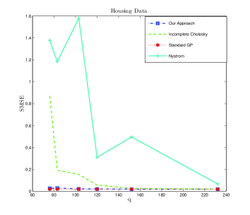
(a) Housing Data

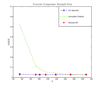
(b) Concrete Compressive Strength Data

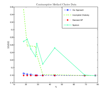
(c) Contraceptive Method Choice Data

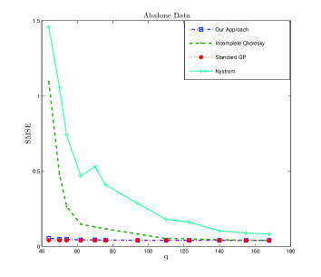
(d) Abalone Data

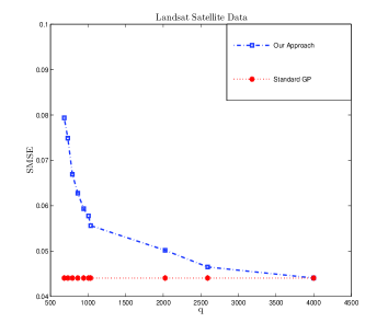
(e) Landsat Satellite Data

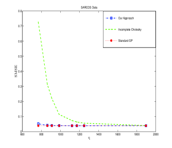
(f) SARCOS Data

Figure 2: Comparisons of the ridge approximation method, the Nyström method and the incomplete Cholesky decomposition method.

From Figure 2, we see that the performance of the ridge approximation method is nearly the same as that of standard GPR. Moreover, the ridge approximation is not sensitive to the value of $q$. For a wide range of $q$, the GPR prediction varies very little. When $q$ takes a small value, the ridge approximation still works well. Contrarily, when $q$ is small, the incomplete Cholesky decomposition is not very effective, because it results in an underfitting problem in which ${\bf L}{\bf L}^{T}{+}\sigma^{2}{\bf I}_{m}$ is ill-conditioned. However, the ridge approximation can avoid this problem, because it makes ${\bf A}{\bf A}^{T}{+}\delta{\bf I}_{m}$ better-conditioned than ${\bf K}$ itself (see the discussion in Section 6.1).

For the YPMSD data, we did not include the results with the Nyström method and the incomplete Cholesky decomposition method because the performance of these two methods is very poor when $q\ll m$ (e.g., $q\leq\sqrt{m}$). We only took $q=245$ for YPMSD1 and $q=316$ for YPMSD2 ($\approx\sqrt{m}$) to implement the ridge approximation method. Since the size of the matrix ${\bf K}+\sigma^{2}{\bf I}_{m}$ is too large, we partitioned it into the $2{\times}2$ block submatrices in the direct computation of $({\bf K}+\sigma^{2}{\bf I}_{m})^{-1}$. Although this does not reduce the computational cost, it can make the computation more numerically stable. To reduce the storage space of data, all computations were carried out with single precision in Matlab. However, we still could not complete the experiment with the direct computation method on the YPMSD2 dataset due to limited storage space.

The SMSE values with the direct method and the ridge approximation method for computing $({\bf K}+\sigma^{2}{\bf I}_{m})^{-1}$ on YPMSD1 are $3.7713{\times}10^{-5}$ and $2.9232{\times}10^{-5}$, respectively. We see that the ridge approximation slightly outperforms the direct computation. We hypothesize that this phenomenon is a result of roundoff error in the floating point computations. The SMSE value with the ridge approximation on YPMSD2 is $2.8959{\times}10^{-5}$. Therefore, the ridge approximation method is effective.

Finally, in Table 7 we report the running times with our matrix ridge approximation and the direct calculation for $({\bf K}+\sigma^{2}{\bf I}_{m})^{-1}$ on the datasets. The reported results with our method are based on that $q$ is taken as the integer closest to $\sqrt{m}$. We see that our method is able to reduce computation when $m$ is vary large. For example, on the YPMSD1 dataset the direct computation took $1.2436{\times}10^{5}$ seconds, while the ridge approximation took $5.814{\times}10^{3}$ seconds. In summary, our proposed approach is efficient and effective.

Table 7: CPU times (s) of running the test procedure of GPR with the direct computation and EM-based ridge approximation (RA) which are performed in Matlab on a Workstation with a 3.07 GHz CPU and 24 GB of RAM.

	Housing	CCS	CMC	Abalone	Sat	SARCOS	YPMSD1	YPMSD2
Direct	$0.7020$	$0.5460$	$0.7644$	$33.8210$	$105.0823$	$145.8141$	$1.2436{\times}10^{5}$	NA
EM-RA	$0.1872$	$0.530$	$0.9048$	$9.8437$	$18.7981$	$20.8729$	$5.814{\times}10^{3}$	$1.0664{\times}10^{5}$

7 Conclusion

In this paper we have proposed the matrix ridge approximation method, which tries to find an approximation for a symmetric positive semidefinite matrix. We have also developed probabilistic formulations for this method. The probabilistic formulation not only provides a statistical interpretation but also leads us to an efficient EM iterative procedure for the matrix ridge approximation. The matrix ridge approximation with the EM iteration has potentially broad applicability in machine learning problems that involve the inversion or spectral decomposition of a large-scale positive semidefinite matrix. In particular, we have empirically illustrated the effectiveness and efficiency of the matrix ridge approximation in the case of spectral clustering and Gaussian process regression.

The support vector machine (SVM) and Gaussian process classification (GPC) are two classical kernel classification methods. When applying them to large-scale data sets, we also meet a computational challenge. The matrix ridge approximation technique is a potentially useful approach for handling this challenge. We will study this issue in future work. Recall that each EM iteration for the matrix ridge approximation takes time $O(m^{2}q)$ and it mainly involves matrix multiplications. To make the method more efficient, we can consider the parallel implementation of the matrix multiplications.

A Several Lemmas

In order to prove the theorems, we first present several lemmas that will be used.

Lemma 4

Suppose ${\bf B}\in{\mathbb{R}}^{m{\times}m}$. Let $c_{i}+\imath d_{i}$ for $i=1,\ldots,m$ be the eigenvalues of ${\bf B}$ where $\imath^{2}=-1$ and the $c_{i},d_{i}\in{\mathbb{R}}$. Then,

1. $\mathrm{tr}({\bf B})=\sum_{i=1}^{m}c_{i}$ and $\mathrm{tr}({\bf B}^{2})=\sum_{i=1}^{m}(c^{2}_{i}-d_{i}^{2})$ .

2. $\sum_{i=1}^{m}c_{i}^{2}+d_{i}^{2}\leq\mathrm{tr}({\bf B}{\bf B}^{T})$, $\sum_{i=1}^{m}c_{i}^{2}\leq\frac{1}{2}\mathrm{tr}({\bf B}{\bf B}{+}{\bf B}{\bf B}^{T})$, and $\sum_{i=1}^{m}d_{i}^{2}\leq\frac{1}{2}\mathrm{tr}({\bf B}{\bf B}^{T}{-}{\bf B}{\bf B})$.

Proof  It is obvious that $c_{i}+\imath d_{i}$ is the eigenvalue of ${\bf B}$ iff $c_{i}-\imath d_{i}$ is the eigenvalue of ${\bf B}$. Accordingly, we have Part (i).

In addition, let the Schur factorization of ${\bf B}$ be ${\bf B}={\bf Q}{\bf T}{\bf Q}^{*}$ where ${\bf Q}$ is unitary and ${\bf T}$ is upper-triangular with the eigenvalues of ${\bf B}$ at the diagonals. Thus,

$$\mathrm{tr}({\bf B}{\bf B}^{T})=\mathrm{tr}({\bf T}{\bf T}^{*})\geq\sum_{i=1}^{m}(c_{i}+\imath d_{i})(c_{i}-\imath d_{i})=\sum_{i=1}^{m}(c_{i}^{2}+d_{i}^{2}).$$

In addition, we also have

$$\frac{1}{2}\mathrm{tr}({\bf B}{\bf B}^{T}+{\bf B}{\bf B})=\frac{1}{4}\mathrm{tr}(({\bf T}+{\bf T}^{*})({\bf T}+{\bf T}^{*}))\geq\sum_{i=1}^{m}c_{i}^{2}$$

and

$$\frac{1}{2}\mathrm{tr}({\bf B}{\bf B}^{T}-{\bf B}{\bf B})=\frac{1}{4}\mathrm{tr}(({\bf T}-{\bf T}^{*})({\bf T}-{\bf T}^{*}))\geq\sum_{i=1}^{m}d_{i}^{2}.$$

The proof completes.  

We now turn to our proposed approach and follow the notations in Table 1. Without loss of generality, we only consider the case that ${\bf b}\neq 0$ and ${\bf b}^{T}{\bf b}=1$. In this case, ${\bf P}={\bf I}_{m}-{\bf b}{\bf b}^{T}$ is idempotent, symmetric and of rank $m{-}1$. Thus we can express it as ${\bf P}=\mbox{\boldmath$\Psi$\unboldmath}\left[\begin{array}[]{cc}{\bf I}_{m{-}1}&{\bf 0}\\ {\bf 0}&{\bf 0}\end{array}\right]\mbox{\boldmath$\Psi$\unboldmath}^{T}$ where $\mbox{\boldmath$\Psi$\unboldmath}^{T}\mbox{\boldmath$\Psi$\unboldmath}=\mbox{\boldmath$\Psi$\unboldmath}\mbox{\boldmath$\Psi$\unboldmath}^{T}={\bf I}_{m}$. Let $\mbox{\boldmath$\Psi$\unboldmath}_{1}$ be an $m{\times}(m{-}1)$ matrix containing the first $m{-}1$ columns of $\Psi$. Then $\mbox{\boldmath$\Psi$\unboldmath}=[\mbox{\boldmath$\Psi$\unboldmath}_{1},{\bf b}]$ so that $\mbox{\boldmath$\Psi$\unboldmath}_{1}^{T}\mbox{\boldmath$\Psi$\unboldmath}_{1}={\bf I}_{m{-}1}$, $\mbox{\boldmath$\Psi$\unboldmath}_{1}^{T}{\bf b}={\bf 0}$ and ${\bf P}=\mbox{\boldmath$\Psi$\unboldmath}_{1}\mbox{\boldmath$\Psi$\unboldmath}_{1}^{T}$.

In order to prove the theorems given in Section 3, we use the same notation as in Section 3. Moreover, we here and later denote ${\bf Z}=\mbox{\boldmath$\Psi$\unboldmath}_{1}^{T}{\bf A}$ ($(m{-}1){\times}q)$), ${\bf G}=\mbox{\boldmath$\Psi$\unboldmath}_{1}^{T}{\bf T}\mbox{\boldmath$\Psi$\unboldmath}_{1}=\mbox{\boldmath$\Psi$\unboldmath}_{1}^{T}{\bf P}{\bf M}{\bf P}\mbox{\boldmath$\Psi$\unboldmath}_{1}=\mbox{\boldmath$\Psi$\unboldmath}_{1}^{T}{\bf M}\mbox{\boldmath$\Psi$\unboldmath}$ ($(m{-}1){\times}(m{-}1)$) and $\mbox{\boldmath$\Theta$\unboldmath}=\mbox{\boldmath$\Psi$\unboldmath}_{1}^{T}\mbox{\boldmath$\Omega$\unboldmath}\mbox{\boldmath$\Psi$\unboldmath}_{1}=\mbox{\boldmath$\Psi$\unboldmath}_{1}^{T}({\bf A}{\bf A}^{T}+\delta{\bf I}_{m})\mbox{\boldmath$\Psi$\unboldmath}_{1}={\bf Z}{\bf Z}^{T}+\delta{\bf I}_{m{-}1}$ ($(m{-}1){\times}(m{-}1)$). With these notations, we present the following several lemmas.

Lemma 5

Let $\lambda({\bf C})$ be the set of the all eigenvalues of ${\bf C}$. Then $\lambda({\bf T})=\lambda({\bf G})\cup\{0\}$. Furthermore, if $\phi$ is the eigenvector of ${\bf G}$ associated with its eigenvalue $\gamma$, then $\mbox{\boldmath$\Psi$\unboldmath}_{1}\mbox{\boldmath$\phi$\unboldmath}$ is the eigenvector of ${\bf T}$ associated with its eigenvalue $\gamma$. Conversely, if ${\bf u}$ satisfying ${\bf u}^{T}{\bf b}=0$ is the eigenvector of ${\bf T}$ associated with its eigenvalue $\gamma$, then $\mbox{\boldmath$\Psi$\unboldmath}_{1}^{T}{\bf u}$ is the eigenvector of ${\bf G}$ associated with its eigenvalue $\gamma$.

Proof  Recall that

$${\bf T}={\bf P}{\bf T}{\bf P}=\mbox{\boldmath$\Psi$\unboldmath}\left[\begin{array}[]{cc}\mbox{\boldmath$\Psi$\unboldmath}_{1}^{T}{\bf T}\mbox{\boldmath$\Psi$\unboldmath}_{1}&{\bf 0}\\ {\bf 0}&0\end{array}\right]\mbox{\boldmath$\Psi$\unboldmath}^{T}=\mbox{\boldmath$\Psi$\unboldmath}\left[\begin{array}[]{cc}{\bf G}&{\bf 0}\\ {\bf 0}&0\end{array}\right]\mbox{\boldmath$\Psi$\unboldmath}^{T}.$$

Thus, $\lambda({\bf T})=\lambda({\bf G})\cup\{0\}$. Letting ${\bf G}\mbox{\boldmath$\phi$\unboldmath}=\gamma\mbox{\boldmath$\phi$\unboldmath}$, we have

$${\bf S}\mbox{\boldmath$\Psi$\unboldmath}_{1}\mbox{\boldmath$\phi$\unboldmath} = \mbox{\boldmath$\Psi$\unboldmath}\left[\begin{array}[]{cc}{\bf G}&{\bf 0}\\ {\bf 0}&0\end{array}\right]\mbox{\boldmath$\Psi$\unboldmath}^{T}\mbox{\boldmath$\Psi$\unboldmath}_{1}\mbox{\boldmath$\phi$\unboldmath}=\mbox{\boldmath$\Psi$\unboldmath}\left[\begin{array}[]{cc}{\bf G}&{\bf 0}\\ {\bf 0}&0\end{array}\right]\left[\begin{array}[]{c}{\bf I}_{m{-}1}\\ 0\end{array}\right]\mbox{\boldmath$\phi$\unboldmath}$$

$$= \mbox{\boldmath$\Psi$\unboldmath}\left[\begin{array}[]{c}{\bf G}\\ 0\end{array}\right]\mbox{\boldmath$\phi$\unboldmath}=\mbox{\boldmath$\Psi$\unboldmath}\left[\begin{array}[]{c}{\bf I}_{m{-}1}\\ 0\end{array}\right]{\bf G}\mbox{\boldmath$\phi$\unboldmath}=\mbox{\boldmath$\Psi$\unboldmath}_{1}{\bf G}\mbox{\boldmath$\phi$\unboldmath}=\gamma\mbox{\boldmath$\Psi$\unboldmath}_{1}\mbox{\boldmath$\phi$\unboldmath},$$

which shows that $\mbox{\boldmath$\Psi$\unboldmath}_{1}\mbox{\boldmath$\phi$\unboldmath}$ is the eigenvectors of ${\bf T}$. Also, since

$${\bf G}\mbox{\boldmath$\Psi$\unboldmath}_{1}^{T}{\bf u}=\mbox{\boldmath$\Psi$\unboldmath}_{1}^{T}{\bf T}\mbox{\boldmath$\Psi$\unboldmath}_{1}\mbox{\boldmath$\Psi$\unboldmath}_{1}^{T}{\bf u}=\mbox{\boldmath$\Psi$\unboldmath}_{1}^{T}{\bf T}{\bf u}=\gamma\mbox{\boldmath$\Psi$\unboldmath}_{1}^{T}{\bf u}$$

$\mbox{\boldmath$\Psi$\unboldmath}_{1}^{T}{\bf u}$ is the eigenvector of ${\bf G}$ associated with its eigenvalue $\gamma$.  

Lemma 6

Assume that $k$ is an arbitrary integer. Then,

1. $\mbox{\boldmath$\Psi$\unboldmath}_{1}^{T}\mbox{\boldmath$\Omega$\unboldmath}^{-k}\mbox{\boldmath$\Psi$\unboldmath}_{1}=\mbox{\boldmath$\Theta$\unboldmath}^{-k}$, ${\bf b}^{T}\mbox{\boldmath$\Omega$\unboldmath}^{-k}\mbox{\boldmath$\Psi$\unboldmath}_{1}={\bf 0}$ and ${\bf b}^{T}\mbox{\boldmath$\Omega$\unboldmath}^{-k}{\bf b}=\delta^{-k}$;

2. $\mathrm{tr}(\mbox{\boldmath$\Omega$\unboldmath}^{-k})=\mathrm{tr}(\mbox{\boldmath$\Theta$\unboldmath}^{-k})+\delta^{-k}$.

Proof  As for (i), we first have

$$\mbox{\boldmath$\Psi$\unboldmath}_{1}^{T}\mbox{\boldmath$\Omega$\unboldmath}^{-1}\mbox{\boldmath$\Psi$\unboldmath}_{1} =\mbox{\boldmath$\Psi$\unboldmath}_{1}^{T}({\bf A}{\bf A}^{T}+\delta{\bf I}_{m})^{-1}\mbox{\boldmath$\Psi$\unboldmath}_{1}=\mbox{\boldmath$\Psi$\unboldmath}_{1}^{T}(\delta^{-1}{\bf I}_{m}-\delta^{-1}{\bf A}(\delta{\bf I}_{q}+{\bf A}^{T}{\bf A})^{-1}{\bf A}^{T})\mbox{\boldmath$\Psi$\unboldmath}_{1}$$

$$=\delta^{-1}{\bf I}_{m{-}1}-\delta^{-1}{\bf Z}(\delta{\bf I}_{q}+{\bf Z}^{T}{\bf Z})^{-1}{\bf Z}=(\delta{\bf I}_{m{-}1}+{\bf Z}{\bf Z})^{-1}=\mbox{\boldmath$\Theta$\unboldmath}^{-1}$$

due to ${\bf A}^{T}{\bf A}={\bf A}^{T}{\bf P}{\bf A}={\bf A}^{T}\mbox{\boldmath$\Psi$\unboldmath}_{1}\mbox{\boldmath$\Psi$\unboldmath}_{1}^{T}{\bf A}={\bf Z}^{T}{\bf Z}$. Assume that $\mbox{\boldmath$\Psi$\unboldmath}_{1}^{T}\mbox{\boldmath$\Omega$\unboldmath}^{1-l}\mbox{\boldmath$\Psi$\unboldmath}_{1}=\mbox{\boldmath$\Theta$\unboldmath}^{1-l}$ for some positive integer $l$. Then

$$\mbox{\boldmath$\Psi$\unboldmath}_{1}^{T}\mbox{\boldmath$\Omega$\unboldmath}^{-l}\mbox{\boldmath$\Psi$\unboldmath}_{1}=\mbox{\boldmath$\Psi$\unboldmath}_{1}^{T}\mbox{\boldmath$\Omega$\unboldmath}^{1-l}(\mbox{\boldmath$\Psi$\unboldmath}_{1}\mbox{\boldmath$\Psi$\unboldmath}_{1}^{T}+{\bf b}{\bf b}^{T})\mbox{\boldmath$\Omega$\unboldmath}^{-1}\mbox{\boldmath$\Psi$\unboldmath}_{1}=\mbox{\boldmath$\Theta$\unboldmath}^{-l}+\mbox{\boldmath$\Psi$\unboldmath}_{1}^{T}\mbox{\boldmath$\Omega$\unboldmath}^{1-l}{\bf b}{\bf b}^{T}\mbox{\boldmath$\Omega$\unboldmath}^{-1}\mbox{\boldmath$\Psi$\unboldmath}_{1}=\mbox{\boldmath$\Theta$\unboldmath}^{-l}$$

due to ${\bf b}^{T}\mbox{\boldmath$\Omega$\unboldmath}^{-1}\mbox{\boldmath$\Psi$\unboldmath}_{1}={\bf 0}$. Thus, we obtain $\mbox{\boldmath$\Psi$\unboldmath}^{T}\mbox{\boldmath$\Omega$\unboldmath}^{-k}\mbox{\boldmath$\Psi$\unboldmath}_{1}=\mbox{\boldmath$\Theta$\unboldmath}^{-k}$ by the induction. Similarly, we ${\bf b}^{T}\mbox{\boldmath$\Omega$\unboldmath}^{-k}\mbox{\boldmath$\Psi$\unboldmath}_{1}={\bf 0}$ and ${\bf b}^{T}\mbox{\boldmath$\Omega$\unboldmath}^{-k}{\bf b}=\delta^{-k}$.

Finally, it follows from (i) that

$$\mathrm{tr}(\mbox{\boldmath$\Omega$\unboldmath}^{-k})=\mathrm{tr}\left(\left[\begin{array}[]{c}\mbox{\boldmath$\Psi$\unboldmath}_{1}^{T}\\ {\bf b}^{T}\end{array}\right]\mbox{\boldmath$\Omega$\unboldmath}^{-k1}[\mbox{\boldmath$\Psi$\unboldmath}_{1},{\bf b}]\right)=\mathrm{tr}(\mbox{\boldmath$\Theta$\unboldmath}^{-k})+\delta^{-k}.$$

 

B Proof for Theorem 1

In order to prove Theorem 1, we present a more general alternative which is based on two variants of $F$ and $G$. In particular, the first variant is

$$F_{1}({\bf A},\delta)=\|{\bf M}{-}{\bf A}{\bf A}^{T}{-}\delta{\bf I}_{m}\|_{F}^{2}=\mathrm{tr}\big{(}({\bf M}{-}{\bf A}{\bf A}^{T}{-}\delta{\bf I}_{m})^{2}\big{)},$$

while the second variant is

$$G_{1}({\bf A},\delta)=\log|{\bf A}{\bf A}^{T}+\delta{\bf I}_{m}|+\mathrm{tr}(({\bf A}{\bf A}^{T}+\delta{\bf I}_{m})^{-1}{\bf M}).$$

Obviously, $F_{1}$ and $F$ (or $G_{1}$ and $G$) become identical when ${\bf b}={\bf 0}$. The minimizers of $F_{1}$ as well as $G_{1}$ are given in the following theorem.

Theorem 7

Let $\gamma_{1}\geq\cdots\geq\gamma_{q}\geq\cdots\geq\gamma_{m}$ ($\geq 0$) be the eigenvalues of ${\bf T}={\bf P}{\bf M}{\bf P}$, ${\bf V}$ be an arbitrary $q{\times}q$ orthogonal matrix, ${\mbox{\boldmath$\Gamma$\unboldmath}_{q}}$ be a $q{\times}q$ diagonal matrix containing the first $q$ principal (largest) eigenvalues $\gamma_{i}$, and ${{{\bf U}_{q}}}$ be an $n{\times}q$ column-orthonormal matrix in which the $q$ column vectors are the principal eigenvectors corresponding to ${\mbox{\boldmath$\Gamma$\unboldmath}_{q}}$. Assume that $\delta>0$ and that ${\bf A}\in{\mathbb{R}}^{m{\times}q}$ ($q<\min(m,p)$) is of full column rank and satisfies ${\bf A}^{T}{\bf b}={\bf 0}$. If the following conditions are satisfied

$$\gamma_{i}>\frac{1}{m{-}q}\Big{(}{\bf b}^{T}{\bf M}{\bf b}+\sum_{j=q{+}1}^{m}\gamma_{j}\Big{)},\quad\mbox{ for }i=1,\ldots,q,$$ (10)

then the strict local minimum of $F_{1}({\bf A},\delta)$ and $G_{1}({\bf A},\delta)$ w.r.t. $({\bf A},\delta)$ are respectively obtained when

$$\widehat{{\bf A}}={{\bf U}_{q}}({\mbox{\boldmath$\Gamma$\unboldmath}_{q}}-\hat{\delta}{\bf I}_{q})^{1/2}{\bf V}\quad\mbox{and}\quad\hat{\delta}=\frac{1}{m{-}q}\Big{[}{\bf b}^{T}{\bf M}{\bf b}+\sum_{j=q+1}^{m}\gamma_{j}\Big{]}.$$

Note that ${\bf P}{\bf S}{\bf P}={\bf S}$ and ${\bf b}^{T}{\bf S}{\bf b}=0$. Thus, when viewing ${\bf S}$ as ${\bf M}$ in Theorem 7, we immediately obtain Theorem 1 from Theorem 7.

Theorem 7 shows the connection between the estimates of ${\bf A}$ and $\delta$ based on the minimizations of $F_{1}$ and $G_{1}$. In particular, the estimates of ${\bf A}$ and $\delta$ via minimizing $F_{1}$ are equivalent to those of ${\bf A}$ and $\delta$ via minimizing $G_{1}$. We note that the minimizer $(\widehat{{\bf A}},\hat{\delta})$ of $G_{1}$ under ${\bf b}={\bf 0}$ was given in Magnus and Neudecker (1999). The conditions in (10) aim to ensure that $({\mbox{\boldmath$\Gamma$\unboldmath}_{q}}-\hat{\delta}{\bf I}_{q})^{1/2}$ exists and $\widehat{{\bf A}}$ is of full column rank. In the case that ${\bf b}={\bf 0}$, $\gamma_{q}>\gamma_{q{+}1}$ suffices for the conditions. In fact, they are always satisfied whenever there is at least one $\gamma_{j}$ where $j\in\{q{+}1,\ldots,m\}$ such that $\gamma_{q}>\gamma_{j}>0$. Thus, the conditions in (10) are trivial when ${\bf b}={\bf 0}$.

However, the conditions are not always satisfied when ${\bf b}^{T}{\bf b}=1$. For example, let

$${\bf M}=[{\bf b},\mbox{\boldmath$\Psi$\unboldmath}_{1}]\left[\begin{array}[]{cc}1+\alpha^{2}&{\bf 0}\\ {\bf 0}&\alpha^{2}{\bf I}_{m{-}1}\end{array}\right]\left[\begin{array}[]{c}{\bf b}^{T}\\ \mbox{\boldmath$\Psi$\unboldmath}_{1}^{T}\end{array}\right]$$

for $\alpha\neq 0$ such that $\mbox{\boldmath$\Psi$\unboldmath}_{1}^{T}{\bf b}={\bf 0}$ and $\mbox{\boldmath$\Psi$\unboldmath}_{1}^{T}\mbox{\boldmath$\Psi$\unboldmath}_{1}={\bf I}_{m{-}1}$. It is clear that ${\bf b}^{T}{\bf M}{\bf b}=1+\alpha^{2}$ and ${\bf T}={\bf P}{\bf M}{\bf P}=\alpha^{2}{\bf P}$. This implies that the eigenvalues $\gamma_{i}$ of ${\bf T}$ are $\alpha^{2}$ with multiplicity $m{-}1$ and $0$ with multiplicity 1. As a result, for any $i\leq q<m$, we always have

$$\gamma_{i}=\alpha^{2}<\alpha^{2}+1/(m-q)=\frac{1}{m{-}q}\Big{(}{\bf b}^{T}{\bf M}{\bf b}+\sum_{j=q{+}1}^{m}\gamma_{j}\Big{)}.$$

Thus, the condition in (10) is not satisfied. Consequently, this condition would limit the use of $F_{1}$ and $G_{1}$ in the matrix ridge approximation. This is the reason why we employ $F$ and $G$ instead of $F_{1}$ and $G_{1}$ respectively.

B.1 Proof for the Minimizer of $F_{1}({\bf A},\delta)$ w.r.t. $({\bf A},\delta)$

Consider the Lagrangian function of

$$L=\mathrm{tr}({\bf M}-{\bf A}{\bf A}^{T}-\delta{\bf I}_{m})^{2}+4{\bf b}^{T}{\bf A}{\bf a}$$

where ${\bf a}$ is a $q{\times}1$ vector of Lagrangian multipliers. We now compute

$$dL =-2\mathrm{tr}\big{[}({\bf M}-{\bf A}{\bf A}^{T}-\delta{\bf I}_{m})((d{\bf A}){\bf A}^{T}+{\bf A}(d{\bf A}^{T}))\big{]}+4{\bf b}^{T}(d{\bf A}){\bf a}$$

$$=-4\mathrm{tr}({\bf A}^{T}({\bf M}-{\bf A}{\bf A}^{T}-\delta{\bf I}_{m})(d{\bf A}))+4{\bf b}^{T}(d{\bf A}){\bf a},$$

$$dL =-2\mathrm{tr}({\bf M}-{\bf A}{\bf A}^{T}-\delta{\bf I}_{m})d\delta.$$

Using the first-order condition, we obtain

$$-{\bf A}^{T}({\bf M}-{\bf A}{\bf A}^{T}-\delta{\bf I}_{m})+{\bf a}{\bf b}^{T} ={\bf 0},$$

$$\mathrm{tr}({\bf M}-{\bf A}{\bf A}^{T}-\delta{\bf I}_{m}) =0.$$

Postmultiplying the above first equation by ${\bf b}$, we obtain ${\bf a}={\bf A}^{T}{\bf M}{\bf b}$ because of ${\bf A}^{T}{\bf b}={\bf 0}$. As a result, we have

$${\bf T}{\bf A}={\bf A}({\bf A}^{T}{\bf A}+\delta{\bf I}_{q}),$$

where ${\bf T}={\bf P}{\bf M}{\bf P}$. Assume the spectral decomposition of ${\bf A}^{T}{\bf A}$ as ${\bf A}^{T}{\bf A}={\bf V}\mbox{\boldmath$\Lambda$\unboldmath}{\bf V}^{T}$. Hence,

$${\bf T}{\bf A}{\bf V}\mbox{\boldmath$\Lambda$\unboldmath}^{-\frac{1}{2}}={\bf A}{\bf V}\mbox{\boldmath$\Lambda$\unboldmath}^{-\frac{1}{2}}(\mbox{\boldmath$\Lambda$\unboldmath}+\delta{\bf I}_{q}).$$

This implies that the diagonal elements of $\mbox{\boldmath$\Lambda$\unboldmath}+\delta{\bf I}_{q}$ are the $q$ eigenvalues of ${\bf T}$, and ${\bf A}{\bf V}\mbox{\boldmath$\Lambda$\unboldmath}^{-\frac{1}{2}}$ is a corresponding matrix of orthonormal eigenvectors. This motivates us to define $\mbox{\boldmath$\Gamma$\unboldmath}_{q}=\mbox{\boldmath$\Lambda$\unboldmath}+\delta{\bf I}_{q}$ and ${\bf U}_{q}={\bf A}{\bf V}\mbox{\boldmath$\Lambda$\unboldmath}^{-\frac{1}{2}}$. That is, $\mbox{\boldmath$\Lambda$\unboldmath}=\mbox{\boldmath$\Gamma$\unboldmath}_{q}-\delta{\bf I}_{q}$ and $\widehat{{\bf A}}={\bf U}_{q}\mbox{\boldmath$\Lambda$\unboldmath}^{\frac{1}{2}}{\bf V}^{T}$.

On the other hand, we have

$$\mathrm{tr}({\bf M})=\mathrm{tr}(\mbox{\boldmath$\Psi$\unboldmath}{\bf M}\mbox{\boldmath$\Psi$\unboldmath})=\mathrm{tr}(\mbox{\boldmath$\Psi$\unboldmath}_{1}^{T}{\bf M}\mbox{\boldmath$\Psi$\unboldmath}_{1})+{\bf b}^{T}{\bf M}{\bf b}$$

and $\mathrm{tr}({\bf T})=\mathrm{tr}({\bf P}{\bf M}{\bf P})=\mathrm{tr}({\bf M}{\bf P})=\mathrm{tr}({\bf M}\mbox{\boldmath$\Psi$\unboldmath}_{1}\mbox{\boldmath$\Psi$\unboldmath}_{1}^{T})=\mathrm{tr}(\mbox{\boldmath$\Psi$\unboldmath}_{1}^{T}{\bf M}\mbox{\boldmath$\Psi$\unboldmath}_{1})$. It then follows from $\mathrm{tr}({\bf M}-{\bf A}{\bf A}^{T}-\delta{\bf I}_{m})=0$ that

$$m\delta+\sum_{i=1}^{q}\gamma_{i}-q\delta=\sum_{i=1}^{m}\gamma_{i}+{\bf b}^{T}{\bf M}{\bf b}.$$

Thus we let $\hat{\delta}=\frac{1}{m{-}q}\big{(}\sum_{i=q{+}1}^{m}\gamma_{i}+{\bf b}^{T}{\bf M}{\bf b}\big{)}$. Condition 10 shows that ${\mbox{\boldmath$\Lambda$\unboldmath}}^{\frac{1}{2}}=(\mbox{\boldmath$\Gamma$\unboldmath}_{q}-\hat{\delta}{\bf I}_{q})^{\frac{1}{2}}$ exists and $\widehat{{\bf A}}={\bf U}_{q}{\mbox{\boldmath$\Lambda$\unboldmath}}^{\frac{1}{2}}{\bf V}^{T}$ is of full column rank.

To verify that $(\widehat{{\bf A}},\hat{\delta})$ is a minimizer of $F_{1}({\bf A},\delta)$, we compute the Hessian matrix of $L$ w.r.t. to $({\bf A},{\bf W})$. Let $\mathrm{vec}({\bf A})=(y_{11},\ldots,y_{m1},y_{12},\ldots,y_{mq})^{T}$. The Hessian matrix is then given by

$$H({\bf A},\delta) \triangleq\left[\begin{array}[]{cc}\frac{\partial^{2}L}{{\partial\mathrm{vec}({\bf A})}{\partial\mathrm{vec}({\bf A})}^{T}}&\frac{\partial^{2}L}{{\partial\mathrm{vec}({\bf A})}{\partial\delta}}\\ \frac{\partial^{2}L}{{\partial\delta}{\partial\mathrm{vec}({\bf A})}^{T}}&\frac{\partial^{2}L}{{\partial\delta^{2}}}\end{array}\right]$$

$$=4\left[\begin{array}[]{cc}{\bf I}_{q}{\otimes}(\delta{\bf I}_{m}+{\bf A}{\bf A}^{T}{-}{\bf M})+{\bf A}^{T}{\bf A}{\otimes}{\bf I}_{m}+({\bf A}^{T}{\otimes}{\bf A}){\bf C}_{mq}&\mathrm{vec}({\bf A})\\ \mathrm{vec}({\bf A})^{T}&\frac{m}{2}\end{array}\right],$$

where ${\bf C}_{mq}$ is the $mq{\times}mq$ commutation such that ${\bf C}_{mq}\mathrm{vec}({\bf B})=\mathrm{vec}({\bf B}^{T})$ for any $m{\times}q$ matrix ${\bf B}$.

Let ${\bf X}$ be an arbitrary nonzero $m{\times}q$ matrix such that ${\bf X}^{T}{\bf b}={\bf 0}$, and $a$ be a nonzero real number. Hence,

$$\zeta \triangleq\frac{1}{4}[\mathrm{vec}({\bf X})^{T},a]H(\widehat{{\bf A}},\hat{\delta})[\mathrm{vec}({\bf X})^{T},a]^{T}$$

$$=\mathrm{tr}({\bf X}^{T}(\hat{\delta}{\bf I}_{m}{+}\widehat{{\bf A}}\widehat{{\bf A}}^{T}{-}{\bf M}){\bf X})+\mathrm{tr}({\bf X}^{T}{\bf X}\widehat{{\bf A}}^{T}\widehat{{\bf A}})+\mathrm{tr}({\bf X}\widehat{{\bf A}}^{T}{\bf X}\widehat{{\bf A}}^{T})+2a\mathrm{tr}({\bf X}\widehat{{\bf A}}^{T})+\frac{m}{2}a^{2}$$

$$=\mathrm{tr}({\bf X}^{T}(\hat{\delta}{\bf I}_{m}{+}\widehat{{\bf A}}\widehat{{\bf A}}^{T}{-}{\bf T}){\bf X})+\mathrm{tr}({\bf X}^{T}{\bf X}\widehat{{\bf A}}^{T}\widehat{{\bf A}})+\mathrm{tr}({\bf X}\widehat{{\bf A}}^{T}{\bf X}\widehat{{\bf A}}^{T})+2a\mathrm{tr}({\bf X}\widehat{{\bf A}}^{T})+\frac{m}{2}a^{2}$$

due to ${\bf X}^{T}{\bf M}{\bf X}={\bf X}^{T}{\bf T}{\bf X}$.

Let ${\bf T}={\bf U}\mbox{\boldmath$\Gamma$\unboldmath}{\bf U}^{T}$ where ${\bf U}=[{\bf U}_{q},{\bf U}_{2}]$ and $\mbox{\boldmath$\Gamma$\unboldmath}=\mathrm{diag}(\mbox{\boldmath$\Gamma$\unboldmath}_{q},\mbox{\boldmath$\Gamma$\unboldmath}_{2})$ such that ${\bf U}_{2}^{T}{\bf U}_{q}={\bf 0}$, ${\bf U}_{2}^{T}{\bf U}_{2}={\bf I}_{m{-}q}$ and $\mbox{\boldmath$\Gamma$\unboldmath}_{2}=\mathrm{diag}(\gamma_{q{+}1},\ldots,\gamma_{m})$. Thus,

$$\hat{\delta}{\bf I}_{m}{+}\widehat{{\bf A}}\widehat{{\bf A}}^{T}{-}{\bf T}=[{\bf U}_{q},{\bf U}_{2}]\left[\begin{array}[]{cc}{\bf 0}&{\bf 0}\\ {\bf 0}&\hat{\delta}{\bf I}_{m{-}q}{-}\mbox{\boldmath$\Gamma$\unboldmath}_{2}\end{array}\right]\left[\begin{array}[]{c}{\bf U}_{q}^{T}\\ {\bf U}_{2}^{T}\end{array}\right]={\bf U}_{2}(\hat{\delta}{\bf I}_{m{-}q}{-}\mbox{\boldmath$\Gamma$\unboldmath}_{2}){\bf U}_{2}^{T}.$$

Furthermore, we have $\mathrm{tr}({\bf X}\hat{{\bf A}}^{T})=\mathrm{tr}({\bf B}_{q}\mbox{\boldmath$\Lambda$\unboldmath}^{\frac{1}{2}})$,

$$\mathrm{tr}({\bf X}^{T}(\hat{\delta}{\bf I}_{m}{+}\widehat{{\bf A}}\widehat{{\bf A}}^{T}{-}{\bf T}){\bf X})=\mathrm{tr}({\bf B}_{2}^{T}(\hat{\delta}{\bf I}_{m{-}q}{-}\mbox{\boldmath$\Gamma$\unboldmath}_{2}){\bf B}_{2}),$$

$\mathrm{tr}({\bf X}\widehat{{\bf A}}^{T}{\bf X}\widehat{{\bf A}}^{T})=\mathrm{tr}({\bf U}_{q}^{T}{\bf X}{\bf V}\mbox{\boldmath$\Lambda$\unboldmath}^{\frac{1}{2}}{\bf U}_{q}^{T}{\bf X}{\bf V}\mbox{\boldmath$\Lambda$\unboldmath}^{\frac{1}{2}})=\mathrm{tr}({\bf B}_{q}\mbox{\boldmath$\Lambda$\unboldmath}^{\frac{1}{2}}{\bf B}_{q}\mbox{\boldmath$\Lambda$\unboldmath}^{\frac{1}{2}})$ and

$$\mathrm{tr}({\bf X}^{T}{\bf X}\widehat{{\bf A}}^{T}\widehat{{\bf A}})=\mathrm{tr}({\bf V}^{T}{\bf X}^{T}{\bf U}{\bf U}^{T}{\bf X}{\bf V}\mbox{\boldmath$\Lambda$\unboldmath})=\mathrm{tr}({\bf B}^{T}{\bf B}\mbox{\boldmath$\Lambda$\unboldmath})=\mathrm{tr}({\bf B}_{q}^{T}{\bf B}_{q}\mbox{\boldmath$\Lambda$\unboldmath})+\mathrm{tr}({\bf B}_{2}^{T}{\bf B}_{2}\mbox{\boldmath$\Lambda$\unboldmath})$$

where ${\bf B}_{q}={\bf U}_{q}^{T}{\bf X}{\bf V}$ ($q{\times}q$), ${\bf B}_{2}={\bf U}_{2}^{T}{\bf X}{\bf V}$ ($(m{-}q){\times}q$), and ${\bf B}={\bf U}^{T}{\bf X}{\bf V}=[{\bf B}_{q}^{T},{\bf B}_{2}^{T}]^{T}=[{\bf b}_{1},\ldots,{\bf b}_{m}]^{T}$ ($m{\times}q$). Accordingly, we obtain

$$\zeta =\mathrm{tr}({\bf B}_{2}^{T}(\hat{\delta}{\bf I}_{m{-}q}{-}\mbox{\boldmath$\Gamma$\unboldmath}_{2}){\bf B}_{2})+\mathrm{tr}({\bf B}_{2}^{T}{\bf B}_{2}\mbox{\boldmath$\Lambda$\unboldmath})+$$

$$\quad\mathrm{tr}({\bf B}_{q}^{T}{\bf B}_{q}\mbox{\boldmath$\Lambda$\unboldmath})+\mathrm{tr}({\bf B}_{q}\mbox{\boldmath$\Lambda$\unboldmath}^{\frac{1}{2}}{\bf B}_{q}\mbox{\boldmath$\Lambda$\unboldmath}^{\frac{1}{2}})+2a\mathrm{tr}({\bf B}_{q}\mbox{\boldmath$\Lambda$\unboldmath}^{\frac{1}{2}})+\frac{m}{2}a^{2}.$$

Recall that $\mbox{\boldmath$\Lambda$\unboldmath}=\mbox{\boldmath$\Gamma$\unboldmath}_{q}{-}\hat{\delta}{\bf I}_{q}$. It is easily verified that $\mathrm{tr}({\bf B}_{2}^{T}(\hat{\delta}{\bf I}_{m{-}q}{-}\mbox{\boldmath$\Gamma$\unboldmath}_{2}){\bf B}_{2})+\mathrm{tr}({\bf B}_{2}^{T}{\bf B}_{2}\mbox{\boldmath$\Lambda$\unboldmath})\geq 0$. In addition, let the real parts of the eigenvalues of ${\bf B}_{q}\mbox{\boldmath$\Lambda$\unboldmath}^{\frac{1}{2}}$ be $\eta_{i}$ for $i=1,\ldots,q$. It follows from Lemma 4 that

$$\mathrm{tr}({\bf B}_{q}^{T}{\bf B}_{q}\mbox{\boldmath$\Lambda$\unboldmath})+\mathrm{tr}({\bf B}_{q}\mbox{\boldmath$\Lambda$\unboldmath}^{\frac{1}{2}}{\bf B}_{q}\mbox{\boldmath$\Lambda$\unboldmath}^{\frac{1}{2}})+2a\mathrm{tr}({\bf B}_{q}\mbox{\boldmath$\Lambda$\unboldmath}^{\frac{1}{2}})+\frac{m}{2}a^{2}$$

$$\geq \sum_{i=1}^{q}[2\eta_{i}^{2}+2a\eta_{i}]+\frac{m}{2}a^{2}=\sum_{i=1}^{q}\frac{1}{2}(2\eta_{i}+a)^{2}+\frac{m-q}{2}a^{2}$$

$$> 0.$$

In summary, we obtain $[\mathrm{vec}({\bf X}^{T})^{T},a]H(\widehat{{\bf A}},\hat{\delta})[\mathrm{vec}({\bf X}^{T})^{T},a]^{T}>0$. Thus, this implies that $(\widehat{{\bf A}},\hat{\delta})$ is the strict local minimizer of $F_{1}({\bf A},\delta)$.

Replacing ${\bf S}$ for ${\bf M}$ in $F_{1}({\bf A},\delta)$ and considering ${\bf P}{\bf S}{\bf P}={\bf S}$, we immediately obtain the strict local minimizer of $F({\bf A},\delta)$. In this case, we have $\hat{\delta}=\frac{1}{m{-}q}\sum_{i=q+1}^{m}\gamma_{i}$ due to ${\bf S}^{T}{\bf b}={\bf 0}$,.

B.2 Proof for the Minimizer of $G_{1}({\bf A},\delta)$ w.r.t. $({\bf A},\delta)$

To prove that the $(\widehat{{\bf A}},\hat{\delta})$ is also the minimizer of $G_{1}({\bf A},\delta)$, we consider the following the Lagrangian function:

$$L({\bf A},\delta)=\log|\mbox{\boldmath$\Omega$\unboldmath}|+\mathrm{tr}(\mbox{\boldmath$\Omega$\unboldmath}^{-1}{\bf M})+2{\bf b}^{T}{\bf A}{\bf a}$$

where ${\bf a}$ is the $q{\times}1$ vector of Lagrangian multipliers. We have

$$dL =\mathrm{tr}(\mbox{\boldmath$\Omega$\unboldmath}^{-1}(d\mbox{\boldmath$\Omega$\unboldmath}))-\mathrm{tr}\big{(}{\bf M}\mbox{\boldmath$\Omega$\unboldmath}^{-1}({\bf d}\mbox{\boldmath$\Omega$\unboldmath})\mbox{\boldmath$\Omega$\unboldmath}^{-1}\big{)}+2{\bf b}^{T}(d{\bf A}){\bf a}$$

$$=\mathrm{tr}\big{(}\mbox{\boldmath$\Omega$\unboldmath}^{-1}((d{\bf A}){\bf A}^{T}{+}{\bf A}(d{\bf A}^{T}))\big{)}-\mathrm{tr}\big{(}\mbox{\boldmath$\Omega$\unboldmath}^{-1}{\bf M}\mbox{\boldmath$\Omega$\unboldmath}^{-1}((d{\bf A}){\bf A}^{T}{+}{\bf A}(d{\bf A}^{T}))\big{)}+2{\bf b}^{T}(d{\bf A}){\bf a}$$

$$=2\mathrm{tr}\big{(}{\bf A}^{T}\mbox{\boldmath$\Omega$\unboldmath}^{-1}(d{\bf A})\big{)}-2\mathrm{tr}\big{(}{\bf A}^{T}\mbox{\boldmath$\Omega$\unboldmath}^{-1}{\bf M}\mbox{\boldmath$\Omega$\unboldmath}^{-1}(d{\bf A})\big{)}+2{\bf b}^{T}(d{\bf A}){\bf a},$$

$$dL =\mathrm{tr}\big{(}\mbox{\boldmath$\Omega$\unboldmath}^{-1}(d\delta)\big{)}-\mathrm{tr}\big{(}\mbox{\boldmath$\Omega$\unboldmath}^{-1}{\bf M}\mbox{\boldmath$\Omega$\unboldmath}^{-1}(d\delta)\big{)}.$$

Then, using the first-order condition, we have $\mathrm{tr}(\mbox{\boldmath$\Omega$\unboldmath}^{-1})-\mathrm{tr}(\mbox{\boldmath$\Omega$\unboldmath}^{-1}{\bf M}\mbox{\boldmath$\Omega$\unboldmath}^{-1})=0$ and

$${\bf A}^{T}\mbox{\boldmath$\Omega$\unboldmath}^{-1}-{\bf A}^{T}\mbox{\boldmath$\Omega$\unboldmath}^{-1}{\bf M}\mbox{\boldmath$\Omega$\unboldmath}^{-1}+{\bf a}{\bf b}^{T}={\bf 0}.$$

Postmultiplying the above equation by ${\bf b}$, we obtain ${\bf a}=\left({\bf A}^{T}\mbox{\boldmath$\Omega$\unboldmath}^{-1}{\bf M}\mbox{\boldmath$\Omega$\unboldmath}^{-1}{-}{\bf A}^{T}\mbox{\boldmath$\Omega$\unboldmath}^{-1}\right){\bf b}$. As a result, we have the first-order condition for ${\bf A}$ as

$${\bf A}^{T}\mbox{\boldmath$\Omega$\unboldmath}^{-1}{\bf P}={\bf A}^{T}\mbox{\boldmath$\Omega$\unboldmath}^{-1}{\bf M}\mbox{\boldmath$\Omega$\unboldmath}^{-1}{\bf P},$$

which is equivalent to that

$${\bf A}^{T}\mbox{\boldmath$\Psi$\unboldmath}_{1}\mbox{\boldmath$\Psi$\unboldmath}_{1}^{T}\mbox{\boldmath$\Omega$\unboldmath}^{-1}\mbox{\boldmath$\Psi$\unboldmath}_{1}\mbox{\boldmath$\Psi$\unboldmath}_{1}^{T} ={\bf A}^{T}\mbox{\boldmath$\Psi$\unboldmath}_{1}\mbox{\boldmath$\Psi$\unboldmath}_{1}^{T}\mbox{\boldmath$\Omega$\unboldmath}^{-1}(\mbox{\boldmath$\Psi$\unboldmath}_{1}\mbox{\boldmath$\Psi$\unboldmath}_{1}^{T}+{\bf b}{\bf b}^{T}){\bf M}(\mbox{\boldmath$\Psi$\unboldmath}_{1}\mbox{\boldmath$\Psi$\unboldmath}_{1}^{T}+{\bf b}{\bf b}^{T})\mbox{\boldmath$\Omega$\unboldmath}^{-1}\mbox{\boldmath$\Psi$\unboldmath}_{1}\mbox{\boldmath$\Psi$\unboldmath}_{1}^{T}$$

$$={\bf A}^{T}\mbox{\boldmath$\Psi$\unboldmath}_{1}\mbox{\boldmath$\Psi$\unboldmath}_{1}^{T}\mbox{\boldmath$\Omega$\unboldmath}^{-1}\mbox{\boldmath$\Psi$\unboldmath}_{1}\mbox{\boldmath$\Psi$\unboldmath}_{1}^{T}{\bf T}\mbox{\boldmath$\Psi$\unboldmath}_{1}\mbox{\boldmath$\Psi$\unboldmath}_{1}^{T}\mbox{\boldmath$\Omega$\unboldmath}^{-1}\mbox{\boldmath$\Psi$\unboldmath}_{1}\mbox{\boldmath$\Psi$\unboldmath}_{1}^{T}$$

due to ${\bf P}=\mbox{\boldmath$\Psi$\unboldmath}_{1}\mbox{\boldmath$\Psi$\unboldmath}_{1}^{T}$, ${\bf T}={\bf P}{\bf M}{\bf P}$, ${\bf A}^{T}{\bf P}={\bf A}^{T}$ and ${\bf b}^{T}\mbox{\boldmath$\Omega$\unboldmath}^{-1}\mbox{\boldmath$\Psi$\unboldmath}_{1}={\bf 0}$. We thus obtain

$$\mbox{\boldmath$\Psi$\unboldmath}_{1}^{T}{\bf T}\mbox{\boldmath$\Psi$\unboldmath}_{1}\mbox{\boldmath$\Psi$\unboldmath}_{1}^{T}\mbox{\boldmath$\Omega$\unboldmath}^{-1}\mbox{\boldmath$\Psi$\unboldmath}_{1}{\bf Z}={\bf Z},$$

where ${\bf Z}=\mbox{\boldmath$\Psi$\unboldmath}_{1}^{T}{\bf A}$. According to Lemma 6, the first-order condition for ${\bf A}$ becomes

$${\bf G}\mbox{\boldmath$\Theta$\unboldmath}^{-1}{\bf Z}={\bf Z}.$$ (11)

where ${\bf G}=\mbox{\boldmath$\Psi$\unboldmath}_{1}^{T}{\bf T}\mbox{\boldmath$\Psi$\unboldmath}=\mbox{\boldmath$\Psi$\unboldmath}_{1}^{T}{\bf P}{\bf M}{\bf P}\mbox{\boldmath$\Psi$\unboldmath}=\mbox{\boldmath$\Psi$\unboldmath}_{1}^{T}{\bf M}\mbox{\boldmath$\Psi$\unboldmath}$. In addition, from Lemma 6, we have

$$\mathrm{tr}(\mbox{\boldmath$\Omega$\unboldmath}^{-1}{\bf M}\mbox{\boldmath$\Omega$\unboldmath}^{-1}) =\mathrm{tr}\left(\left[\begin{array}[]{c}\mbox{\boldmath$\Psi$\unboldmath}_{1}^{T}\\ {\bf b}^{T}\end{array}\right]\mbox{\boldmath$\Omega$\unboldmath}^{-1}[\mbox{\boldmath$\Psi$\unboldmath}_{1},{\bf b}]\left[\begin{array}[]{c}\mbox{\boldmath$\Psi$\unboldmath}_{1}^{T}\\ {\bf b}^{T}\end{array}\right]{\bf M}[\mbox{\boldmath$\Psi$\unboldmath}_{1},{\bf b}]\left[\begin{array}[]{c}\mbox{\boldmath$\Psi$\unboldmath}_{1}^{T}\\ {\bf b}^{T}\end{array}\right]\mbox{\boldmath$\Omega$\unboldmath}^{-1}[\mbox{\boldmath$\Psi$\unboldmath}_{1},{\bf b}]\right)$$

$$=\mathrm{tr}\left(\left[\begin{array}[]{c c}\mbox{\boldmath$\Theta$\unboldmath}^{-1}&{\bf 0}\\ {\bf 0}&\delta^{-1}\end{array}\right]\left[\begin{array}[]{cc}\mbox{\boldmath$\Psi$\unboldmath}_{1}^{T}{\bf M}\mbox{\boldmath$\Psi$\unboldmath}_{1}&\mbox{\boldmath$\Psi$\unboldmath}_{1}^{T}{\bf M}{\bf b}\\ {\bf b}^{T}{\bf M}\mbox{\boldmath$\Psi$\unboldmath}_{1}&{\bf b}^{T}{\bf M}{\bf b}\end{array}\right]\left[\begin{array}[]{c c}\mbox{\boldmath$\Theta$\unboldmath}^{-1}&{\bf 0}\\ {\bf 0}&\delta^{-1}\end{array}\right]\right)$$

$$=\mathrm{tr}(\mbox{\boldmath$\Theta$\unboldmath}^{-1}\mbox{\boldmath$\Psi$\unboldmath}_{1}^{T}{\bf M}\mbox{\boldmath$\Psi$\unboldmath}\mbox{\boldmath$\Theta$\unboldmath}^{-1})+\delta^{-2}{\bf b}^{T}{\bf M}{\bf b}.$$

The first-order condition for $\delta$ thus becomes

$$\delta^{2}\big{[}\mathrm{tr}(\mbox{\boldmath$\Theta$\unboldmath}^{-1})-\mathrm{tr}(\mbox{\boldmath$\Theta$\unboldmath}^{-1}{\bf G}\mbox{\boldmath$\Theta$\unboldmath}^{-1})\big{]}+\delta-{\bf b}^{T}{\bf M}{\bf b}=0.$$ (12)

It follows from ${\bf Z}{\bf Z}^{T}=\mbox{\boldmath$\Theta$\unboldmath}-\delta{\bf I}_{m{-}1}$ that

$${\bf Z}{\bf Z}^{T}{\bf Z}={\bf G}\mbox{\boldmath$\Theta$\unboldmath}^{-1}{\bf Z}{\bf Z}^{T}{\bf Z}={\bf G}{\bf Z}-\delta{\bf Z},$$

which yields

$${\bf G}{\bf Z}={\bf Z}(\delta{\bf I}_{q}+{\bf Z}^{T}{\bf Z}).$$ (13)

Assume that the rank of ${\bf Z}$ is $q$ ($\leq m{-}1$). There exists a semi-orthogonal $q{\times}q$ matrix ${\bf V}$ (${\bf V}{\bf V}^{T}={\bf I}_{q}$) and a $q{\times}q$ diagonal matrix $\mbox{\boldmath$\Lambda$\unboldmath}={\mathrm{diag}}(\lambda_{1},\ldots,\lambda_{q})$ such that

$${\bf Z}^{T}{\bf Z}={\bf V}\mbox{\boldmath$\Lambda$\unboldmath}{\bf V}^{T}.$$

It is clear that ${\bf V}$ and $\Lambda$ are the eigenvector matrix and eigenvalue matrix of ${\bf Z}^{T}{\bf Z}$, respectively. Then we can rewrite (13) as

$${\bf G}{\bf Z}{\bf V}={\bf Z}{\bf V}(\delta{\bf I}_{q}+\mbox{\boldmath$\Lambda$\unboldmath})$$

which gives

$${\bf G}{\bf Z}{\bf V}\mbox{\boldmath$\Lambda$\unboldmath}^{-1/2}={\bf Z}{\bf V}\mbox{\boldmath$\Lambda$\unboldmath}^{-1/2}(\delta{\bf I}_{q}+\mbox{\boldmath$\Lambda$\unboldmath}).$$

Denote $\mbox{\boldmath$\Phi$\unboldmath}_{q}={\bf Z}{\bf V}\mbox{\boldmath$\Lambda$\unboldmath}^{-1/2}$ ($(m{-}1){\times}q$). It is easy to see $\mbox{\boldmath$\Phi$\unboldmath}_{q}^{T}\mbox{\boldmath$\Phi$\unboldmath}_{q}={\bf I}_{q}$. Thus, $\mbox{\boldmath$\Phi$\unboldmath}_{q}$ and $\delta{\bf I}_{q}{+}\mbox{\boldmath$\Lambda$\unboldmath}$ are the eigenvector and eigenvalue matrices of ${\bf G}$, respectively. This motivates us to equalize $\delta{\bf I}_{q}{+}\mbox{\boldmath$\Lambda$\unboldmath}=\mbox{\boldmath$\Gamma$\unboldmath}_{q}$ and ${\bf Z}{\bf V}\mbox{\boldmath$\Lambda$\unboldmath}^{-1/2}=\mbox{\boldmath$\Psi$\unboldmath}_{1}^{T}{\bf U}_{q}$. That is, we let $\widehat{{\bf A}}={\bf U}_{q}(\mbox{\boldmath$\Gamma$\unboldmath}_{q}-\delta{\bf I}_{q})^{1/2}{\bf V}^{T}$.

On the other hand, since

$$\mbox{\boldmath$\Theta$\unboldmath}^{-1}=\delta^{-1}{\bf I}_{m{-}1}-\delta^{-1}{\bf Z}(\delta{\bf I}_{q}+{\bf Z}^{T}{\bf Z})^{-1}{\bf Z}^{T}$$

and from (13), we have

$${\bf G}\mbox{\boldmath$\Theta$\unboldmath}^{-1}=\delta^{-1}{\bf G}-\delta^{-1}{\bf G}{\bf Z}(\delta{\bf I}_{q}+{\bf Z}^{T}{\bf Z})^{-1}{\bf Z}^{T}=\delta^{-1}({\bf G}-{\bf Z}{\bf Z}^{T}).$$

Hence

$$\delta^{2}(\mbox{\boldmath$\Theta$\unboldmath}^{-1}{\bf G}\mbox{\boldmath$\Theta$\unboldmath}^{-1}-\mbox{\boldmath$\Theta$\unboldmath}^{-1})={\bf G}-{\bf Z}{\bf Z}^{T}-\delta{\bf I}_{m{-}1}.$$

Combining this equation with (12) yields

$$m\delta=\mathrm{tr}({\bf G})-\mathrm{tr}({\bf Z}^{T}{\bf Z})+{\bf b}^{T}{\bf M}{\bf b}.$$

We thus set $\hat{\delta}=\frac{1}{m-q}({\bf b}^{T}{\bf M}{\bf b}+\sum_{j=q{+}1}^{m{-}1}\gamma_{j})$.

It is clearly seen that $(\hat{\delta},\widehat{{\bf A}})$ satisfy the first-order conditions of $L$ w.r.t. $(\delta,{\bf A})$. To verify that $(\hat{\delta},\widehat{{\bf A}})$ are the minimizer of $g({\bf A},\delta)$, we compute

$$\frac{1}{2}d^{2}L= \mathrm{tr}[(d{\bf A}^{T})\mbox{\boldmath$\Omega$\unboldmath}^{-1}(d{\bf A})]-\mathrm{tr}[{\bf A}^{T}\mbox{\boldmath$\Omega$\unboldmath}^{-1}(d{\bf A}){\bf A}^{T}\mbox{\boldmath$\Omega$\unboldmath}^{-1}(d{\bf A})]-\mathrm{tr}[{\bf A}^{T}\mbox{\boldmath$\Omega$\unboldmath}^{-1}{\bf A}(d{\bf A}^{T})\mbox{\boldmath$\Omega$\unboldmath}^{-1}(d{\bf A})]$$

$$-\mathrm{tr}[(d{\bf A}^{T})\mbox{\boldmath$\Omega$\unboldmath}^{-1}{\bf M}\mbox{\boldmath$\Omega$\unboldmath}^{-1}(d{\bf A})]+\mathrm{tr}[{\bf A}^{T}\mbox{\boldmath$\Omega$\unboldmath}^{-1}(d{\bf A}){\bf A}^{T}\mbox{\boldmath$\Omega$\unboldmath}^{-1}{\bf M}\mbox{\boldmath$\Omega$\unboldmath}^{-1}(d{\bf A})]$$

$$+\mathrm{tr}[{\bf A}^{T}\mbox{\boldmath$\Omega$\unboldmath}^{-1}{\bf A}(d{\bf A}^{T})\mbox{\boldmath$\Omega$\unboldmath}^{-1}{\bf M}\mbox{\boldmath$\Omega$\unboldmath}^{-1}(d{\bf A})]+\mathrm{tr}[{\bf A}^{T}\mbox{\boldmath$\Omega$\unboldmath}^{-1}{\bf M}\mbox{\boldmath$\Omega$\unboldmath}^{-1}(d{\bf A}){\bf A}^{T}\mbox{\boldmath$\Omega$\unboldmath}^{-1}(d{\bf A})]$$

$$+\mathrm{tr}[{\bf A}^{T}\mbox{\boldmath$\Omega$\unboldmath}^{-1}{\bf M}\mbox{\boldmath$\Omega$\unboldmath}^{-1}{\bf A}(d{\bf A}^{T})\mbox{\boldmath$\Omega$\unboldmath}^{-1}(d{\bf A})]$$

$$\frac{1}{2}d^{2}L= -\mathrm{tr}[{\bf A}^{T}\mbox{\boldmath$\Omega$\unboldmath}^{-2}(d{\bf A})](d\delta)+\mathrm{tr}[{\bf A}^{T}\mbox{\boldmath$\Omega$\unboldmath}^{-1}{\bf M}\mbox{\boldmath$\Omega$\unboldmath}^{-2}(d{\bf A})](d\delta)+\mathrm{tr}[{\bf A}^{T}\mbox{\boldmath$\Omega$\unboldmath}^{-2}{\bf M}\mbox{\boldmath$\Omega$\unboldmath}^{-1}(d{\bf A})](d\delta),$$

$$\frac{1}{2}d^{2}L= -\frac{1}{2}\mathrm{tr}[\mbox{\boldmath$\Omega$\unboldmath}^{-2}](d\delta)(d\delta)+\mathrm{tr}[\mbox{\boldmath$\Omega$\unboldmath}^{-3}{\bf M}](d\delta)(d\delta).$$

We thus have the Hessian matrix:

$$H({\bf A},\delta)\triangleq\left[\begin{array}[]{cc}\frac{\partial^{2}L}{{\partial\mathrm{vec}({\bf A})}{\partial\mathrm{vec}({\bf A})}^{T}}&\frac{\partial^{2}L}{{\partial\mathrm{vec}({\bf A})}{\partial\delta}}\\ \frac{\partial^{2}L}{{\partial\delta}{\partial\mathrm{vec}({\bf A})}^{T}}&\frac{\partial^{2}L}{{\partial\delta^{2}}}\end{array}\right]$$

where $\frac{1}{2}\frac{\partial^{2}L}{{\partial\delta^{2}}}=\mathrm{tr}[\mbox{\boldmath$\Omega$\unboldmath}^{-3}{\bf M}]-\frac{1}{2}\mathrm{tr}[\mbox{\boldmath$\Omega$\unboldmath}^{-2}]$,

$$\frac{1}{2}\frac{\partial^{2}L}{{\partial\mathrm{vec}({\bf A})}{\partial\delta}}=[{\bf I}_{q}{\otimes}(\mbox{\boldmath$\Omega$\unboldmath}^{-1}{\bf M}\mbox{\boldmath$\Omega$\unboldmath}^{-2}{+}\mbox{\boldmath$\Omega$\unboldmath}^{-2}{\bf M}\mbox{\boldmath$\Omega$\unboldmath}^{-1}{-}\mbox{\boldmath$\Omega$\unboldmath}^{-2})]\mathrm{vec}({\bf A}),$$

$$\frac{1}{2}\frac{\partial^{2}L}{{\partial\mathrm{vec}({\bf A})}{\partial\mathrm{vec}({\bf A})}^{T}}= [{\bf I}_{q}{-}{\bf A}^{T}\mbox{\boldmath$\Omega$\unboldmath}^{-1}{\bf A}]{\otimes}[\mbox{\boldmath$\Omega$\unboldmath}^{-1}{-}\mbox{\boldmath$\Omega$\unboldmath}^{-1}{\bf M}\mbox{\boldmath$\Omega$\unboldmath}^{-1}]+{\bf A}^{T}\mbox{\boldmath$\Omega$\unboldmath}^{-1}{\bf M}\mbox{\boldmath$\Omega$\unboldmath}^{-1}{\bf A}{\otimes}\mbox{\boldmath$\Omega$\unboldmath}^{-1}$$

$${+}{\bf C}_{qm}\big{[}\mbox{\boldmath$\Omega$\unboldmath}^{{-}1}{\bf A}{\otimes}{\bf A}^{T}\mbox{\boldmath$\Omega$\unboldmath}^{-1}{\bf M}\mbox{\boldmath$\Omega$\unboldmath}^{{-}1}{+}\mbox{\boldmath$\Omega$\unboldmath}^{-1}{\bf M}\mbox{\boldmath$\Omega$\unboldmath}^{-1}{\bf A}{\otimes}{\bf A}^{T}\mbox{\boldmath$\Omega$\unboldmath}^{{-}1}{-}\mbox{\boldmath$\Omega$\unboldmath}^{-1}{\bf A}{\otimes}{\bf A}^{T}\mbox{\boldmath$\Omega$\unboldmath}^{-1}\big{]}.$$

Given an arbitrary nonzero matrix ${\bf X}\in{\mathbb{R}}^{m{\times}q}$ such that ${\bf X}^{T}{\bf b}={\bf 0}$, and a nonzero number $a\in{\mathbb{R}}$, we have

$$B \triangleq\frac{1}{2}[\mathrm{vec}({\bf X})^{T},a]H({{\bf A}},{\delta})[\mathrm{vec}({\bf X})^{T},a]^{T}$$

$$=\mathrm{tr}\big{[}{\bf X}({\bf I}_{q}{-}{\bf A}^{T}\mbox{\boldmath$\Omega$\unboldmath}^{-1}{\bf A}){\bf X}^{T}(\mbox{\boldmath$\Omega$\unboldmath}^{-1}{-}\mbox{\boldmath$\Omega$\unboldmath}^{-1}{\bf M}\mbox{\boldmath$\Omega$\unboldmath}^{-1})\big{]}+\mathrm{tr}\big{[}{\bf X}{\bf A}^{T}\mbox{\boldmath$\Omega$\unboldmath}^{-1}{\bf M}\mbox{\boldmath$\Omega$\unboldmath}^{-1}{\bf A}{\bf X}^{T}\mbox{\boldmath$\Omega$\unboldmath}^{-1}\big{]}$$

$$\quad+2\mathrm{tr}({\bf X}{\bf A}^{T}\mbox{\boldmath$\Omega$\unboldmath}^{-1}{\bf X}{\bf A}^{T}\mbox{\boldmath$\Omega$\unboldmath}^{-1}{\bf M}\mbox{\boldmath$\Omega$\unboldmath}^{-1})-\mathrm{tr}\big{[}{\bf X}{\bf A}^{T}\mbox{\boldmath$\Omega$\unboldmath}^{-1}{\bf X}{\bf A}^{T}\mbox{\boldmath$\Omega$\unboldmath}^{-1}\big{]}$$

$$\quad+2a\mathrm{tr}\big{[}{{\bf X}}^{T}(\mbox{\boldmath$\Omega$\unboldmath}^{-1}{\bf M}\mbox{\boldmath$\Omega$\unboldmath}^{-2}{+}\mbox{\boldmath$\Omega$\unboldmath}^{-2}{\bf M}\mbox{\boldmath$\Omega$\unboldmath}^{-1}{-}\mbox{\boldmath$\Omega$\unboldmath}^{-2}){\bf A}\big{]}+\big{[}\mathrm{tr}(\mbox{\boldmath$\Omega$\unboldmath}^{-3}{\bf M})-\frac{1}{2}\mathrm{tr}(\mbox{\boldmath$\Omega$\unboldmath}^{-2})\big{]}a^{2}$$

$$=\mathrm{tr}\big{[}{\bf X}_{1}({\bf I}_{q}{-}{\bf Z}^{T}\mbox{\boldmath$\Theta$\unboldmath}^{-1}{\bf Z}){\bf X}_{1}^{T}(\mbox{\boldmath$\Theta$\unboldmath}^{-1}{-}\mbox{\boldmath$\Theta$\unboldmath}^{-1}{\bf G}\mbox{\boldmath$\Theta$\unboldmath}^{-1})\big{]}+\mathrm{tr}\big{[}{\bf X}_{1}{\bf Z}^{T}\mbox{\boldmath$\Theta$\unboldmath}^{-1}{\bf G}\mbox{\boldmath$\Theta$\unboldmath}^{-1}{\bf Z}{\bf X}_{1}^{T}\mbox{\boldmath$\Theta$\unboldmath}^{-1}\big{]}$$

$$\quad+2\mathrm{tr}({\bf X}_{1}{\bf Z}^{T}\mbox{\boldmath$\Theta$\unboldmath}^{-1}{\bf X}_{1}{\bf Z}^{T}\mbox{\boldmath$\Theta$\unboldmath}^{-1}{\bf G}\mbox{\boldmath$\Theta$\unboldmath}^{-1})-\mathrm{tr}\big{[}{\bf X}_{1}{\bf Z}^{T}\mbox{\boldmath$\Omega$\unboldmath}^{-1}{\bf X}_{1}{\bf Z}^{T}\mbox{\boldmath$\Omega$\unboldmath}^{-1}\big{]}$$

$$\quad+2a\mathrm{tr}\big{[}{\bf X}_{1}^{T}(\mbox{\boldmath$\Theta$\unboldmath}^{-1}{\bf G}\mbox{\boldmath$\Theta$\unboldmath}^{-2}{+}\mbox{\boldmath$\Theta$\unboldmath}^{-2}{\bf G}\mbox{\boldmath$\Theta$\unboldmath}^{-1}{-}\mbox{\boldmath$\Theta$\unboldmath}^{-2}){\bf Z}\big{]}+\frac{1}{2}\big{[}2\mathrm{tr}(\mbox{\boldmath$\Omega$\unboldmath}^{-3}{\bf M})-\mathrm{tr}(\mbox{\boldmath$\Theta$\unboldmath}^{-2})-\delta^{-2}\big{]}a^{2}$$

$$=\mathrm{tr}\big{[}{\bf X}_{0}({\bf I}_{q}{-}{\bf Z}^{T}\mbox{\boldmath$\Theta$\unboldmath}^{-1}{\bf Z}){\bf X}_{0}^{T}(\mbox{\boldmath$\Theta$\unboldmath}{-}{\bf G})\big{]}+\mathrm{tr}\big{[}{\bf X}_{0}{\bf Z}^{T}\mbox{\boldmath$\Theta$\unboldmath}^{-1}{\bf G}\mbox{\boldmath$\Theta$\unboldmath}^{-1}{\bf Z}{\bf X}_{0}^{T}\mbox{\boldmath$\Theta$\unboldmath}\big{]}$$

$$\quad+2\mathrm{tr}({\bf X}_{0}{\bf Z}^{T}{\bf X}_{0}{\bf Z}^{T}\mbox{\boldmath$\Theta$\unboldmath}^{-1}{\bf G})-\mathrm{tr}\big{[}{\bf X}_{0}{\bf Z}^{T}{\bf X}_{0}{\bf Z}^{T}\big{]}+2a\mathrm{tr}\big{[}{\bf X}_{0}^{T}({\bf G}\mbox{\boldmath$\Theta$\unboldmath}^{-2}{+}\mbox{\boldmath$\Theta$\unboldmath}^{-1}{\bf G}\mbox{\boldmath$\Theta$\unboldmath}^{-1}{-}\mbox{\boldmath$\Theta$\unboldmath}^{-1}){\bf Z}\big{]}$$

$$\quad+\frac{1}{2}\big{[}2\mathrm{tr}(\mbox{\boldmath$\Theta$\unboldmath}^{-3}{\bf G})-\mathrm{tr}(\mbox{\boldmath$\Theta$\unboldmath}^{-2})-\delta^{-2}\big{]}a^{2}+\frac{a^{2}}{\delta^{3}}{\bf b}^{T}{\bf M}{\bf b}$$

where ${\bf X}_{1}=\mbox{\boldmath$\Psi$\unboldmath}_{1}^{T}{\bf X}$ and ${\bf X}_{0}=\mbox{\boldmath$\Theta$\unboldmath}^{-1}{\bf X}_{1}$. Here we use the fact that ${\bf X}={\bf P}{\bf X}=\mbox{\boldmath$\Psi$\unboldmath}_{1}\mbox{\boldmath$\Psi$\unboldmath}_{1}^{T}{\bf X}$, ${\bf b}^{T}\mbox{\boldmath$\Omega$\unboldmath}^{-1}\mbox{\boldmath$\Psi$\unboldmath}_{1}={\bf 0}$, ${\bf G}=\mbox{\boldmath$\Psi$\unboldmath}_{1}^{T}{\bf M}\mbox{\boldmath$\Psi$\unboldmath}_{1}$ and $\mathrm{tr}(\mbox{\boldmath$\Omega$\unboldmath}^{-3}{\bf M})=\mathrm{tr}(\mbox{\boldmath$\Theta$\unboldmath}^{-3}{\bf G})+\delta^{-3}{\bf b}^{T}{\bf M}{\bf b}$.

Recall that the eigenvalues of ${\bf G}$ are also the eigenvalues of ${\bf T}$. Let $\mbox{\boldmath$\Gamma$\unboldmath}_{2}=\mathrm{diag}(\lambda_{q{+}1},\ldots,\lambda_{m{-}1})$. We can express the SVD of ${\bf G}$ as ${\bf G}=[\mbox{\boldmath$\Phi$\unboldmath}_{q},\mbox{\boldmath$\Phi$\unboldmath}_{2}]\left[\begin{array}[]{cc}\mbox{\boldmath$\Gamma$\unboldmath}_{q}&{\bf 0}\\ {\bf 0}&\mbox{\boldmath$\Gamma$\unboldmath}_{2}\end{array}\right]\left[\begin{array}[]{c}\mbox{\boldmath$\Phi$\unboldmath}_{q}^{T}\\ \mbox{\boldmath$\Phi$\unboldmath}_{2}^{T}\end{array}\right]=\mbox{\boldmath$\Phi$\unboldmath}_{q}\mbox{\boldmath$\Gamma$\unboldmath}_{q}\mbox{\boldmath$\Phi$\unboldmath}_{q}^{T}+\mbox{\boldmath$\Phi$\unboldmath}_{2}\mbox{\boldmath$\Gamma$\unboldmath}_{2}\mbox{\boldmath$\Phi$\unboldmath}_{2}^{T}$. Then $\widehat{{\bf Z}}=\mbox{\boldmath$\Phi$\unboldmath}_{h}(\mbox{\boldmath$\Gamma$\unboldmath}_{q}-\hat{\delta})^{\frac{1}{2}}{\bf V}^{T}$. Substituting $(\widehat{{\bf Z}},\hat{\delta})$ for $({{\bf Z}},{\delta})$ yields $\widehat{{\bf Z}}\widehat{{\bf Z}}^{T}=\mbox{\boldmath$\Phi$\unboldmath}_{q}(\mbox{\boldmath$\Gamma$\unboldmath}_{q}{-}\hat{\delta}{\bf I}_{q})\mbox{\boldmath$\Phi$\unboldmath}_{q}^{T}$ and

$$\widehat{\mbox{\boldmath$\Theta$\unboldmath}}^{-1}=(\hat{\delta}{\bf I}_{m{-}1}+\widehat{{\bf Z}}\widehat{{\bf Z}}^{T})^{-1}=\hat{\delta}^{-1}\big{[}{\bf I}_{m{-}1}-\mbox{\boldmath$\Phi$\unboldmath}_{q}(\mbox{\boldmath$\Gamma$\unboldmath}_{q}-\hat{\delta}{\bf I}_{q})\mbox{\boldmath$\Gamma$\unboldmath}_{q}^{-1}\mbox{\boldmath$\Phi$\unboldmath}_{q}^{T}\big{]}=\hat{\delta}^{-1}\mbox{\boldmath$\Phi$\unboldmath}_{2}\mbox{\boldmath$\Phi$\unboldmath}_{2}^{T}+\mbox{\boldmath$\Phi$\unboldmath}_{q}\mbox{\boldmath$\Gamma$\unboldmath}_{q}^{-1}\mbox{\boldmath$\Phi$\unboldmath}_{q}^{T},$$

which in turn lead to $\widehat{\mbox{\boldmath$\Theta$\unboldmath}}-{\bf G}=\delta\mbox{\boldmath$\Psi$\unboldmath}_{2}\mbox{\boldmath$\Psi$\unboldmath}_{2}^{T}-\mbox{\boldmath$\Psi$\unboldmath}_{2}\mbox{\boldmath$\Gamma$\unboldmath}_{2}\mbox{\boldmath$\Psi$\unboldmath}_{2}^{T}$, $\widehat{\mbox{\boldmath$\Theta$\unboldmath}}^{-1}{\bf G}=\hat{\delta}^{-1}\mbox{\boldmath$\Phi$\unboldmath}_{2}\mbox{\boldmath$\Gamma$\unboldmath}_{2}\mbox{\boldmath$\Phi$\unboldmath}_{2}^{T}+\mbox{\boldmath$\Phi$\unboldmath}_{q}\mbox{\boldmath$\Phi$\unboldmath}_{q}^{T}$, $\widehat{\mbox{\boldmath$\Theta$\unboldmath}}^{-2}=\hat{\delta}^{-2}\mbox{\boldmath$\Phi$\unboldmath}_{2}\mbox{\boldmath$\Phi$\unboldmath}_{2}^{T}+\mbox{\boldmath$\Phi$\unboldmath}_{q}\mbox{\boldmath$\Gamma$\unboldmath}_{q}^{-2}\mbox{\boldmath$\Phi$\unboldmath}_{q}^{T}$, $\widehat{\mbox{\boldmath$\Theta$\unboldmath}}^{-3}{\bf G}=\hat{\delta}^{-3}\mbox{\boldmath$\Phi$\unboldmath}_{2}\mbox{\boldmath$\Gamma$\unboldmath}_{2}\mbox{\boldmath$\Phi$\unboldmath}_{2}^{T}+\mbox{\boldmath$\Phi$\unboldmath}_{q}\mbox{\boldmath$\Gamma$\unboldmath}_{q}^{-2}\mbox{\boldmath$\Phi$\unboldmath}_{q}^{T}$ and

$${\bf G}\widehat{\mbox{\boldmath$\Theta$\unboldmath}}^{-2}{+}\widehat{\mbox{\boldmath$\Theta$\unboldmath}}^{-1}{\bf G}\widehat{\mbox{\boldmath$\Theta$\unboldmath}}^{-1}{-}\widehat{\mbox{\boldmath$\Theta$\unboldmath}}^{-1}=\hat{\delta}^{-2}\mbox{\boldmath$\Phi$\unboldmath}_{2}(2\mbox{\boldmath$\Gamma$\unboldmath}_{2}-\hat{\delta}{\bf I}_{q})\mbox{\boldmath$\Phi$\unboldmath}_{2}^{T}+\mbox{\boldmath$\Phi$\unboldmath}_{q}\mbox{\boldmath$\Gamma$\unboldmath}_{q}^{-1}\mbox{\boldmath$\Phi$\unboldmath}_{q}^{T}.$$

Let ${\bf E}_{1}=\mbox{\boldmath$\Phi$\unboldmath}_{h}^{T}{\bf X}_{0}{\bf V}$ and ${\bf E}_{2}=\mbox{\boldmath$\Phi$\unboldmath}_{2}^{T}{\bf X}_{0}{\bf V}$. It is then obtained that

$$B_{1}\triangleq\mathrm{tr}\big{[}{\bf X}_{0}({\bf I}_{q}{-}\widehat{{\bf Z}}^{T}\widehat{\mbox{\boldmath$\Theta$\unboldmath}}^{-1}\widehat{{\bf Z}}){\bf X}_{0}^{T}(\widehat{\mbox{\boldmath$\Theta$\unboldmath}}{-}{\bf G})\big{]}=\delta\mathrm{tr}\big{[}{\bf E}_{2}\mbox{\boldmath$\Gamma$\unboldmath}_{q}^{-1}{\bf E}_{2}^{T}(\delta{\bf I}_{m{-}q{-}1}{-}\mbox{\boldmath$\Gamma$\unboldmath}_{2})\big{]},$$

$$B_{2}\triangleq\mathrm{tr}\big{[}{\bf X}_{0}\widehat{{\bf Z}}^{T}\widehat{\mbox{\boldmath$\Theta$\unboldmath}}^{-1}{\bf G}\widehat{\mbox{\boldmath$\Theta$\unboldmath}}^{-1}\widehat{{\bf Z}}{\bf X}_{0}^{T}\widehat{\mbox{\boldmath$\Theta$\unboldmath}}\big{]}=\mathrm{tr}\big{[}{\bf E}_{1}\mbox{\boldmath$\Gamma$\unboldmath}_{q}^{-1}(\mbox{\boldmath$\Gamma$\unboldmath}_{q}{-}\hat{\delta}{\bf I}_{q}){\bf E}_{1}^{T}\mbox{\boldmath$\Gamma$\unboldmath}_{q}\big{]}+\delta\mathrm{tr}\big{[}{\bf E}_{2}\mbox{\boldmath$\Gamma$\unboldmath}_{q}^{-1}(\mbox{\boldmath$\Gamma$\unboldmath}_{q}{-}\delta{\bf I}_{q}){\bf E}_{2}^{T}\big{]},$$

$$B_{3}\triangleq 2\mathrm{tr}({\bf X}_{0}\widehat{{\bf Z}}^{T}{\bf X}_{0}\widehat{{\bf Z}}^{T}\widehat{\mbox{\boldmath$\Theta$\unboldmath}}^{-1}{\bf G})-\mathrm{tr}\big{[}{\bf X}_{0}\widehat{{\bf Z}}^{T}{\bf X}_{0}\widehat{{\bf Z}}^{T}\big{]}=\mathrm{tr}\big{[}{\bf E}_{1}(\mbox{\boldmath$\Gamma$\unboldmath}_{q}{-}\hat{\delta}{\bf I}_{q})^{\frac{1}{2}}{\bf E}_{1}(\mbox{\boldmath$\Gamma$\unboldmath}_{q}{-}\hat{\delta}{\bf I}_{q})^{\frac{1}{2}}\big{]},$$

$$B_{4}\triangleq 2a\mathrm{tr}\big{[}{\bf X}_{0}^{T}({\bf G}\widehat{\mbox{\boldmath$\Theta$\unboldmath}}^{-2}{+}\widehat{\mbox{\boldmath$\Theta$\unboldmath}}^{-1}{\bf G}\widehat{\mbox{\boldmath$\Theta$\unboldmath}}^{-1}{-}\widehat{\mbox{\boldmath$\Theta$\unboldmath}}^{-1})\widehat{{\bf Z}}\big{]}=2a\mathrm{tr}\big{[}{\bf E}_{1}^{T}\mbox{\boldmath$\Gamma$\unboldmath}_{q}^{-1}(\mbox{\boldmath$\Gamma$\unboldmath}_{q}-\hat{\delta}{\bf I}_{q})^{\frac{1}{2}}\big{]},$$

$$B_{5} \triangleq a^{2}\mathrm{tr}(\widehat{\mbox{\boldmath$\Theta$\unboldmath}}^{-3}{\bf G})-\frac{a^{2}}{2}\Big{[}\mathrm{tr}(\widehat{\mbox{\boldmath$\Theta$\unboldmath}}^{-2})+\hat{\delta}^{-2}\Big{]}+\frac{a^{2}}{\hat{\delta}^{3}}{\bf b}^{T}{\bf M}{\bf b}=\frac{a^{2}}{2}\Big{[}\mathrm{tr}(\widehat{\mbox{\boldmath$\Theta$\unboldmath}}^{-2})+\hat{\delta}^{-2}\Big{]}$$

$$=\frac{a^{2}}{2}\Big{[}\mathrm{tr}({\mbox{\boldmath$\Gamma$\unboldmath}_{q}}^{-2})+(m{-}q)\hat{\delta}^{-2}\Big{]}.$$

Thus,

$$B =B_{1}+B_{2}+B_{3}+B_{4}+B_{5}$$

$$=\delta\left\{\mathrm{tr}\big{[}{\bf E}_{2}\mbox{\boldmath$\Gamma$\unboldmath}_{q}^{-1}{\bf E}_{2}^{T}(\delta{\bf I}_{m{-}q{-}1}{-}\mbox{\boldmath$\Gamma$\unboldmath}_{2})\big{]}+\mathrm{tr}\big{[}{\bf E}_{2}\mbox{\boldmath$\Gamma$\unboldmath}_{q}^{-1}(\mbox{\boldmath$\Gamma$\unboldmath}_{q}{-}\delta{\bf I}_{q}){\bf E}_{2}^{T}\big{]}\right\}+\frac{m{-}q}{2}\hat{\delta}^{-2}a^{2}$$

$$+\frac{1}{2}\mathrm{tr}\big{[}a\mbox{\boldmath$\Gamma$\unboldmath}_{q}^{-1}{+}2{\bf E}_{1}(\mbox{\boldmath$\Gamma$\unboldmath}_{q}{-}\hat{\delta}{\bf I}_{q})^{\frac{1}{2}}\big{]}^{2}{-}\mathrm{tr}\big{[}{\bf E}_{1}(\mbox{\boldmath$\Gamma$\unboldmath}_{q}{-}\hat{\delta}{\bf I}_{q})^{\frac{1}{2}}{\bf E}_{1}(\mbox{\boldmath$\Gamma$\unboldmath}_{q}{-}\hat{\delta}{\bf I}_{q})^{\frac{1}{2}}\big{]}{+}\mathrm{tr}\big{[}{\bf E}_{1}\mbox{\boldmath$\Gamma$\unboldmath}_{q}^{-1}(\mbox{\boldmath$\Gamma$\unboldmath}_{q}{-}\delta{\bf I}_{q}){\bf E}_{1}^{T}\mbox{\boldmath$\Gamma$\unboldmath}_{q}\big{]}.$$

It is easily verified that $\mathrm{tr}\big{[}{\bf E}_{2}\mbox{\boldmath$\Gamma$\unboldmath}_{q}^{-1}{\bf E}_{2}^{T}(\delta{\bf I}_{m{-}q{-}1}{-}\mbox{\boldmath$\Gamma$\unboldmath}_{2})\big{]}+\mathrm{tr}\big{[}{\bf E}_{2}\mbox{\boldmath$\Gamma$\unboldmath}_{q}^{-1}(\mbox{\boldmath$\Gamma$\unboldmath}_{q}{-}\delta{\bf I}_{q}){\bf E}_{2}^{T}\big{]}\geq 0$. On the other hand, let the $c_{i}+\imath d_{i}$ for $i=1,\ldots,q$ be the eigenvalues of $a\mbox{\boldmath$\Gamma$\unboldmath}_{q}^{-1}{+}2{\bf E}_{1}(\mbox{\boldmath$\Gamma$\unboldmath}_{q}{-}\hat{\delta}{\bf I}_{q})^{\frac{1}{2}}$. It then follows from Lemma 4 that

$$\frac{1}{2}\mathrm{tr}\big{[}a\mbox{\boldmath$\Gamma$\unboldmath}_{q}^{-1}{+}2{\bf E}_{1}(\mbox{\boldmath$\Gamma$\unboldmath}_{q}{-}\hat{\delta}{\bf I}_{q})^{\frac{1}{2}}\big{]}^{2}=\frac{1}{2}\sum_{i=1}^{q}(c_{i}^{2}-d_{i}^{2}).$$

Furthermore, Lemma 4 (ii) shows that

$$\frac{1}{2}\sum_{i=1}^{q}d_{i}^{2}\leq\mathrm{tr}\big{[}{\bf E}_{1}\mbox{\boldmath$\Gamma$\unboldmath}_{q}^{-1}(\mbox{\boldmath$\Gamma$\unboldmath}_{q}{-}\delta{\bf I}_{q}){\bf E}_{1}^{T}\mbox{\boldmath$\Gamma$\unboldmath}_{q}\big{]}{-}\mathrm{tr}\big{[}{\bf E}_{1}(\mbox{\boldmath$\Gamma$\unboldmath}_{q}{-}\hat{\delta}{\bf I}_{q})^{\frac{1}{2}}{\bf E}_{1}(\mbox{\boldmath$\Gamma$\unboldmath}_{q}{-}\hat{\delta}{\bf I}_{q})^{\frac{1}{2}}\big{]}.$$

In summary, we prove that $B>0$. This thus implies that $(\widehat{{\bf A}},\hat{\delta})$ is the strict local minimizer of $G_{1}({\bf A},\delta)$ under the constraint ${\bf A}^{T}{\bf b}={\bf 0}$.

Also, replacing ${\bf S}$ for ${\bf M}$ in $G_{1}({\bf A},\delta)$, we immediately obtain the strict local minimizer of $G({\bf A},\delta)$. In this case, since ${\bf S}^{T}{\bf b}={\bf 0}$, we have $\hat{\delta}=\frac{1}{m{-}q}\sum_{i=q+1}^{m}\gamma_{i}$.

C The Proof of Lemma 2

We prove the lemma by induction on $t$. Let the rank of ${\bf S}$ be $k$ ($\geq q$). Then we can write the condensed SVD of ${\bf S}$ as ${\bf S}={\bf B}{\bf D}{\bf B}^{T}$ where ${\bf B}$ is an $m{\times}k$ matrix with orthonormal columns and ${\bf D}$ is a $k{\times}k$ diagonal matrix with positive diagonal entries. Since $\mathrm{range}({\bf A}_{(0)})\subseteq\mathrm{range}({\bf S})$, we are able to express ${\bf A}_{(0)}$ as ${\bf A}_{(0)}={\bf B}{\bf C}$ where ${\bf C}$ is a $k{\times}q$ matrix of full-column rank. Subsequently, we have

$${\bf Z}_{(1)}={\bf S}{\bf A}_{(0)}={\bf B}{\bf D}{\bf C},$$

which implies the rank of ${\bf Z}_{(1)}$ is $q$. We now assume that ${\bf A}_{(t)}$ is of full-column rank. In this case, the columns of ${\bf Z}_{(t{+}1)}={\bf S}{\bf A}_{(t)}$ are mutually independent. By induction, we can derive ${\bf A}_{(t{+}1)}$ is a matrix of full-column rank.

D The Proof of Theorem 3

We now prove that the $\delta$ computed by (2) is positive. Assume that we set the initial value of $\delta$ to a positive number, i.e., $\delta_{(0)}>0$. Now supposing $\delta_{(t)}>0$, we want to prove that $\delta_{(t{+}1)}>0$. Substituting (1) into (2), we have

$$\delta_{(t{+}1)}=\frac{1}{m}\left[\mathrm{tr}({\bf S})-\mathrm{tr}\left({\bf S}{{\bf A}_{(t)}}\big{(}\delta_{(t)}{\bf I}_{q}+\mbox{\boldmath$\Sigma$\unboldmath}^{-1}_{(t)}{\bf A}_{(t)}^{T}{\bf S}{{\bf A}_{(t)}}\big{)}^{-1}\mbox{\boldmath$\Sigma$\unboldmath}^{-1}_{(t)}{\bf A}_{(t)}^{T}{\bf S}\right)\right].$$

Denote ${\bf B}={\bf S}-{\bf S}{\bf A}\big{(}\delta\mbox{\boldmath$\Sigma$\unboldmath}+{\bf A}^{T}{\bf S}{\bf A}\big{)}^{-1}{\bf A}^{T}{\bf S}$. Eq. (1) shows that ${\bf S}{\bf S}^{+}{{\bf A}_{(t{+}1)}}={\bf S}^{+}{\bf S}{{\bf A}_{(t{+}1)}}={{\bf A}_{(t{+}1)}}$ due to ${\bf S}^{+}{\bf S}{\bf S}={\bf S}$ and ${\bf S}{\bf S}^{+}{\bf S}={\bf S}$. It is then easily proven that ${\bf B}_{(t)}$ is the Moore-Penrose inverse of ${\bf S}^{+}+\delta^{-1}_{t}{{\bf A}_{(t)}}\mbox{\boldmath$\Sigma$\unboldmath}^{-1}_{t}{\bf A}_{(t)}^{T}$ (Harville, 1977). As a result, ${\bf B}_{(t)}$ is p.s.d. due to positive semidefiniteness of ${\bf S}$ and ${\bf A}\mbox{\boldmath$\Sigma$\unboldmath}^{-1}{\bf A}^{T}$. Thus, $\mathrm{tr}({\bf B}_{(t)})$ is positive.

It is well known that the standard EM algorithm converges to a local minimum or a saddle point. In ay case, assume ${{\bf A}_{(t)}}\rightarrow\widehat{{\bf A}}$ and $\delta_{(t)}\rightarrow\hat{\delta}$. It follows from (1) and (2) that

$$\widehat{{\bf A}}={\bf S}\widehat{{\bf A}}\left(\hat{\delta}{\bf I}_{q}+\widehat{\mbox{\boldmath$\Sigma$\unboldmath}}^{-1}\widehat{{\bf A}}^{T}{\bf S}\widehat{{\bf A}}\right)^{-1}$$

$$\hat{\delta}=\frac{1}{m}\left[\mathrm{tr}({\bf S})-\mathrm{tr}(\widehat{{\bf A}}\widehat{\mbox{\boldmath$\Sigma$\unboldmath}}^{-1}\widehat{{\bf A}}^{T}{\bf S})\right]$$

We thus have $\widehat{{\bf A}}(\hat{\delta}{\bf I}_{q}+\widehat{\mbox{\boldmath$\Sigma$\unboldmath}}^{-1}\widehat{{\bf A}}^{T}{\bf S}\widehat{{\bf A}})={\bf S}\widehat{{\bf A}}$. Since $\widehat{{\bf A}}\widehat{\mbox{\boldmath$\Sigma$\unboldmath}}^{-1}=\widehat{{\bf A}}(\hat{\delta}{\bf I}_{q}+\widehat{{\bf A}}^{T}\widehat{{\bf A}})^{-1}=(\hat{\delta}{\bf I}_{m}+\widehat{{\bf A}}\widehat{{\bf A}}^{T})^{-1}\widehat{{\bf A}}$, we obtain ${\bf S}\widehat{{\bf A}}=\widehat{{\bf A}}(\hat{\delta}{\bf I}_{q}+\widehat{{\bf A}}^{T}\widehat{{\bf A}})$. Let ${\bf V}\mbox{\boldmath$\Lambda$\unboldmath}{\bf V}^{T}=\widehat{{\bf A}}^{T}\widehat{{\bf A}}$ be SVD of $\widehat{{\bf A}}^{T}\widehat{{\bf A}}$. Then ${\bf S}\widehat{{\bf A}}{\bf V}\mbox{\boldmath$\Lambda$\unboldmath}^{-\frac{1}{2}}=\widehat{{\bf A}}{\bf V}\mbox{\boldmath$\Lambda$\unboldmath}^{-\frac{1}{2}}(\hat{\delta}{\bf I}_{q}+\mbox{\boldmath$\Lambda$\unboldmath})$. This implies that $\hat{\delta}{\bf I}_{q}+\mbox{\boldmath$\Lambda$\unboldmath}$ and $\widehat{{\bf A}}{\bf V}\mbox{\boldmath$\Lambda$\unboldmath}^{-\frac{1}{2}}$ are the eigenvalue matrix and corresponding eigenvector matrix of ${\bf S}$. According to Appendix B, we have $\widehat{{\bf A}}={{\bf U}_{q}}({\mbox{\boldmath$\Gamma$\unboldmath}_{q}}-\hat{\delta}{\bf I}_{q})^{\frac{1}{2}}{\bf V}^{T}$. In this case, because of $\mathrm{tr}(\widehat{{\bf A}}\widehat{\mbox{\boldmath$\Sigma$\unboldmath}}^{-1}\widehat{{\bf A}}^{T}{\bf S})=\mathrm{tr}({\mbox{\boldmath$\Gamma$\unboldmath}_{q}})-q\hat{\delta}$, we have $\hat{\delta}=\frac{1}{m{-}q}\sum_{j=q+1}^{m}\gamma_{j}$.

E Derivation of the EM Algorithm

In the case that ${\bf u}=\frac{1}{{\bf 1}_{m}{\bf b}}{\bf F}^{T}{\bf b}$, we have ${\bf F}-{\bf 1}_{m}{\bf u}^{T}={\bf H}_{b}{\bf F}$. It is readily seen that

$${\bf H}_{b}{\bf F}|{\bf W}\thicksim N_{m,r}\left({\bf A}{\bf W},\;\delta({\bf I}_{m}{\otimes}{\bf I}_{r})/r\right).$$

Using Bayes’ rule, we can compute the conditional distribution of ${\bf W}$ given ${\bf H}_{b}{\bf F}$ as

$${\bf W}|{\bf H}_{b}{\bf F}\thicksim N_{q,r}\big{(}\mbox{\boldmath$\Sigma$\unboldmath}^{-1}{\bf A}^{T}{\bf H}_{b}{\bf F},\;\delta(\mbox{\boldmath$\Sigma$\unboldmath}^{-1}\otimes{\bf I}_{r})/r\big{)},$$ (14)

where $\mbox{\boldmath$\Sigma$\unboldmath}=\delta{\bf I}_{q}+{\bf A}^{T}{\bf A}$.

Considering ${\bf W}$ as the missing data, $\{{\bf W},{\bf H}_{b}{\bf F}\}$ as the complete data, and ${\bf A}$ and $\delta$ as the model parameters, we now devise an EM algorithm for the ridge approximation. First, the complete-data log-likelihood is

$$L_{c} = \log p({\bf W},\;{\bf H}_{b}{\bf F})=\log p({\bf H}_{b}{\bf F}\mid{\bf W})+\log p({\bf W})$$

$$\varpropto -\frac{mr}{2}\log\delta-\frac{r}{2}\mathrm{tr}\left({\bf W}{\bf W}^{T}\right)-\frac{r}{2\delta}\mathrm{tr}\left(({\bf H}_{b}{\bf F}-{\bf A}{\bf W})({\bf H}_{b}{\bf F}-{\bf A}{\bf W})^{T}\right),$$

where we have omitted the terms independent of ${\bf A}$ and $\delta$. It is easy to find that ${\bf W}$ and ${\bf W}{\bf W}^{T}$ are the complete-data sufficient statistics for ${\bf A}$ and $\delta$.

Using some properties of matrix-variate normal distributions (Gupta and Nagar, 2000, Page 60), we have

$${\mathbb{E}}({\bf W}|{\bf H}_{b}{\bf F}) = \mbox{\boldmath$\Sigma$\unboldmath}^{-1}{\bf A}^{T}{\bf H}_{b}{\bf F},$$ (15)

$${\mathbb{E}}({\bf W}{\bf W}^{T}|{\bf H}_{b}{\bf F}) = \delta\mbox{\boldmath$\Sigma$\unboldmath}^{-1}+\mbox{\boldmath$\Sigma$\unboldmath}^{-1}{\bf A}^{T}{\bf S}{\bf A}\mbox{\boldmath$\Sigma$\unboldmath}^{-1}.$$ (16)

Given the $t$th estimates, ${{\bf A}_{(t)}}$ and $\delta_{(t)}$, of ${\bf A}$ and $\delta$, the E-step computes the expectation of $L_{c}$ w.r.t. $p({\bf W}|{\bf H}_{b}{\bf F},{{\bf A}_{(t)}},\delta_{(t)})$, namely,

$$Q({\bf A},\delta|{\bf H}_{b}{\bf A}_{(t)},\delta_{(t)}) = -\frac{mr}{2}\log\delta-\frac{r}{2}\mathrm{tr}\left(\langle{\bf W}{\bf W}^{T}\rangle\right)-\frac{r}{2\delta}\mathrm{tr}\left({\bf S}\right)$$

$$-\frac{r}{2\delta}\mathrm{tr}\left({\bf A}\langle{\bf W}{\bf W}^{T}\rangle{\bf A}^{T}\right)+\frac{r}{\delta}\mathrm{tr}\left({\bf A}\langle{\bf W}\rangle{\bf F}^{T}{\bf H}_{b}^{T}\right),$$

where $\langle{\bf W}\rangle={\mathbb{E}}({\bf W}|{\bf H}_{b}{\bf F},{{\bf A}_{(t)}},\delta_{(t)})$ and $\langle{\bf W}{\bf W}^{T}\rangle={\mathbb{E}}({\bf W}{\bf W}^{T}|{\bf H}_{b}{\bf F},{{\bf A}_{(t)}},\delta_{(t)})$. It follows from (15) and (16) that

$$\langle{\bf W}\rangle = \mbox{\boldmath$\Sigma$\unboldmath}^{-1}_{(t)}{\bf A}_{(t)}^{T}{\bf H}_{b}{\bf F},$$ (17)

$$\langle{\bf W}{\bf W}^{T}\rangle = \delta_{(t)}\mbox{\boldmath$\Sigma$\unboldmath}^{-1}_{(t)}+\mbox{\boldmath$\Sigma$\unboldmath}^{-1}_{(t)}{\bf A}_{(t)}^{T}{\bf S}{\bf A}_{(t)}\mbox{\boldmath$\Sigma$\unboldmath}^{-1}_{(t)}.$$ (18)

The M-step maximizes $Q({\bf A},\delta|{{\bf A}_{(t)}},\delta_{(t)})$ w.r.t. ${\bf A}$ and $\delta$, giving their new estimates:

$${{\bf A}_{(t{+}1)}} = {\bf H}_{b}{\bf F}\langle{\bf W}^{T}\rangle\left(\langle{\bf W}{\bf W}^{T}\rangle\right)^{-1},$$ (19)

$$\delta_{(t{+}1)} = \frac{1}{m}\Big{[}\mathrm{tr}({\bf S}){+}\mathrm{tr}\left({\bf A}_{(t{+}1)}^{T}\langle{\bf W}{\bf W}^{T}\rangle{{\bf A}_{(t{+}1)}}{-}2{\bf A}^{T}_{(t{+}1)}{\bf H}_{b}{\bf F}\langle{\bf W}^{T}\rangle\right)\Big{]}.$$ (20)

It then follows from (19) that

$${{\bf A}_{(t{+}1)}}\langle{\bf W}{\bf W}^{T}\rangle={\bf H}_{b}{\bf F}\langle{\bf W}^{T}\rangle.$$

Thus, we can rewrite (20) as

$$\delta_{(t{+}1)}=\frac{1}{m}\Big{[}\mathrm{tr}({\bf S})-\mathrm{tr}({\bf A}_{(t{+}1)}^{T}{\bf H}_{b}{\bf F}\langle{\bf W}^{T}\rangle)\Big{]}.$$ (21)

Now substituting $\langle{\bf W}\rangle$ and $\langle{\bf W}{\bf W}^{T}\rangle$ from (17) and (18) into (19) and (21), we can combine the E-step and M-step into (1) and (2).

References

- Achlioptas et al. (2001) D. Achlioptas, F. McSherry, and B. Schölkopf. Sampling techniques for kernel methods. Advances in Neural Information Processing Systems 13, 2001.
- Ahn and Oh (2003) J. H. Ahn and J. H. Oh. A constrained EM algorithm for principal component analysis. Neural Computation, 15:57–65, 2003.
- Anderson (1984) T. W. Anderson. An Introduction to Multivariate Statistical Analysis. John Wiley & Sons, New York, second edition, 1984.
- Dempster et al. (1977) A. P. Dempster, N. M. Laird, and D. B. Rubin. Maximum likelihood from incomplete data via the EM algorithm. Journal of the Royal Statistical Society Series B, 39(1):1–38, 1977.
- Fine et al. (2001) S. Fine, K. Scheinberg, N. Cristianini, J. Shawe-Taylor, and B. Williamson. Efficient SVM training using low-rank kernel representations. Journal of Machine Learning Research, 2:243–264, 2001.
- Golub (1973) G. H. Golub. Some modified matrix eigenvalue problems. SIAM Review, 15(2):318–334, 1973.
- Golub and Loan (1996) G. H. Golub and C. F. Van Loan. Matrix Computations. The Johns Hopkins University Press, Baltimore, third edition, 1996.
- Gower and Legendre (1986) J. C. Gower and P. Legendre. Metric and Euclidean properties of dissimilarities coefficients. Journal of Classification, 3:5–48, 1986.
- Groenen et al. (1995) P. J. F. Groenen, , R. Mathar, and W. J. Heiser. The majorization approach to multidimensional scaling for Minkowski distance. Journal of Classification, 12:3–19, 1995.
- Gupta and Nagar (2000) A. K. Gupta and D. K. Nagar. Matrix Variate Distributions. Chapman & Hall/CRC, 2000.
- Harville (1977) D. A. Harville. Maximum likelihood approaches to variance component estimation and to related problems. Journal of the American Statistical Association, 72(358):320–338, 1977.
- Hoerl and Kennard (1970) A. E. Hoerl and R. W. Kennard. Ridge regression: Biased estimation for nonorthogonal problems. Technometrics, 42(1):80 C86, 1970.
- Jolliffe (2002) I. T. Jolliffe. Principal component analysis. Springer, New York, second edition edition, 2002.
- Lawrence (2004) N. D. Lawrence. Gaussian process latent variable models for visualisation of high dimensional data. In Advances in Neural Information Processing Systems 16, 2004.
- Lázaro-Gredilla et al. (2010) M. Lázaro-Gredilla, J. Qui nonero Candela, C. E. Rasmussen, and A. R. Figueiras-Vidal. Sparse spectrum Gaussian process regression. Journal of Machine Learning Research, 11:1865–1881, 2010.
- Le et al. (2013) Q. Le, T. Sarlós, and A. J. Smola. Fastfood—approximating kernel expansions in loglinear time. In The 30th International Conference on Machine Learning, 2013.
- Magnus and Neudecker (1999) J. R. Magnus and H. Neudecker. Matrix Calculus with Applications in Statistics and Econometric. John Wiley & Sons, New York, revised edition edition, 1999.
- Mardia et al. (1979) K. V. Mardia, J. T. Kent, and J. M. Bibby. Multivariate Analysis. Academic Press, New York, 1979.
- Ng et al. (2001) A. Y. Ng, M. I. Jordan, and Y. Weiss. On spectral clustering: analysis and an algorithm. In Advances in Neural Information Processing Systems 14, volume 14, 2001.
- Oh and Raftery (2001) M.-H. Oh and A. E. Raftery. Bayesian multidimensional scaling and choice of dimension. Journal of the American Statistical Association, 96(455):1031–1044, 2001.
- Quiñonero-Candela et al. (2007) J. Quiñonero-Candela, C. E. Rasmussen, and C. K. I. Williams. Approximation methods for Gaussian process regression. In L. Bottou, O. Chapelle, D. DeCoste, and J. Weston, editors, Large-Scale Kernel Machine, pages 203–223. MIT Press, 2007.
- Rahimi and Recht (2008) A. Rahimi and B. Recht. Random features for large-scale kernel machines. In Advances in Neural Information Processing Systems 20, 2008.
- Ramsay (1982) J. O. Ramsay. Some statistical approaches to multidimensional scaling data. Journal of the Royal Statistical Society Series A, 145:285–312, 1982.
- Rand (1971) W. M. Rand. Objective criteria for the evaluation of clustering methods. Journal of the American Statistical Association, 66:846–850, 1971.
- Rasmussen and Williams (2006) C. E. Rasmussen and C. K. I. Williams. Gaussian Processes for Machine Learning. The MIT Press, Cambridge, MA, 2006.
- Rosipal and Girolami (2001) R. Rosipal and M. Girolami. An expectation-maximization approach to nonlinear component analysis. Neural Computation, 13:505–510, 2001.
- Roweis (1998) S. Roweis. EM algorithms for PCA and SPCA. In Advances in Neural Information Processing Systems 10, 1998.
- Schölkopf and Smola (2002) B. Schölkopf and A. Smola. Learning with Kernels. The MIT Press, 2002.
- Shi and Malik (2000) J. Shi and J. Malik. Normalized cuts and image segmentation. IEEE Transactions on Pattern Analysis and Machine Intelligence, 22(8):888–905, 2000.
- Shi et al. (2009) Q. Shi, J. Petterson, G. Dror, J. Langford, A. Smola, and S. V. N. Vishwanathan. Hash kernels for structured data. Journal of Machine Learning Research, 10:2615–2637, 2009.
- Smola and Schölkopf (2000) A. J. Smola and B. Schölkopf. Sparse greedy matrix approximation for machine learning. In The 17th International Conference on Machine Learning, 2000.
- Tipping and Bishop (1999) M. E. Tipping and C. M. Bishop. Probabilistic principal component analysis. Journal of the Royal Statistical Society, Series B, 61(3):611–622, 1999.
- Williams and Seeger (2001) C. K. I. Williams and M. Seeger. Using the Nyström method to speed up kernel machines. In Advances in Neural Information Processing Systems 13, 2001.
- Wu (1983) C. F. J. Wu. On the convergence properties of the EM algorithm. Annals of Statistics, 11:95–103, 1983.
- Yang et al. (2012) T. Yang, Y.-F. Li, M. Mahdavi, R. Jin, and Z.-H. Zhou. Nyström method vs random fourier features: A theoretical and empirical comparison. In Advances in Neural Information Processing Systems 25, 2012.
- Zhang and Jordan (2008) Z. Zhang and M. I. Jordan. Multiway spectral clustering: A margin-based perspective. Statistical Science, 23(2):383–403, 2008.
- Zhang et al. (2006) Z. Zhang, J. T. Kwok, and D.-Y. Yeung. Model-based transductive learning of the kernel matrix. Machine Learning, 63(1):69–101, 2006.