Superconducting pairing in the spin-density-wave phase of iron pnictides

Abstract

Some of the iron pnictides show coexisting superconductivity and spin-density-wave order. We study the superconducting pairing instability in the spin-density-wave phase. Assuming that the pairing interaction is due to spin fluctuations, we calculate the effective pairing interactions in the singlet and triplet channels by summing the bubble and ladder diagrams taking the reconstructed band structure into account. The leading pairing instabilities and the corresponding superconducting gap structures are then obtained from the superconducting gap equation. We illustrate this approach for a minimal two-band model of the pnictides. Analytical and numerical results show that the presence of spin and charge fluctuations in the spin-density-wave phase strongly enhances the pairing. Over a limited parameter range, a $p_{x}$-wave state is the dominant instability. It competes with various states, which have mostly $s^{\pm}$-type structures. We analyze the effect of various symmetry-allowed interactions on the pairing in some detail.

I Introduction

Understanding the phase diagrams of iron-pnictide superconductors has been an important challenge for the condensed matter community in recent years.doi:10.1080/00018732.2010.513480 ; 0034-4885-74-12-124508 ; 0953-8984-22-20-203203 This large class of compounds can be subdivided into several families according to their crystal structure. Among the most intensively studied families are the so-called 1111 compounds $R\mathrm{FeAsO}$, where $R$ is a rare-earth element, and the 122 compounds $A\mathrm{Fe_{2}As_{2}}$, where $A$ is an alkaline-earth element. The materials in these families share important features: The undoped parent compounds show an antiferromagnetic spin-density-wave (SDW) phase below a Néel temperature $T_{N}$ and a structural transition from a tetragonal to an orthorhombic phase at the same or a slightly higher temperature. The magnetic and orthorhombic phase is suppressed by doping or by applying pressure. Close to where the magnetic and structural phase transitions approach zero temperature, superconductivity appears.0953-8984-22-20-203203 ; Luetkens2009 ; PhysRevLett.103.087001 ; PhysRevLett.107.237001 ; PhysRevB.83.172503 ; PhysRevB.80.024508 ; PhysRevLett.101.057006 The proximity of the magnetic and superconducting (SC) phases suggests a close relationship between the two phenomena. Hence, spin fluctuations are widely considered to provide the pairing “glue” in these systems,1367-2630-11-2-025016 ; PhysRevB.79.224511 ; PhysRevB.81.214503 ; PhysRevB.81.054502 although it has also been proposed that orbital fluctuations are critical for the superconductivity.PhysRevB.88.045115 ; PhysRevLett.104.157001 ; PhysRevB.82.144510 It has been shown that the spin-fluctuation-mediated pairing interaction in the paramagnetic phase of the iron pnictides is repulsive between electron and hole Fermi pockets.1367-2630-11-2-025016 ; PhysRevB.79.224511 ; PhysRevB.81.214503 ; PhysRevB.81.054502 ; PhysRevB.82.024508 Therefore, sign changes in the gap are required to satisfy the BCS gap equation, which leads to an $s^{\pm}$-state as the dominant SC instability.

The underdoped region of the phase diagram, close to the disappearance of the SDW, is particularly interesting. Intuitively, one might expect that the SDW and superconductivity should not coexist because both types of order compete for the same electrons. Indeed, for fluorine-doped $\mathrm{LaFeAsO}$ under ambient pressure, a strong first-order transition between the SDW phase and the SC phase is observed.Luetkens2009 In other cases, e.g., for fluorine-doped $\mathrm{LaFeAsO}$ under pressurePhysRevB.84.100501 and for $\mathrm{CaFe_{2}As_{2}}$,PhysRevB.80.024508 the two phases coexist but are thought to be separated into different domains on a mesoscopic scale. On the other hand, for hole-doped $\mathrm{Ba}_{1-x}\mathrm{K}_{x}\mathrm{Fe_{2}As_{2}}$ and electron-doped $\mathrm{Ba}(\mathrm{Fe}_{1-x}\mathrm{Co}_{x})_{2}\mathrm{As}_{2}$ there is strong experimental evidence from X-ray diffraction,PhysRevLett.103.087001 neutron scattering,PhysRevLett.103.087001 ; PhysRevB.81.140501 ; PhysRevB.83.172503 NMR,0295-5075-87-3-37001 ; PhysRevB.86.180501 and $\mu$SRPhysRevLett.107.237001 that the SDW, superconductivity, and the orthorhombic distortion coexist microscopically. In these systems, there exists a finite doping range where upon cooling the system first undergoes the structural and magnetic transitions and at a lower temperature becomes superconducting. The SDW order displays reentrant behaviour in the $\mathrm{Ba}(\mathrm{Fe}_{1-x}\mathrm{Co}_{x})_{2}\mathrm{As}_{2}$ system, disappearing at still lower temperature.PhysRevB.81.140501

Studies based on microscopically derived Ginzburg-Landau functionalsPhysRevB.82.014521 find that due to the multiband nature of the pnictides a conventional s-wave SC state with the same sign of the SC gap on all Fermi pockets and the SDW are mutually exclusive. On the other hand, a $s^{\pm}$-state with opposite signs of the gap on electron and hole Fermi pockets can coexist with a SDW. These results are consistent with mean-field calculations inside the coexistence phase which find coexistence of the SDW with a $s^{\pm}$-state to be much more favorable than with a conventional $s$-wave state.PhysRevB.80.100508 ; PhysRevB.83.224513 ; PhysRevB.81.174538 It has also been shown that an increasing magnitude of the SDW amplitude can lead to the appearance of accidental nodes of the SC gap in the coexistence regime,PhysRevB.85.144527 which could explain thermal-conductivity measurements suggesting vertical line nodes in strongly underdoped $\mathrm{Ba}_{1-x}\mathrm{K}_{x}\mathrm{Fe_{2}As_{2}}$.arXiv:1105.2232 However, these theoretical works either assume a simple phenomenological pairing interactionPhysRevB.82.014521 or consider only the bare electron-electron interactionPhysRevB.81.174538 ; PhysRevB.85.144527 to obtain pairing in the SDW phase. They do not consider any momentum dependence of the interaction beyond the one resulting from the unitary transformation onto reconstructed bands in the SDW phase. Although it is generally recognized that spin fluctuations are crucial for the understanding of superconductivity in the paramagnetic phase, their effect in the SDW phase has not received a lot of attention. In particular, the breaking of spin-rotation symmetry leads to the appearance of propagating magnon modes and the presence of these modes is expected to strongly affect the pairing. It is not covered by the approaches discussed above. In a first attempt to include magnetic excitations in the SDW phase, Wu and Phillips0953-8984-23-9-094203 have studied a spin-fermion model with a single electronic band coupled to localized spins. This approach also gives an $s^{\pm}$-state as the leading SC instability in the SDW phase. However, it does not take into account that the same particles are responsible for the formation of collective magnetic excitations and of Cooper pairs. A more realistic description should be based on the pairing interaction due to the exchange of spin fluctuations, calculated for a multiband electronic model in the magnetically ordered state. Our goal is to develop such a description.

Our approach consists of two steps: First, we obtain the approximate effective pairing interaction in the presence of the SDW by summing up the bubble and ladder diagrams in the particle-hole channel that contribute to the effective pairing vertex. This allows us to express the pairing interaction in terms of random-phase-approximation (RPA) susceptibilities. Second, we follow Berk and SchriefferPhysRevLett.17.433 by inserting the pairing interaction into the linearized BCS gap equation to obtain the leading SC instability. This approach has been used extensively to study SC pairing in the paramagnetic phase of the iron pnictides.1367-2630-11-2-025016 ; PhysRevB.79.224511 ; PhysRevB.81.214503

In the first part of the paper, Sec. II, we develop this approach for a multiband system in the presence of a SDW. We thereby fill the gap between earlier works that either obtain the effective pairing interaction in the presence of SDW order for a one-band modelPhysRevB.39.11663 ; PhysRevB.46.11884 or that apply the RPA to multiband systems in the absence of long-range order.1367-2630-11-2-025016 ; PhysRevB.79.224511 ; PhysRevB.81.214503 We note already here that an important consequence of the breaking of spin-rotation symmetry by the SDW is the mixing of spin-singlet and spin-triplet pairing. Therefore, the naive spin degree of freedom of the quasiparticles in the SDW phase is not the same as the bare electron spin. We will call the former the “quasi-spin.” The definition will be made more precise below.

In the rest of the paper, we apply this technique to a two-band model with momentum-independent interactions, which is introduced in Sec. III. Our model is inspired by two-band models that are frequently used as minimal models for the iron pnictidesPhysRevB.78.134512 ; PhysRevB.80.174401 ; PhysRevB.84.180510 ; PhysRevB.84.214510 because they reproduce central features of the Fermi surface: They include one hole Fermi pocket around $(0,0)$ and two electron Fermi pockets around $(\pi,0)$ and $(0,\pi)$ in the unfolded Brillouin zone (BZ). We then study the effect of various symmetry-allowed types of bare interactions on the effective pairing interaction and the resulting SC gap structure, using analytical arguments in Sec. IV and numerical calculations in Sec. V. We pay particular attention to the effect of the magnons in the SDW phase since they lead to a divergence of the interband components of the transverse RPA spin susceptibility. As predicted by previous studies,PhysRevB.82.014521 ; PhysRevB.81.174538 the dominant quasi-spin-singlet state has an $s^{\pm}$-type structure. However, we find extended parameter ranges where a quasi-spin-triplet $p_{x}$-wave state is the dominant SC instability. We observe that an interband pair-hopping interaction is crucial for stabilizing quasi-spin-singlet pairing. In Sec. VI, we summarize our results and draw some conclusions.

II Method

II.1 Multi-band model with SDW order

We introduce our method for a general Hubbard-type model with $N$ bands in the paramagnetic phase. For simplicity, the interactions are assumed to be momentum independent in the basis that diagonalizes the free Hamiltonian but are otherwise general. The generalization to momentum-dependent interactions, which may arise due to orbital degrees of freedom, is straightforward. We set $\hbar=1$ and, in the present section, employ the functional-integral formalism. The action for our model reads

$$S = \int_{0}^{\beta}\!d\tau\,\Bigg{[}\sum_{{\bf k,\sigma}}\sum_{A}c^{*}_{A,{\bf k},\sigma}\,(\partial_{\tau}+\epsilon_{A,{\bf k},\sigma})\,c_{A,{\bf k},\sigma}$$ (1)

$${}+\frac{1}{2}\sum_{{\bf k,k^{\prime},q}}\sum_{A,B,C,D}\sum_{\sigma,\sigma^{\prime}}U_{(A,B),(C,D)}(\sigma,\sigma^{\prime})$$

$${}\times c^{*}_{A,{\bf k+q},\sigma}c^{*}_{C,{\bf k^{\prime}-q},\sigma^{\prime}}c_{D,{\bf k^{\prime}},\sigma^{\prime}}c_{B,{\bf k},\sigma}\Bigg{]}\equiv S_{0}+S_{\mathrm{int}},\quad$$

where the capital letters A, B, C, D label the bands in the paramagnetic state and $c_{A,\mathbf{k},\sigma}$ etc. are Grassmann variables.

In the SDW phase above the SC transition temperature, the SDW is the only electronic order present. The interaction term can be written as

$$S_{\rm int}=S_{\rm SDW}+\Delta S,$$ (2)

where $S_{\rm SDW}$ is the interaction in the spin channel, which leads to the formation of the SDW, and $\Delta S$ contains all remaining interaction terms. The spin-density interaction reads

$$S_{\rm SDW}=\int_{0}^{\beta}\!d\tau\,\sum_{{\bf q}}\sum_{A,B,C,D}{\bf S}_{AB,-{\bf q}}\,\hat{U}_{ABCD}^{\rm spin}\,{\bf S}_{CD,{\bf q}},$$ (3)

where

$${\bf S}_{AB,{\bf q}} = \frac{1}{2}\sum_{{\bf k}}\sum_{\sigma,\sigma^{\prime}}\left[c^{*}_{A,{\bf k},\sigma}\,\frac{\boldsymbol{\sigma}_{\sigma\sigma^{\prime}}}{2}\,c_{B,{\bf k-q},\sigma^{\prime}}\right.$$ (4)

$$\left.{}+c^{*}_{B,{\bf k},\sigma}\,\frac{\boldsymbol{\sigma}_{\sigma\sigma^{\prime}}}{2}\,c_{A,{\bf k-q},\sigma^{\prime}}\right]$$

and $\boldsymbol{\sigma}$ is the vector of Pauli matrices. $\hat{U}_{ABCD}^{\rm spin}$ are matrices of coupling constants, which can be obtained from the coefficients $U_{(A,B),(C,D)}(\sigma,\sigma^{\prime})$ in Eq. (1). If the interactions do not break spin-rotation invariance we can write

$$\hat{U}^{\mathrm{spin}}_{(A,B),(C,D)}=U_{(A,D),(C,B)}(\uparrow,\downarrow)\,\hat{1}_{3},$$ (5)

where $\hat{1}_{3}$ is the three-dimensional unit matrix. The interaction $S_{\rm SDW}$ is decoupled by the introduction of Hubbard-Stratonovic fields $\boldsymbol{\Delta}_{AB,{\bf q}}$. We assume a finite static saddle-point value $\boldsymbol{\Delta}_{AB,{\bf Q}}=\Delta_{AB}\hat{\bf e}_{z}$ only for $\mathbf{q}=\mathbf{Q}$, with the SDW ordering vector ${\bf Q}$. The saddle-point SDW order parameters $\Delta_{AB}$ are obtained from the stationarity conditions of the resulting free energy ${\partial F_{\mathrm{sp}}}/{\partial\Delta_{AB}}\equiv-\beta^{-1}\,{\partial\ln Z_{\mathrm{sp}}}/{\partial\Delta_{AB}}=0$, where $Z_{\mathrm{sp}}$ is the partition function evaluated at the saddle-point values $\Delta_{AB}$ of the Hubbard-Stratonovic fields.

Fluctuations of the decoupling field around this saddle point are denoted by $\boldsymbol{\delta}_{AB,{\bf q}}$ so that $\boldsymbol{\Delta}_{AB,{\bf q}}=\Delta_{AB}\hat{\bf e}_{z}\delta_{\bf q,Q}+\boldsymbol{\delta}_{AB,{\bf q}}$. Sufficiently deep in the SDW phase, we can neglect the fluctuations $\boldsymbol{\delta}_{AB,{\bf Q}}$ in the $\mathbf{q}=\mathbf{Q}$ channel compared to the saddle-point value $\Delta_{AB}\hat{\bf e}_{z}$—this constitutes the mean-field approximation for the order parameter. However, we keep the fluctuations in all other channels, where the saddle-point value is zero. With this, the action becomes

$$S^{\prime} = S_{0}+\Delta S$$ (6)

$${}+\sum_{A,B,C,D}\Bigg{\{}\int_{0}^{\beta}\!d\tau\sum_{{\bf q\neq Q}}\Big{[}2\boldsymbol{\delta}_{AB,{\bf q}}\cdot{\bf S}_{CD,{\bf-q}}$$

$${}-\boldsymbol{\delta}_{AB,{\bf-q}}\,(\hat{U}^{\rm spin}_{ABCD})^{-1}\,\boldsymbol{\delta}_{CD,{\bf q}}\Big{]}+2\Delta_{AB}\,\hat{\bf e}_{z}\cdot{\bf S}_{CD,{\bf Q}}$$

$${}-\Delta_{AB}\big{[}(\hat{U}^{\rm spin}_{ABCD})^{-1}\big{]}_{zz}\Delta_{CD}\!\Bigg{\}}.$$

The fluctuation fields can now be integrated out again. This gives the action in terms of the fermionic fields in the presence of a SDW as

$$S^{\prime\prime} = S_{0}+\sum_{A,B,C,D}\Bigg{\{}\int_{0}^{\beta}\!d\tau\Big{[}2\Delta_{AB}\,\hat{\bf e}_{z}\cdot{\bf S}_{CD,{\bf Q}}$$ (7)

$${}+\sum_{{\bf q\neq Q}}\mathbf{S}_{AB,{\bf-q}}\,\hat{U}^{\rm spin}_{ABCD}\,\mathbf{S}_{CD,{\bf q}}\Big{]}$$

$${}-\Delta_{AB}\big{[}(\hat{U}^{\rm spin}_{ABCD})^{-1}\big{]}_{zz}\Delta_{CD}\!\Bigg{\}}+\Delta S.$$

In the thermodynamic limit, the sum over $\mathbf{q}$ is replaced by an integral, for which the exclusion of the single point $\mathbf{q}=\mathbf{Q}$ does not make a difference, unless the integrand is too strongly divergent at this point. We will show in Secs. IV and V that the effective interactions remain finite as this point is approached. Hence, we can drop the exclusion of $\mathbf{q}=\mathbf{Q}$ without changing the results.

The bilinear part of the action $S^{\prime\prime}$, which consists of $S_{0}$ and a contribution from the saddle point, can be diagonalized by a unitary transformation,

$$c_{A,{\bf k}+n{\bf Q},\sigma}=\sum_{\nu=1}^{2N}\,{\cal U}_{A,n;\nu}({\bf k},\sigma)\,d_{\nu,{\bf k},\sigma},$$ (8)

where $n$ can be 0 or 1 and $\nu$ labels the reconstructed bands. We have here assumed that the SDW doubles the size of the unit cell in real space and thus halves the BZ and doubles the number of bands. Note that the transformation factors depend on the spin index $\sigma$. Therefore, part of the spin information in the original basis is transferred to the band information in the new basis. The spin index of the transformed operator $d_{\nu,{\bf k},\sigma}$ thus does not contain the full spin information. We therefore call the quantity $\sum_{\sigma,\sigma^{\prime}}d^{*}_{A,{\bf k},\sigma}\,(\boldsymbol{\sigma}_{\sigma\sigma^{\prime}}/2)\,d_{B,{\bf k-q},\sigma^{\prime}}$ a “quasi-spin.”

Combining the interactions in the SDW channel and in $\Delta S$ into one term again, the action in the new basis becomes

$$S^{\prime\prime} = \int_{0}^{\beta}\!d\tau\,\Bigg{[}\sum_{\nu}{\sum_{\mathbf{k}}}^{\prime}\sum_{\sigma}d^{*}_{\nu,{\bf k},\sigma}\,(\partial_{\tau}+E_{\nu,{\bf k}})\,d_{\nu,{\bf k},\sigma}+\frac{1}{2}{\sum_{\mathbf{k},\mathbf{k}^{\prime},\mathbf{q}}}^{\!\!\prime}\,\sum_{\sigma,\sigma^{\prime}}\sum_{j,k,l}\sum_{\nu,\mu,\alpha,\beta}\sum_{A,B,C,D}U_{(A,B),(C,D)}(\sigma,\sigma^{\prime})$$ (9)

$${}\times{\cal U}^{*}_{A,|j-l|;\nu}({\bf k+q},\sigma)\,{\cal U}_{B,j;\mu}({\bf k},\sigma)\,{\cal U}^{*}_{C,|k-l|;\alpha}({\bf k^{\prime}-q},\sigma^{\prime})\,{\cal U}_{D,k;\beta}({\bf k^{\prime}},\sigma^{\prime})\,d_{\nu,{\bf k+q},\sigma}^{*}d_{\alpha,{\bf k^{\prime}-q},\sigma^{\prime}}^{*}d_{\beta,{\bf k^{\prime}},\sigma^{\prime}}d_{\mu,{\bf k},\sigma}\Bigg{]}$$

$${}-\Delta_{AB}\left[(\hat{U}^{\rm spin}_{ABCD})^{-1}\right]_{zz}\Delta_{CD},$$

where $E_{\nu,{\bf k}}$ is the dispersion of the reconstructed bands and $\sum_{{\bf k}}^{\prime}$ denotes the sum over the magnetic BZ.

II.2 Effective pairing interaction and gap equation

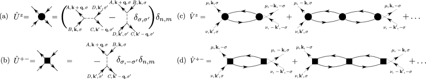
Figure 1: Diagrammatic representations of the matrix elements of (a) $\hat{U}^{z}$ and (b) $\hat{U}^{+-}$. The two lowest-order contributions to the RPA series for the effective pairing interactions for pairs with vanishing total quasi-spin $s_{z}=0$ are shown in (c) for longitudinal particle-hole fluctuations and in (d) for transverse fluctuations. The dotted lines represent the transformation factors $\mathcal{U}$ attached to the external legs.

In this section, we calculate the effective pairing interaction $\Gamma_{\nu,\mu}({\bf k,k^{\prime}})$ in the presence of the SDW but above the SC critical temperature $T_{c}$. The pairing interaction is then inserted into the linearized gap equation,PhysRevLett.17.433 which can be expressed as an eigenvalue problem with the pairing-symmetry functions $\gamma_{\alpha}({\bf k})$ as eigenvectors:

$$-\sum_{j}\oint_{C_{j}}\frac{dk^{\prime}_{\parallel}}{2\pi v_{F}({\bf k^{\prime}})}\;\Gamma_{\nu_{i},\mu_{j}}({\bf k,k^{\prime}})\,\gamma_{\alpha}({\bf k^{\prime}})=\lambda_{\alpha}\,\gamma_{\alpha}({\bf k}).$$ (10)

Herein, $v_{F}({\bf k})=|\nabla_{\bf k}E_{\nu}({\bf k})|$ is the Fermi velocity. The indices $i$ and $j$ label the Fermi pockets and $\nu_{i}$ denotes the band that forms the Fermi pocket with index $i$. The integral is performed along each Fermi pocket; since we work with a two-dimensional model, the Fermi pockets are closed loops $C_{j}$. An eigenvalue $\lambda_{\alpha}\geq 1$ implies that the system is unstable towards a SC phase with gap symmetry given by the corresponding $\gamma_{\alpha}({\bf k})$. We work in the regime $T>T_{c}$, where all eigenvalues are smaller than unity. Nevertheless, the symmetry of the dominant pairing instability is given by the eigenvector to the largest eigenvalue $\lambda_{\rm max}$.

Our calculation of the effective pairing interaction extends the one for the single-band Hubbard model in Ref. PhysRevB.39.11663, . Since we only consider pairing on the Fermi surface and a static SC gap, the interaction is assumed to be frequency independent. We evaluate an infinite RPA-type series of bubble and ladder diagrams. Inter-band pairing, i.e., the formation of Cooper pairs consisting of two electrons from different bands, either involves electrons in states far from the Fermi energy or leads to finite-momentum Cooper pairs, and is therefore excluded. Hence, the Cooper pairs always consist of two electrons from the same band. The summation yields two terms that enter the quartic part of the effective pairing Hamiltonian in addition to the bare interaction:

$$H_{\mathrm{pair}}^{\mathrm{eff}} = -\frac{1}{N}\sum_{\nu,\mu}\sum_{\sigma,\sigma^{\prime}}{\sum_{\bf k,k^{\prime}}}^{\prime}\sum_{i\omega_{n},i\omega_{n}^{\prime}}\sum_{A,B,C,D}\sum_{j,k,n,m}\big{[}\hat{U}^{z}\hat{\chi}^{z}({\bf k-k^{\prime}},i\omega_{n}-i\omega_{n}^{\prime})\,\hat{U}^{z}\big{]}_{(A,B,n,\sigma),(C,D,m,\sigma^{\prime})}$$ (12)

$${}\times{\cal U}^{*}_{A,|j-n|;\nu}({\bf k^{\prime}},\sigma)\,{\cal U}^{*}_{C,|k-m|;\nu}({\bf-k^{\prime}},\sigma^{\prime})\,{\cal U}_{D,k;\mu}({\bf-k},\sigma^{\prime})\,{\cal U}_{B,j;\mu}({\bf k},\sigma)\,d^{\dagger}_{\nu,{\bf k^{\prime}},\sigma}d^{\dagger}_{\nu,{\bf-k^{\prime}},\sigma^{\prime}}d_{\mu,{\bf-k},\sigma^{\prime}}d_{\mu,{\bf k},\sigma}$$

$${}-\frac{1}{N}\sum_{\nu,\mu}\sum_{\sigma,\sigma^{\prime}}{\sum_{\bf k,k^{\prime}}}^{\prime}\sum_{i\omega_{n},i\omega_{n}^{\prime}}\sum_{A,B,C,D}\sum_{j,k,n,m}\big{[}\hat{U}^{+-}\hat{\chi}^{+-}({\bf k-k^{\prime}},i\omega_{n}-i\omega_{n}^{\prime})\,\hat{U}^{+-}\big{]}_{(A,B,n,\sigma),(C,D,m,\sigma^{\prime})}\delta_{\sigma,-\sigma^{\prime}}$$

$${}\times{\cal U}^{*}_{A,|j-n|;\nu}({\bf k^{\prime}},\sigma)\,{\cal U}^{*}_{C,|k-m|;\nu}({\bf-k^{\prime}},\sigma^{\prime})\,{\cal U}_{D,k;\mu}({\bf-k},\sigma)\,{\cal U}_{B,j;\mu}({\bf k},\sigma^{\prime})\,d^{\dagger}_{\nu,{\bf k^{\prime}},\sigma}d^{\dagger}_{\nu,{\bf-k^{\prime}},\sigma^{\prime}}d_{\mu,{\bf-k},\sigma}d_{\mu,{\bf k},\sigma^{\prime}}$$

$${}+\frac{1}{N}\sum_{\nu,\mu}\sum_{\sigma,\sigma^{\prime}}{\sum_{\bf k,k^{\prime}}}^{\prime}\sum_{A,B,C,D}\sum_{j,k,l}U_{(A,B),(C,D)}(\sigma,\sigma^{\prime})$$

$${}\times{\cal U}^{*}_{A,|j-l|;\nu}({\bf k^{\prime}},\sigma)\,{\cal U}^{*}_{C,|k-l|;\nu}({\bf-k^{\prime}},\sigma^{\prime})\,{\cal U}_{D,-k;\alpha}({\bf-k},\sigma^{\prime})\,{\cal U}_{B,j;\mu}({\bf k},\sigma)\,d^{\dagger}_{\nu,{\bf k^{\prime}},\sigma}d^{\dagger}_{\nu,{\bf-k^{\prime}},\sigma^{\prime}}d_{\mu,{\bf-k},\sigma^{\prime}}d_{\mu,{\bf k},\sigma}$$

$$\equiv \frac{1}{N}\sum_{\nu,\mu}\sum_{\sigma,\sigma^{\prime}}{\sum_{\bf k,k^{\prime}}}^{\prime}\sum_{i\omega_{n},i\omega_{n}^{\prime}}V^{z}_{\nu,\mu;\sigma,\sigma^{\prime}}({\bf k,k^{\prime}},i\omega_{n}-i\omega_{n}^{\prime})\,d^{\dagger}_{\nu,{\bf k^{\prime}},\sigma}d^{\dagger}_{\nu,{\bf-k^{\prime}},\sigma^{\prime}}d_{\mu,{\bf-k},\sigma^{\prime}}d_{\mu,{\bf k},\sigma}$$

$${}+\frac{1}{N}\sum_{\nu,\mu}\sum_{\sigma}{\sum_{\bf k,k^{\prime}}}^{\prime}\sum_{i\omega_{n},i\omega_{n}^{\prime}}V^{+-}_{\nu,\mu;\sigma,-\sigma}({\bf k,k^{\prime}},i\omega_{n}-i\omega_{n}^{\prime})\,d^{\dagger}_{\nu,{\bf k^{\prime}},\sigma}d^{\dagger}_{\nu,{\bf-k^{\prime}},-\sigma}d_{\mu,{\bf-k},\sigma}d_{\mu,{\bf k},-\sigma}$$

$${}+\frac{1}{N}\sum_{\nu,\mu}\sum_{\sigma,\sigma^{\prime}}{\sum_{\bf k,k^{\prime}}}^{\prime}V^{0}_{\nu,\mu;\sigma,\sigma^{\prime}}({\bf k,k^{\prime}})\,d^{\dagger}_{\nu,{\bf k^{\prime}},\sigma}d^{\dagger}_{\nu,{\bf-k^{\prime}},\sigma^{\prime}}d_{\mu,{\bf-k},\sigma^{\prime}}d_{\mu,{\bf k},\sigma}.$$

Herein, the RPA susceptibilities take the well-known form

$$\hat{\chi}^{z}({\bf q},iq_{n}) = \hat{\chi}^{z(0)}({\bf q},iq_{n})\big{[}\hat{1}+\hat{U}^{z}\hat{\chi}^{z(0)}({\bf q},iq_{n})\big{]}^{-1},$$ (13)

$$\hat{\chi}^{+-}({\bf q},iq_{n}) = \hat{\chi}^{+-(0)}({\bf q},iq_{n})\big{[}\hat{1}-\hat{U}^{+-}\hat{\chi}^{+-(0)}({\bf q},iq_{n})\big{]}^{-1}.$$

The interaction matrices appearing in the effective interaction have the components

$$U^{z}_{(A,B,n,\sigma),(C,D,m,\sigma^{\prime})} = U_{(A,B),(C,D)}(\sigma,\sigma^{\prime})\,\delta_{n,m}$$

$${}-U_{(A,D),(C,B)}(\sigma,\sigma^{\prime})\,\delta_{n,m}\delta_{\sigma,\sigma^{\prime}},$$

$$U^{+-}_{(A,B,n,\sigma),(C,D,m,\sigma^{\prime})} = U_{(A,D),(C,B)}(\sigma,\sigma^{\prime})\,\delta_{n,m}\delta_{\sigma,-\sigma^{\prime}}.$$

The diagrammatic representation of the two vertices described by these interaction matrices is shown in Figs. 1(a) and 1(b). $\hat{V}^{z}$ and $\hat{V}^{+-}$ can then be understood as two separate series of diagrams that contain either $\hat{U}^{z}$ or $\hat{U}^{+-}$ but are otherwise identical except for the spin indices. The two lowest-order diagrams in these series contributing to pairing with opposite quasi-spins are shown in Figs. 1(c) and 1(d).

The components of the bare susceptibility matrices are given by

$$\chi^{z(0)}_{(A,B,n,\sigma),(C,D,m,\sigma^{\prime})}({\bf q},iq_{n})$$ (17)

$$\equiv\chi^{z(0)}_{(A,B,\sigma),(C,D,\sigma^{\prime})}({\bf q}+n{\bf Q},iq_{n};{\bf q}+m{\bf Q},iq_{n})$$

$$\equiv-\frac{1}{\beta V}{\sum_{{\bf k},i\omega_{n}}}^{\!\!\prime}\sum_{i,j,\nu,\mu}G^{(0)}_{\nu}({\bf k-q},i\omega_{n}-iq_{n})G^{(0)}_{\mu}({\bf k},i\omega_{n})$$

$${}\times{\cal U}^{*}_{A,i;\mu}({\bf k},\sigma)\,{\cal U}_{B,|i-n|;\nu}({\bf k-q},\sigma^{\prime})$$

$${}\times{\cal U}^{*}_{C,|j-m|;\nu}({\bf k-q},\sigma^{\prime})\,{\cal U}_{D,j;\nu}({\bf k},\sigma)\,\delta_{\sigma,\sigma^{\prime}}$$

and

$$\chi^{+-(0)}_{(A,B,n,\sigma),(C,D,m,\sigma^{\prime})}({\bf q},iq_{n})$$ (18)

$$\equiv\chi^{+-(0)}_{(A,B,\sigma),(C,D,\sigma^{\prime})}({\bf q}+n{\bf Q},iq_{n};{\bf q}+m{\bf Q},iq_{n})$$

$$\equiv-\frac{1}{\beta V}{\sum_{{\bf k},i\omega_{n}}}^{\!\!\prime}\sum_{i,j,\nu,\mu}G^{(0)}_{\nu}({\bf k-q},i\omega_{n}-iq_{n})G^{(0)}_{\mu}({\bf k},i\omega_{n})$$

$${}\times{\cal U}^{*}_{A,i;\mu}({\bf k},\sigma)\,{\cal U}_{B,|i-n|;\nu}({\bf k-q},\sigma^{\prime})$$

$${}\times{\cal U}^{*}_{C,|j-m|;\nu}({\bf k-q},\sigma^{\prime})\,{\cal U}_{D,j;\nu}({\bf k},\sigma)\,\delta_{\sigma,-\sigma^{\prime}},$$

where $G^{(0)}_{\nu}({\bf k},i\omega_{n})=(-i\omega_{n}+E_{\nu,{\bf k}})^{-1}$ is the bare electronic Green function in the new basis. The susceptibility $\hat{\chi}^{z(0)}$ describes fluctuations with spin projection $s_{z}=0$ and consists of a longitudinal spin and a charge contribution. $\hat{\chi}^{+-(0)}$ describes transverse spin fluctuations with $s_{z}=\pm 1$. Note that the SDW formation does not mix states with different $s_{z}$ since the z component of spin remains conserved. Thus in this context we do not need to distinguish between spins and quasi-spins.

The superconducting order parameter in the SDW phase is a particle-particle expectation value of the new d quasiparticles, which are connected to the original electrons by the spin-dependent transformation in Eq. (8). As noted above, the quasi-spin of the d quasiparticles is not the same as the spin of the original electrons. Indeed, spin-singlet and spin-triplet states with $s_{z}=0$ are mixed in the SDW phase. This is clearly seen if for example the singlet order parameter in the SDW phase is expressed in terms of the original basis:

$$\langle d_{\nu,{\bf k},\sigma}^{\dagger}d_{\nu,{\bf-k},-\sigma}^{\dagger}-d_{\nu,{\bf k},-\sigma}^{\dagger}d_{\nu,{\bf-k},\sigma}^{\dagger}\rangle$$ (19)

$$=\sum_{A,m}\sum_{B,n}\big{\{}{\cal U}^{*}_{A,m;\nu}({\bf k},\sigma)\,{\cal U}^{*}_{B,n;\nu}({\bf-k},-\sigma)$$

$${}\times\langle c^{\dagger}_{A,{\bf k}+m{\bf Q},\sigma}c^{\dagger}_{B,{\bf-k}+n{\bf Q},-\sigma}\rangle$$

$${}-{\cal U}^{*}_{A,m;\nu}({\bf k},-\sigma)\,{\cal U}^{*}_{B,n;\nu}({\bf-k},\sigma)$$

$${}\times\langle c^{\dagger}_{A,{\bf k}+m{\bf Q},-\sigma}c^{\dagger}_{B,{\bf-k}+n{\bf Q},\sigma}\rangle\big{\}}.$$

We see that an expectation value $\langle d_{\nu,{\bf k},\sigma}^{\dagger}d_{\nu,{\bf-k},-\sigma}^{\dagger}-d_{\nu,{\bf k},-\sigma}^{\dagger}d_{\nu,{\bf-k},\sigma}^{\dagger}\rangle$, which is odd under quasi-spin inversion $\sigma\rightarrow-\sigma$, contains expectation values $\langle c_{A,{\bf k}+m{\bf Q},\sigma}^{\dagger}c_{B,{\bf-k}+n{\bf Q},-\sigma}^{\dagger}+c_{A,{\bf k}+m{\bf Q},-\sigma}^{\dagger}c_{B,{\bf-k}+n{\bf Q},\sigma}^{\dagger}\rangle$ that are even in spin if ${\cal U}^{*}_{A,m;\nu}({\bf k},\sigma)\,{\cal U}^{*}_{B,n;\nu}({\bf-k},-\sigma)\neq{\cal U}^{*}_{A,m;\nu}({\bf k},-\sigma)\,{\cal U}^{*}_{B,n;\nu}({\bf-k},\sigma)$. Analogously, a triplet order parameter can contain expectation values with singlet symmetry in the original basis. However, in the new basis it is still reasonable to distinguish between pairing states that are odd in quasi-spin $\sigma$ and therefore even in ${\bf k}$ and those that are even in $\sigma$ and odd in ${\bf k}$. In the following, we will refer to them as quasi-spin-singlet and quasi-spin-triplet states, respectively.

Since spin-rotation symmetry is broken in the SDW phase, quasi-spin-triplet pairing with $s_{z}=\pm 1$ and with $s_{z}=0$ is not equivalent and the two cases must be considered separately. However, the two triplet states with $|s_{z}|=1$ are still degenerate. (Also recall that $s_{z}=\pm 1$ and $s_{z}=0$ states are not mixed by the SDW formation.)

The pairing interactions in the various SC channels can be constructed from the effective interactions in Eq. (12). Recall that we take the pairing interactions to be frequency independent. Hence, we take the static limit of the susceptibilities in the following. In the static limit, $V^{z}_{\nu,\mu;\sigma,\sigma^{\prime}}$, $V^{+-}_{\nu,\mu;\sigma,\sigma^{\prime}}$, and $V^{0}_{\nu,\mu;\sigma,\sigma^{\prime}}$ are symmetric under interchange of $\sigma$ and $\sigma^{\prime}$. Therefore, we can decompose the pairing interaction, Eq. (12), into a singlet and two triplet channels in the standard manner:Bickers1989206

$$H^{\mathrm{eff}}_{\mathrm{pair}} = \frac{1}{2N}{\sum_{{\bf k,k^{\prime}}}}^{\prime}\sum_{\nu,\mu}\sum_{\sigma}\left\{\left[V^{0}_{\nu,\mu;\sigma,-\sigma}({\bf k,k^{\prime}})+V^{z}_{\nu,\mu;\sigma,-\sigma}({\bf k,k^{\prime}})-V^{+-}_{\nu,\mu;\sigma,-\sigma}({\bf k,k^{\prime}})\right]+[{\bf k}^{\prime}\rightarrow-{\bf k}^{\prime}]\right\}$$ (20)

$${}\times\big{(}d^{\dagger}_{\nu,{\bf k^{\prime}},\sigma}d^{\dagger}_{\nu,{\bf-k^{\prime}},-\sigma}-d^{\dagger}_{\nu,{\bf k^{\prime}},-\sigma}d^{\dagger}_{\nu,{\bf-k^{\prime}},\sigma}\big{)}\big{(}d_{\mu,{\bf-k},-\sigma}d_{\mu,{\bf k},\sigma}-d_{\mu,{\bf-k},\sigma}d_{\mu,{\bf k},-\sigma}\big{)}$$

$${}+\frac{1}{2N}{\sum_{{\bf k,k^{\prime}}}}^{\prime}\sum_{\nu,\mu}\sum_{\sigma}\left\{\left[V^{z}_{\nu,\mu;\sigma,-\sigma}({\bf k,k^{\prime}})+V^{+-}_{\nu,\mu;\sigma,-\sigma}({\bf k,k^{\prime}})\right]-[{\bf k}^{\prime}\rightarrow-{\bf k}^{\prime}]\right\}$$

$${}\times\big{(}d^{\dagger}_{\nu,{\bf k^{\prime}},\sigma}d^{\dagger}_{\nu,{\bf-k^{\prime}},-\sigma}+d^{\dagger}_{\nu,{\bf k^{\prime}},-\sigma}d^{\dagger}_{\nu,{\bf-k^{\prime}},\sigma}\big{)}\big{(}d_{\mu,{\bf-k},-\sigma}d_{\mu,{\bf k},\sigma}+d_{\mu,{\bf-k},\sigma}d_{\mu,{\bf k},-\sigma}\big{)}$$

$${}+\frac{1}{2N}{\sum_{{\bf k,k^{\prime}}}}^{\prime}\sum_{\nu,\mu}\sum_{\sigma}\left\{V^{z}_{\nu,\mu;\sigma,\sigma}({\bf k,k^{\prime}})-[{\bf k}^{\prime}\rightarrow-{\bf k}^{\prime}]\right\}\,d^{\dagger}_{\nu,{\bf k^{\prime}},\sigma}d^{\dagger}_{\nu,{\bf-k^{\prime}},\sigma}d_{\mu,{\bf-k},\sigma}d_{\mu,{\bf k},\sigma}$$

$$\equiv \frac{1}{N}{\sum_{{\bf k,k^{\prime}}}}^{\prime}\sum_{\nu,\mu}\sum_{\sigma}\Gamma^{s}_{\nu,\mu}({\bf k,k^{\prime}})\,\big{(}d^{\dagger}_{\nu,{\bf k^{\prime}},\sigma}d^{\dagger}_{\nu,{\bf-k^{\prime}},-\sigma}-d^{\dagger}_{\nu,{\bf k^{\prime}},-\sigma}d^{\dagger}_{\nu,{\bf-k^{\prime}},\sigma}\big{)}\big{(}d_{\mu,{\bf-k},-\sigma}d_{\mu,{\bf k},\sigma}-d_{\mu,{\bf-k},\sigma}d_{\mu,{\bf k},-\sigma}\big{)}$$

$${}+\frac{1}{N}{\sum_{{\bf k,k^{\prime}}}}^{\prime}\sum_{\nu,\mu}\sum_{\sigma}\Gamma^{t_{0}}_{\nu,\mu}({\bf k,k^{\prime}})\,\big{(}d^{\dagger}_{\nu,{\bf k^{\prime}},\sigma}d^{\dagger}_{\nu,{\bf-k^{\prime}},-\sigma}+d^{\dagger}_{\nu,{\bf k^{\prime}},-\sigma}d^{\dagger}_{\nu,{\bf-k^{\prime}},\sigma}\big{)}\big{(}d_{\mu,{\bf-k},-\sigma}d_{\mu,{\bf k},\sigma}+d_{\mu,{\bf-k},\sigma}d_{\mu,{\bf k},-\sigma}\big{)}$$

$${}+\frac{1}{N}{\sum_{{\bf k,k^{\prime}}}}^{\prime}\sum_{\nu,\mu}\sum_{\sigma}\Gamma^{t_{1}}_{\nu,\mu}({\bf k,k^{\prime}})\,d^{\dagger}_{\nu,{\bf k^{\prime}},\sigma}d^{\dagger}_{\nu,{\bf-k^{\prime}},\sigma}d_{\mu,{\bf-k},\sigma}d_{\mu,{\bf k},\sigma},$$

where $[{\bf k}^{\prime}\rightarrow-{\bf k}^{\prime}]$ represents the preceding terms with $\mathbf{k}^{\prime}$ replaced by $-\mathbf{k}^{\prime}$.

To conclude this section we briefly comment on the relation of our approach to two other methods that are used to obtain effective pairing interactions from repulsive bare interactions. The effective interactions we obtain are closely related to the fluctuation exchange approximation (FLEX).Bickers1989206 In the FLEX, effective two-particle vertices are determined by taking the derivative of a generating functional, which consists of the bare vertices and dressed Green functions, with respect to these Green functions. If only particle-hole processes are considered, this yields expressions for the effective interactions that have the same form as those in Eq. (20), but with the susceptibilities containing the dressed Green functions. In analogy to Ref. 1367-2630-11-2-025016, , our approach can be understood as an additional approximation on top of the FLEX, consisting of replacing dressed Green functions by bare ones. In the paramagnetic limit, our effective interactions recover the form of the FLEX equations for a multiband system given in Ref. PhysRevB.69.104504, , with dressed Green functions replaced by bare ones. Another related method is referred to as perturbative renormalization group (RG). Here, the diagrams that contribute to the effective pairing interaction are only considered up to second order and at temperature $T=0$. The condition that one eigenvalue of the gap equation reaches unity under the RG flow yields an energy scale that is identified with $T_{c}$. This method has been used to study the pairing in various ordered phases of the single-band Hubbard model.PhysRevB.88.064505 It is is exact in the limit of infinitesimal interactions. However, in the pnictides the interaction strengths are of the same order as the band width so that an approximation including higher-order diagrams is desirable.

III Two-band model

To study the effect of an effective pairing interaction mediated by spin and charge fluctuations in a concrete multiband system, we have to specify the band structure and the bare interactions. In the following, we will use a two-band model that captures some important features of many iron pnictides: There is a nearly circular hole pocket in the center of the unfolded BZ and two approximately elliptical electron pockets around $(\pi,0)$ and $(0,\pi)$. We divide the Hamiltonian into noninteracting and interacting components, $H=H_{0}+H_{{\rm int}}$. The noninteracting bands are described by

$$H_{0}=\sum_{\bf k}\sum_{\sigma}\big{(}\epsilon^{c}_{\bf k}c^{\dagger}_{{\bf k}\sigma}c_{{\bf k}\sigma}+\epsilon^{f}_{\bf k}f^{\dagger}_{{\bf k}\sigma}f_{{\bf k}\sigma}\big{)},$$ (21)

where $c^{\dagger}_{{\bf k}\sigma}$ ($f^{\dagger}_{{\bf k}\sigma}$) creates a spin-$\sigma$ electron with momentum ${\bf k}$ in the hole-like (electron-like) band. Neglecting the small orthorhombic distortion, the dispersions arePhysRevB.84.214510 $\epsilon_{{\bf k}}^{c}=\epsilon_{c}+2t_{c}\,(\cos k_{x}a+\cos k_{y}a)-\mu$ and $\epsilon_{{\bf k}}^{f}=\epsilon_{f}+4t_{f}\cos k_{x}a\cos k_{y}a-t_{f}\xi_{e}\,(\cos k_{x}a+\cos k_{y}a)-\mu$, where $a$ is the Fe-Fe bond length and $\mu$ is the chemical potential. In units of $t_{c}$ we set $t_{f}=t_{c}$, $\epsilon_{c}=-3.5t_{c}$, and $\epsilon_{f}=3.0t_{c}$. The parameter $\xi_{e}$ determines the ellipticity of the electron pockets. Here, we choose $\xi_{e}=1$, which corresponds to moderate ellipticity. Figure 2(a) shows the resulting Fermi surface for an electron doping level of $\delta n=0.085$ relative to half filling.

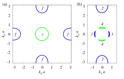
Figure 2: Fermi surface for our model (a) in the paramagnetic phase and (b) in the SDW phase with a SDW gap of $\Delta=0.055t_{c}$ which corresponds to a temperature of $k_{B}T=0.06t_{c}$. The doping has been set to $\delta n=0.085$. In the paramagnetic phase, there is one hole pocket (light green/light gray) and two electron pockets (blue/dark gray). In the SDW phase, there are two hole pockets (light green/light gray) and three electron pockets (blue/dark gray). The letters and numbers specify the bands that form the corresponding Fermi pockets.

Following Ref. PhysRevB.78.134512, , we include four on-site interaction terms in $H_{{\rm int}}$: the intraband Coulomb repulsion, which we set to be equal for both bands,

$$H_{1} = \frac{g_{1}}{V}\sum_{{\bf k,k^{\prime},q}}\big{(}c^{\dagger}_{{\bf k+q}\uparrow}c^{\dagger}_{{\bf k^{\prime}-q}\downarrow}c_{{\bf k^{\prime}}\downarrow}c_{{\bf k}\uparrow}$$ (22)

$${}+f^{\dagger}_{{\bf k+q}\uparrow}f^{\dagger}_{{\bf k^{\prime}-q}\downarrow}f_{{\bf k^{\prime}}\downarrow}f_{{\bf k}\uparrow}\big{)},$$

the interband Coulomb repulsion

$$H_{cf}=\frac{g_{cf}}{V}\sum_{{\bf k,k^{\prime},q}}\sum_{\sigma,\sigma^{\prime}}c^{\dagger}_{{\bf k+q}\sigma}f^{\dagger}_{{\bf k^{\prime}-q}\sigma^{\prime}}f_{{\bf k^{\prime}}\sigma^{\prime}}c_{{\bf k}\sigma},$$ (23)

and two types of correlated interband-hopping transitions,

$$H_{2a} = \frac{g_{2a}}{V}\sum_{{\bf k,k^{\prime},q}}\big{(}c^{\dagger}_{{\bf k+q}\uparrow}c^{\dagger}_{{\bf k^{\prime}-q}\downarrow}f_{{\bf k^{\prime}}\downarrow}f_{{\bf k}\uparrow}+{\rm H.c.}\big{)},$$ (24)

$$H_{2b} = \frac{g_{2b}}{V}\sum_{{\bf k,k^{\prime},q}}\sum_{\sigma,\sigma^{\prime}}c^{\dagger}_{{\bf k+q}\sigma}f^{\dagger}_{{\bf k^{\prime}-q}\sigma^{\prime}}c_{{\bf k^{\prime}}\sigma^{\prime}}f_{{\bf k}\sigma}.$$ (25)

With these interactions, the interaction matrix in Eq. (1) takes the form

$$\hat{U}(\sigma,\sigma^{\prime})$$ (30)

$$=\frac{1}{V}\left(\begin{array}[]{*{4}{c}}g_{1}\delta_{\sigma,-\sigma^{\prime}}&0&0&g_{cf}\\ 0&g_{2a}\delta_{\sigma,-\sigma^{\prime}}&g_{2b}&0\\ 0&g_{2b}&g_{2a}\delta_{\sigma,-\sigma^{\prime}}&0\\ g_{cf}&0&0&g_{1}\delta_{\sigma,-\sigma^{\prime}}\\ \end{array}\right).\quad$$

Only two of the interactions are responsible for the formation of a SDW gap so that a SDW interaction strength $g_{\rm SDW}\equiv g_{cf}+g_{2a}$ can be defined. PhysRevB.24.5713

We have previously shown that this model exhibits a robust SDW phase with ordering vector $\mathbf{Q}=(\pi,0)$ or $(0,\pi)$ for an extended doping range around $\delta n=0.085$.PhysRevB.84.214510 Decoupling within a mean-field approximation, we obtain the Hamiltonian

$$H_{\rm MF} = {\sum_{{\bf k},\sigma}}^{\prime}\left(c^{\dagger}_{{\bf k}\sigma},c^{\dagger}_{{\bf k+Q}\sigma},f^{\dagger}_{{\bf k}\sigma},f^{\dagger}_{{\bf k+Q}\sigma}\right)$$ (39)

$${}\times\left(\begin{array}[]{*{4}{c}}\epsilon_{{\bf k}}^{c}&0&0&\sigma\Delta\\ 0&\epsilon_{{\bf k+Q}}^{c}&\sigma\Delta&0\\ 0&\sigma\Delta&\epsilon_{{\bf k}}^{f}&0\\ \sigma\Delta&0&0&\epsilon_{{\bf k+Q}}^{f}\\ \end{array}\right)\left(\begin{array}[]{*{1}{c}}c_{{\bf k}\sigma}\\ c_{{\bf k+Q}\sigma}\\ f_{{\bf k}\sigma}\\ f_{{\bf k+Q}\sigma}\end{array}\right),\qquad$$

where

$$\Delta=-\frac{g_{\rm SDW}}{2V}\sum_{{\bf k},\sigma}\sigma\,\langle f^{\dagger}_{{\bf k}\sigma}c_{{\bf k+Q}\sigma}\rangle_{\rm MF}$$ (40)

is the mean-field SDW gap and $\langle\ldots\rangle_{\rm MF}$ indicates the thermal average calculated with $H_{\rm MF}$. The mean-field Hamiltonian is diagonalized by a unitary matrix of the form

$$\hat{\cal U}({\bf k},\sigma)=\left(\begin{array}[]{*{4}{c}}-\sigma u_{1,{\bf k}}&0&0&-v_{1,{\bf k}}\\ 0&-\sigma u_{2,{\bf k}}&-v_{2,{\bf k}}&0\\ 0&v_{2,{\bf k}}&-\sigma u_{2,{\bf k}}&0\\ v_{1,{\bf k}}&0&0&-\sigma u_{1,{\bf k}}\\ \end{array}\right),$$ (41)

with the transformation factors

$$u_{1,{\bf k}} = \frac{\epsilon_{fc}^{-}({\bf k})-\sqrt{\epsilon_{fc}^{-}({\bf k})^{2}+\Delta^{2}}}{\sqrt{\Delta^{2}+\left(\epsilon_{fc}^{-}({\bf k})-\sqrt{\epsilon_{fc}^{-}({\bf k})^{2}+\Delta^{2}}\right)^{2}}},$$ (42)

$$v_{1,{\bf k}} = \frac{\Delta}{\sqrt{\Delta^{2}+\left(\epsilon_{fc}^{-}({\bf k})-\sqrt{\epsilon_{fc}^{-}({\bf k})^{2}+\Delta^{2}}\right)^{2}}},$$ (43)

and $u_{2,{\bf k}}=u_{1,{\bf k+Q}}$, $v_{2,{\bf k}}=v_{1,{\bf k+Q}}$. The reconstructed bands are given by

$$E_{1}(\mathbf{k}) = \epsilon_{fc}^{+}(\mathbf{k})+\sqrt{\epsilon_{fc}^{-}(\mathbf{k})^{2}+\Delta^{2}},$$ (44)

$$E_{2}(\mathbf{k}) = \epsilon_{cf}^{+}(\mathbf{k})+\sqrt{\epsilon_{cf}^{-}(\mathbf{k})^{2}+\Delta^{2}},$$ (45)

$$E_{3}(\mathbf{k}) = \epsilon_{cf}^{+}(\mathbf{k})-\sqrt{\epsilon_{cf}^{-}(\mathbf{k})^{2}+\Delta^{2}},$$ (46)

$$E_{4}(\mathbf{k}) = \epsilon_{fc}^{+}(\mathbf{k})-\sqrt{\epsilon_{fc}^{-}(\mathbf{k})^{2}+\Delta^{2}},$$ (47)

where $\epsilon_{ij}^{\pm}({\bf k})=(\epsilon^{i}_{{\bf k+Q}}\pm\epsilon^{j}_{{\bf k}})/2$ and $i$ and $j$ can be $c$ or $f$. The resulting reconstructed Fermi surface is shown in Fig. 2(b). In the SDW phase, the hole Fermi pocket and the electron pocket around $\mathbf{Q}=(\pi,0)$, which is strongly nested with the hole pocket, reconstruct to form four small banana-shaped pockets. Two of these are electron-like and two are hole-like. The electron pocket around $(0,\pi)$ is only weakly affected by the SDW.

IV Analysis of the effective interaction

Even the minimal model introduced above cannot be solved analytically. The matrices $\hat{\chi}^{z}$, $\hat{\chi}^{+-}$, $\hat{\Gamma}^{s}$, $\hat{\Gamma}^{t_{0}}$, and $\hat{\Gamma}^{t_{1}}$ each contain $16\times 16$ components and for non-parabolic bands it is impossible to analytically calculate the susceptibilities appearing in the effective interactions. Nevertheless, it is possible to draw some conclusions about the effective interactions based on analytical considerations, which helps to understand the numerical results presented in Sec. V.

The presence of the Goldstone magnon mode in the SDW phase implies divergent static transverse spin suscpetibilities. Specifically, the components $\chi_{(c,f,1,\uparrow),(c,f,1,\downarrow)}^{+-}$, $\chi_{(c,f,1,\uparrow),(f,c,1,\downarrow)}^{+-}$, $\chi_{(f,c,1,\uparrow),(c,f,1,\downarrow)}^{+-}$, and $\chi_{(f,c,1,\uparrow),(f,c,1,\downarrow)}^{+-}$, and their sum, diverge for ${\bf q}\to 0$ in the magnetic BZ. This begs the question of whether these components lead to a singular contribution to the effective pairing interaction. We first note that this question only pertains to the singlet and $s_{z}=0$ triplet pairing interactions, $\Gamma^{s}({\bf k},{\bf k}^{\prime})$ and $\Gamma^{t_{0}}({\bf k},{\bf k}^{\prime})$ respectively, as only these terms include the contribution $V^{+-}_{\nu,\mu;\sigma,-\sigma}({\bf k-k^{\prime}})$ from the transverse susceptibilities. Furthermore, a possible divergence of these interactions can only occur at ${\bf k}=\pm{\bf k}^{\prime}$. At these points the contribution of the divergent susceptibilities to the interaction is proportional to

$$\sum_{A\neq B}\hbox to0.0pt{$\displaystyle\Big{\{}\big{[}\hat{U}^{+-}\hat{\chi}^{+-}({0})\,\hat{U}^{+-}\big{]}_{(A,B,1,\downarrow),(A,B,1,\uparrow)}$\hss}$$ (48)

$$-\big{[}\hat{U}^{+-}\hat{\chi}^{+-}({0})\,\hat{U}^{+-}\big{]}_{(A,B,1,\downarrow),(B,A,1,\uparrow)}\Big{\}}.$$

For the special case $g_{cf}\neq 0$ and $g_{1}=g_{2a}=g_{2b}=0$, this is in turn proportional to the difference $\chi^{+-}_{(A,B,1,\uparrow),(A,B,1,\downarrow)}(0)-\chi^{+-}_{(A,B,1,\uparrow),(B,A,1,\downarrow)}(0)$, where $A\neq B$. Using the RPA equations (LABEL:chi+-RPA), this difference can be rewritten as

$$\chi^{+-}_{(A,B,1,\uparrow),(A,B,1,\downarrow)}(0)-\chi^{+-}_{(A,B,1,\uparrow),(B,A,1,\downarrow)}(0)$$

$$=\frac{\chi^{+-(0)}_{(A,B,1,\uparrow),(A,B,1,\downarrow)}(0)-\chi^{+-(0)}_{(A,B,1,\uparrow),(B,A,1,\downarrow)}(0)}{1-g_{cf}\big{[}\chi^{+-(0)}_{(A,B,1,\uparrow),(A,B,1,\downarrow)}(0)-\chi^{+-(0)}_{(A,B,1,\uparrow),(B,A,1,\downarrow)}(0)\big{]}}.$$

The denominator of Eq. (LABEL:chi_diff) is non-zero, however, as the individual interband susceptibilities and their sum diverge if

$$\chi^{+-(0)}_{(A,B,1,\uparrow),(B,A,1,\downarrow)}(0)+\chi^{+-(0)}_{(A,B,1,\uparrow),(A,B,1,\downarrow)}(0)=\frac{1}{g_{cf}}.$$ (50)

Since the denominator contains the difference instead of the sum, we hence conclude that the contribution of Eq. (48) to the effective interaction remains finite. We note that a non-vanishing contribution to the interaction does not violate Adler’s theorem, which states that the vertex function describing the coupling of electrons to a Goldstone mode vanishes for zero tranferred momentum,adler ; adlers since a divergence of the magnon propagator compensates for the vanishing vertex function. A similar compensation has been found for the single-band Hubbard model applied to cuprates.PhysRevB.39.11663 ; PhysRevB.46.11884 ; chubukov_pines

In the general case where all of the interaction potentials are allowed to be non-zero, we have found numerically that the pairing interaction remains finite at ${\bf k=k^{\prime}}$ and is a smooth function of the momenta. In Fig. 3, we plot $V^{+-}_{\nu,\mu;\sigma,-\sigma}({\bf k-k^{\prime}})$ for ${\bf k}$ close to ${\bf k}^{\prime}$ and ${\bf k}^{\prime}$ lying on one of the banana-shaped electron pockets for various combinations of the interaction parameters. We see that the effective interaction is indeed a smooth function of momentum. This also justifies dropping the exclusion of the point ${\bf q}={\bf Q}$ from the momentum sums in Sec. II.1.

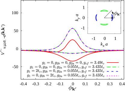
Figure 3: Effective pairing interaction $V^{+-}_{\nu,\mu;\sigma,-\sigma}({\bf k-k^{\prime}})$ around the banana-shaped electron pocket due to transverse spin fluctuations for small ${\bf k}-{\bf k}^{\prime}$ as a function of the polar angle $\phi_{\mathbf{k}^{\prime}}$ of ${\bf k}^{\prime}$ which is shown in the inset. The second momentum ${\bf k}$ is indicated by a black cross. We show two curves for each combination of the bare interaction strengths, one corresponding to the inner and the other to the outer part of the pocket.

V Numerical Results

In this section, we present numerical results for the SC gap structure and its dependence on the interactions $g_{cf}$, $g_{1}$, $g_{2a}$, and $g_{2b}$. For the numerical solution of the mean-field equations for the SDW order parameters $\Delta$, we use a $400\times 400$ k-point mesh in the paramagnetic BZ. The calculation of the bare susceptibilities is performed using a $100\times 100$ k-point mesh. Finally, to solve the SC gap equation (10) we discretize the Fermi surface into 158 points. 128 points of these are chosen on the small banana-shaped Fermi pockets because the calculations are much more sensitive to changes in the number of k-points on these strongly reconstructed pockets. The doping is chosen as $\delta n=0.085$. The SDW interaction is set to $g_{\rm SDW}=3.49t_{c}$, which gives an ordering temperature of $k_{B}T_{N}\approx 0.065t_{c}$ and a reasonable ratio of the zero temperature SDW gap to the band width.PhysRevB.84.214510 The effective pairing interaction is calculated for a temperature of $k_{B}T=0.06t_{c}$.

V.1 Interband Coulomb repulsion $g_{cf}$ and interband hopping $g_{2a}$

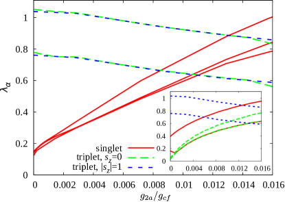
Figure 4: Largest eigenvalues of the linearized gap equation in the singlet and triplet channels, as functions of $g_{2a}/g_{cf}$. We have set $g_{1}=g_{2b}=0$. The inset shows the largest eigenvalues obtained if only longitudinal fluctuations and the bare interaction are considered.

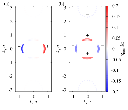
Figure 5: Gap structure of (a) the dominant $s_{z}=0$ triplet state and (b) the dominant singlet state for $g_{2a}/g_{cf}=0.016$. We have set $g_{1}=g_{2b}=0$.

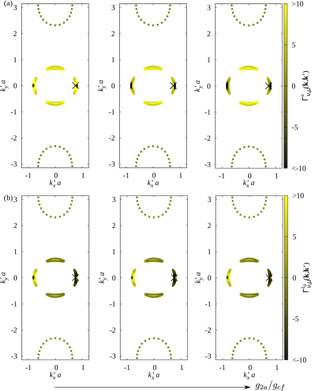
Figure 6: Effective pairing interaction on the Fermi surface as a function of ${\bf k^{\prime}}$. The value of the momentum ${\bf k}$ is indicated by the black cross and the first band index is set to $\nu=1$. From left to right we plot the interaction on the Fermi surface for $g_{2a}/g_{cf}=0$, $g_{2a}/g_{cf}=0.009$, and $g_{2a}/g_{cf}=0.016$ in (a) the singlet channel and (b) the $s_{z}=0$ triplet channel. We have set $g_{1}=g_{2b}=0$.

We first discuss the case where the interactions that do not support a SDW vanish, and so we set $g_{1}=g_{2b}=0$ while fixing the sum of the Coulomb repulsion $g_{cf}$ and the pair-hopping amplitude $g_{2a}$ to be $g_{cf}+g_{2a}=g_{\rm SDW}=3.49t_{c}$. Since a negative value of $g_{2a}$ leads to a charge-density-wave instead of a SDW state,PhysRevB.80.174401 ; PhysRevB.24.5713 we only consider $g_{2a}\geq 0$.

In Fig. 4, we plot the largest eigenvalues obtained from the SC gap equation (10) in the quasi-spin singlet and triplet channels, as functions of the ratio $g_{2a}/g_{cf}$. For very small pair-hopping amplitudes, the triplet pairing dominates. Although the strict degeneracy of the triplet states with $s_{z}=0$ and $s_{z}=1$ is broken, they are nearly degenerate over the complete parameter range and show the same gap structure. The gap structure of the leading triplet state is shown in Fig. 5(a). It has the symmetry of a $p_{x}$-wave state with most of the gap weight on the small electron pockets. Upon increasing the ratio $g_{2a}/g_{cf}$, the eigenvalues belonging to the $s_{z}=0$ triplet states decrease, while the eigenvalues for the singlet states increase. At $g_{2a}/g_{cf}\approx 0.013$, a singlet state becomes the leading SC instability. The gap structure of the leading singlet state is shown in Fig. 5(b); it has the structure of the $s^{\pm}$-type state predicted earlier.PhysRevB.81.174538 ; PhysRevB.82.014521 ; PhysRevB.84.180510 Below $g_{2a}/g_{cf}\approx 0.004$ and above $g_{2a}/g_{cf}\approx 0.016$, the largest eigenvalue exceeds unity. This means that the system becomes unstable towards a SC state. While this formally contradicts the assumption of a normal conducting state made in the derivation, the eigenvector to the largest eigenvalue still gives a good indication of the leading instability. Since the predicted SC critical temperature becomes much higher than experimentally observed values for $g_{2a}/g_{cf}\gtrsim 0.016$, we exclude this parameter range.

The inset in Fig. 4 shows the evolution of the largest eigenvalues as functions of $g_{2a}/g_{cf}$ when the transverse contribution to the interaction is set to zero. In this case the $s_{z}=0$ triplet pairing channel is most strongly reduced while the $s_{z}=1$ triplet is completely unaffected because it originates only from the longitudinal fluctuations. The singlet channel lies in between these extremes. If only the bare interactions are considered the eigenvalues in the triplet channels are strictly zero while the largest eigenvalue in the singlet channel is proportional to $g_{2a}/g_{cf}$ and is reduced by a factor of about $10^{-2}$ compared to the calculation with the full interaction. This shows that the spin and charge fluctuations strongly promote the pairing in the SDW phase.

The crossover from $p_{x}$-wave to $s^{\pm}$-wave pairing can be understood from the evolution of the effective pairing interaction with $g_{2a}/g_{cf}$, which is shown in Fig. 6 as a function of $\mathbf{k}^{\prime}$, for $\mathbf{k}$ lying on the inner part of the right banana-shaped electron pocket. The interaction is peaked at ${\bf k}^{\prime}=\pm{\bf k}$. This peak extends to the other side of the banana-shaped electron pocket, where it takes the opposite sign due to the SDW transformation factors multiplying the susceptibilities. The peak appears in the transverse contribution to the pairing interaction and therefore enters with opposite signs in the singlet and $s_{z}=0$ triplet channels, see Eq. (20). For $g_{2a}/g_{cf}=0$, the peak is strongly negative (positive) and therefore attractive (repulsive) for ${\bf k}^{\prime}\approx{\bf k}$ (${\bf k}^{\prime}\approx-{\bf k}$) in the triplet channel, which supports a sign change of the gap under ${\bf k}\rightarrow-{\bf k}$ and therefore favors a p-wave state. At the same time, the interaction with the other Fermi pockets is weak and thus does not suppress the p-wave state. Upon increasing $g_{2a}/g_{cf}$, the repulsive peak in the singlet interaction at $\mathbf{k}^{\prime}\approx\pm\mathbf{k}$ is suppressed, while the attractive interaction for $\mathbf{k}^{\prime}$ on the other (outer) side of the banana-shaped electron pocket remains strong, see Fig. 6(a). Overall, this leads to a stronger attractive pairing interaction between the two small electron pockets, which favors a singlet state. The repulsion between the small electron and hole pockets then stabilizes a $s^{\pm}$-type structure. In contrast, there is little change in the form of the triplet interaction with increasing $g_{2a}/g_{cf}$, although the strength is overall slightly reduced, see Fig. 6(b).

In Fig. 4, we also plot smaller eigenvalues in each channel. In the $s_{z}=0$ triplet channel, the second largest eigenvalue is clearly separated from the largest eigenvalue and corresponds to a $p_{y}$-wave gap with a line node along the $k_{x}$ axis. In the singlet channel, the three largest eigenvalues are nearly degenerate for $g_{2a}/g_{cf}=0$, but at finite $g_{2a}/g_{cf}\approx 0.004$ they split up. The second and third eigenvalues are nearly degenerate for the interval $0.004\lesssim g_{2a}/g_{cf}\lesssim 0.011$. For larger $g_{2a}/g_{cf}$, the second largest eigenvalue has a $d_{xy}$-type structure with nodes along the $k_{x}$ and $k_{y}$ axes.

V.2 Intraband Coulomb repulsion $g_{1}$

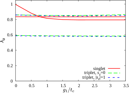
Figure 7: Largest eigenvalues of the linearized gap equation, as functions of the intraband Coulomb interaction $g_{1}$. The ratio of the pair hopping and the interband repulsion has been set to $g_{2a}/g_{cf}=0.016$ with $g_{\rm SDW}=3.49t_{c}$ and $g_{2b}=0$.

We next discuss the intraband Coulomb repulsion with interaction strength $g_{1}$. This term does not affect the SDW order at the mean-field level but can change the SC pairing. We choose the ratio $g_{2a}/g_{cf}=0.016$, for which we have found a $s^{\pm}$-type singlet state as the leading SC instability, and set $g_{2b}=0$. According to Ref. PhysRevB.78.134512, , $g_{1}\approx g_{cf}$ holds if the electron and hole pockets have the same shape. Since we assume weakly elliptical electron pockets we allow for a slightly larger $g_{1}$ and restrict ourselves to the range of $0\leq g_{1}\leq 3.5t_{c}$ in the following.

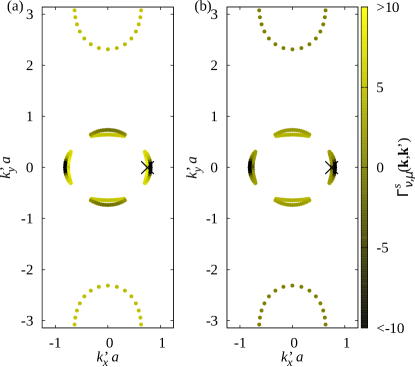
Figure 8: Effective pairing interaction on the Fermi surface in the singlet channel as a function of ${\bf k^{\prime}}$ for (a) $g_{2a}/g_{cf}=0.016$, $g_{1}=2t_{c}$, and $g_{2b}=0$ and (b) $g_{2a}/g_{cf}=0.016$, $g_{1}=0$, and $g_{2b}=2t_{c}$. The value of momentum ${\bf k}$ is indicated by the black cross and the first band index is set to $\nu=1$.

In Fig. 7 we plot the largest eigenvalues from the SC gap equation in the singlet and triplet channels as functions of $g_{1}$. The figure shows that a finite $g_{1}$ leads to the suppression of singlet pairing, while the quasi-spin-triplet states are hardly affected. Consequently, at $g_{1}\approx 0.1t_{c}$ the triplet states become the dominant pairing instabilities again. The gap structure of the dominant triplet state is still the $p_{x}$-wave depicted in Fig. 5(a). The suppression of the singlet state can be understood from the interaction in the singlet channel, which we plot in Fig. 8(a) for $g_{1}=2t_{c}$: The intrapocket interaction is enhanced by the finite $g_{1}$ and the interaction between the electron and the hole pockets becomes less strongly repulsive. Also, the interaction between the small electron pocket and the large electron pocket becomes weakly repulsive. These tendencies disfavor a sign change of the SC gap between electron and hole pockets and hence suppress the eigenvalue corresponding to $s^{\pm}$-type pairing.

The intraband Coulomb repulsion also significantly modifies the dominant singlet pairing state. Already for moderate $g_{1}\approx 0.5t_{c}$, the $s^{\pm}$-type state develops accidental nodes on the small electron pockets, as shown in Fig. 9(a). At $g_{1}\approx 0.7t_{c}$, the two largest eigenvalues in the quasi-spin-singlet channel cross and a state with nodes along the $k_{x}$ and $k_{y}$ axes becomes the dominant singlet state. The gap is plotted in Fig. 9(b). After the crossing, when the $s^{\pm}$-type state is subdominant, it assumes the structure shown in Fig. 9(c). The two largest eigenvalues in the singlet channel remain very close to each other up to $g_{1}=3.5t_{c}$. The appearance of nodes in the gap can be attributed to the increase of the intraband repulsion seen in Fig. 8.

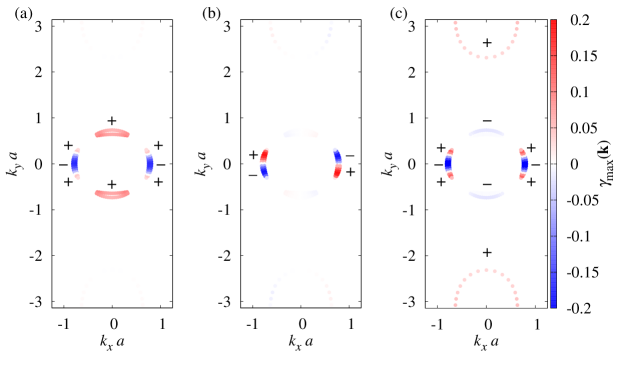
Figure 9: Gap structure of (a) the dominant singlet state for $g_{2a}/g_{cf}=0.013$, $g_{1}=0.77t_{c}$, and $g_{2b}=0$, (b) the dominant singlet state for $g_{2a}/g_{cf}=0.022$, $g_{1}=3.49t_{c}$, and $g_{2b}=0$, and (c) the subdominant singlet state for $g_{2a}/g_{cf}=0.022$, $g_{1}=3.49t_{c}$, and $g_{2b}=0$.

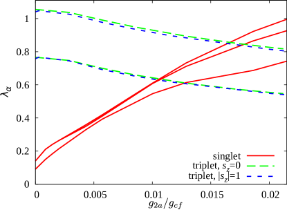
Figure 10: Largest eigenvalues of the linearized gap equation as functions of $g_{2a}/g_{cf}$. The intraband repulsion has been set to $g_{1}=3.49t_{c}$ and $g_{2b}=0$.

Figure 10 shows the evolution of the eigenvalues corresponding to the singlet and triplet channels as functions of $g_{2a}/g_{cf}$ for $g_{1}=3.49t_{c}=g_{\rm SDW}$. It becomes clear that even when the intraband Coulomb repulsion $g_{1}$ takes a rather large value, a small $g_{2a}$ is sufficient to make a quasi-spin-singlet state the dominant SC instability. The leading singlet state then has the structure shown in Fig. 9(b). It is closely followed by a state with the gap depicted in Fig. 9(c), illustrating the tendency of the intraband repulsion to favor nodal gap structures. The close proximity of the eigenvalues for the two different gap structures suggests that small changes in the model, e.g., in the band structure, may change the order of the two eigenvalues.

V.3 Interband-hopping transitions $g_{2b}$

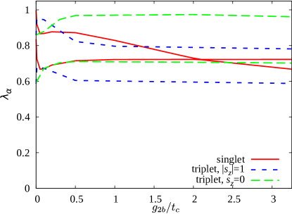
Figure 11: Largest eigenvalues of the linearized gap equation in the singlet and triplet channels, as functions of $g_{2b}$. The ratio of the pair hopping and the interband repulsion has been set to $g_{2a}/g_{cf}=0.013$ with $g_{\rm SDW}=3.49t_{c}$ and $g_{1}=0$.

Finally, we study the effect of the second type of correlated interband-hopping transition with coupling constant $g_{2b}$, given in Eq. (25). We take $g_{2a}/g_{cf}=0.013$ as in Sec. V.2, set $g_{1}=0$, and vary $g_{2b}$. As with the correlated pair hopping $g_{2a}$, the SDW order is only stable for non-negative values of $g_{2b}$. PhysRevB.24.5713 ; PhysRevB.80.174401 Furthermore, it has been pointed out that for the iron pnictides the inequality $g_{2b}<g_{cf}$ is most likely satisfied.PhysRevB.78.134512 Therefore, we only consider the interval $0\leq g_{2b}<g_{cf}=3.445t_{c}$.

In Fig. 11 we plot the largest eigenvalues from the SC gap equation in the singlet and triplet channels as functions of $g_{2b}$. This shows that a finite $g_{2b}$ breaks the near degeneracy of the triplet states with $s_{z}=0$ and $|s_{z}|=1$. We also find that a non-zero $g_{2b}$ leads to a strong suppression of the $s^{\pm}$-type state: Almost immediately upon switching on $g_{2b}$, the $p_{x}$-wave state becomes the dominant SC state again. Similarly to the effect of the intraband repulsion $g_{1}$, we see from Fig. 8(b) that $g_{2b}>0$ leads to a reduction of the repulsion between the small electron and hole pockets, hence reducing the tendency towards a sign change between these pockets and therefore suppressing the $s^{\pm}$-type pairing. At $g_{2b}\approx 2.1t_{c}$, the two largest eigenvalues in the singlet channel cross and a state with the structure shown in Fig. 9(b) becomes the dominant singlet state again.

VI Summary and Conclusions

We have presented a method that allows us to derive an effective pairing interaction for a multiband system in a symmetry-broken SDW phase. Our approach is to decouple an interacting multiband system with general two-particle interactions in the spin channel and to apply a saddle-point approximation to describe the SDW phase. The remaining fluctuations in the decoupling field are integrated out to obtain the quasiparticle interactions in the ordered phase. In the presence of the SDW, we calculate the susceptibilities for transverse and longitudinal particle-hole excitations within the RPA. These susceptibilities determine the effective pairing interaction in the quasi-spin-singlet and quasi-spin-triplet channels. The pairing interactions are then inserted into the linearized gap equation in order to find the leading SC instability. This approach allows us to study the effect of spin and charge fluctuations on the pairing in the SDW phase. In particular, it is an unbiased tool for finding the gap structure of the leading SC instability since the gap structure is obtained as an eigenvector from the gap equation. In this respect our approach is advantageous compared to Ginzburg-Landau calculations that only allow for a limited number of different gap structures.

We have applied this approach to a two-band minimal model for iron pnictides. The effective pairing interaction has been calculated for various combinations of four symmetry-allowed types of interactions: interband and intraband Coulomb repulsion and two types of correlated interband-hopping terms. Our results show that there is a complex interplay between the bare interactions, the susceptibilities, and the transformation factors that arise from the folding of the BZ in the SDW phase. The description of this interplay is the key difference of our approach compared to previous microscopic approaches to describe the coexistence region in the pnictide phase diagram. The effect of the electron-electron interactions on the pairing is not included in a spin-fermion model.0953-8984-23-9-094203 Decoupling the bare interaction within a mean-field approximationPhysRevB.80.100508 ; PhysRevB.83.224513 ; PhysRevB.81.174538 neglects the crucial role of fluctuations in promoting the pairing.

Note that although the interband components of the transverse spin susceptibility diverge, the magnons do not lead to a divergence in the effective pairing interaction. The fluctuation-enhanced interaction leads to the appearance of a quasi-spin-triplet $p_{x}$-wave pairing state that is not found if only the bare interactions are considered. The $p_{x}$-wave state competes with the quasi-spin singlet states, which are much more sensitive to the strengths of the bare interactions. In particular, a finite pair-hopping amplitude $g_{2a}$ is crucial for the formation of singlet pairs, and the singlet eigenvalues react sensitively to changes in the ratio $g_{2a}/g_{cf}$. We expect that this competition can be found also in the spin-fermion model proposed by Wu and Phillips0953-8984-23-9-094203 because the key features of the spin susceptibility are present in both models. However, unlike the itinerant picture, the spin-fermion model is based on the assumption of localized spins. Hence, the physical basis of the two models is quite different and there is no direct mapping between the interaction strengths in our Hamiltonian and the parameters of the spin-fermion model.

Although $g_{1}$ and $g_{2b}$ suppress the singlet pairing, the parameter range in which a triplet state is the dominant instability is limited, as a small increase in $g_{2a}/g_{cf}$ always leads to a dominant singlet state. For $g_{1}=g_{2b}=0$ and $g_{2a}/g_{cf}\gtrsim 0.005$, the singlet channel is clearly dominated by a nodeless $s^{\pm}$-type state suggested to be the most likely pairing state in earlier works.PhysRevB.81.174538 ; PhysRevB.82.014521 ; PhysRevB.84.180510 However, if either $g_{1}$ or $g_{2b}$ are sufficiently large, nodal gap structures are favored. The dominant state for large $g_{1}$ or $g_{2b}$ has nodes along the $k_{x}$ and $k_{y}$ axes.

In conclusion, we find that a nodeless $s^{\pm}$-type singlet pairing state, several nodal singlet states, and a $p_{x}$-wave triplet state can be the leading SC instability in the SDW phase of a two-band model for the iron pnictides. The dominant instability depends sensitively on the four coupling strengths. Hence, these coupling strengths could be constrained by the experimental determination of the gap structure in the coexistence region, which has hitherto not been studied in much detail. Although there are reports of a transition from a nodal to a nodeless state in $\mathrm{Ba}_{1-x}\mathrm{K}_{x}\mathrm{Fe_{2}As_{2}}$ with decreasing hole doping based on thermal-conductivity measurements,arXiv:1105.2232 it is unclear where these nodes appear on the Fermi surface. Momentum-resolved measurements of the gap to distingusih between the different structures are therefore highly desirable, with angle-resolved photoemission spectroscopy (ARPES) being the method of choice. The transition from a nodal to a nodeless structure was explained by Maiti et al.PhysRevB.85.144527 as a result of the change in the SDW gap size with doping. Our work suggests an alternative explanation: we find that the gap structure depends strongly on details of the interactions. In view of our results it is intriguing that the nodes appear when the hole concentration is reduced.arXiv:1105.2232 A reduction of the hole concentration is expected to increase the effective Coulomb repulsion in our Hubbard-type model due to weaker screening. This should result in an increase of the intraband Coulomb repulsion $g_{1}$ relative to the SDW interaction $g_{\rm SDW}$, which we find to stabilize nodal singlet states.

References

- (1) D. C. Johnston, Adv. Phys. 59, 803 (2010).
- (2) P. J. Hirschfeld, M. M. Korshuvnov, and I. I. Mazin, Rep. Prog. Phys. 74, 124508 (2011).
- (3) M. D. Lumsden and A. D. Christianson, J. Phys.: Condens. Matter 22, 203203 (2010).
- (4) H. Luetkens, H.-H. Klauss, M. Kraken, F. J. Litterst, T. Dellmann, R. Klingeler, C. Hess, R. Khasanov, A. Amato, C. Baines, M. Kosmala, O. J. Schumann, M. Braden, J. Hamann-Borrero, N. Leps, A. Kondrat, G. Behr, J. Werner, and B. Büchner, Nature Mat. 8, 305 (2009).
- (5) D. K. Pratt, W. Tian, A. Kreyssig, J. L. Zarestky, S. Nandi, N. Ni, S. L. Bud’ko, P. C. Canfield, A. I. Godman, and R. J. McQueeney, Phys. Rev. Lett. 103, 087001 (2009).
- (6) E. Wiesenmayer, H. Luetkens, G. Pascua, R. Khasanov, A. Amato, H. Potts, B. Banusch, H.-H. Klauss, and D. Johrendt, Phys. Rev. Lett. 107, 237001 (2011).
- (7) S. Avci, O. Chmaissem, E. A. Gremychkin, S. Rosenkranz, J.-P. Castellan, D. Y. Chng, I. S. Todorov, J. A. Schluedter, H. Claus, M. G. Kanatzidis, A. Daoud-Aladine, D. Khalyavin, and R. Osborn, Phys. Rev. B 83, 172503 (2011).
- (8) T. Goko, A. A. Aczel, E. Baggio-Saitovitch, S. L. Bud’ko, P. C. Canfield, J. P. Carlo, G. F. Chen, P. Dai, A. C. Hamann, W. Z. Hu, H. Kageyama, G. M. Luke, J. L. Luo, B. Nachumi, N. Ni, D. Reznik, D. R. Sanchez-Candela, A. T. Savici, K. J. Sikes, N. L. Wang, C. R. Wibe, T. J. Williams, T. Yamamoto, W. Yu, and Y. J. Uemura, Phys. Rev. B 80, 024508 (2009).
- (9) M. S. Tokikachvili, S. L. Bud’ko, N. Ni, and P. C. Canfield, Phys. Rev. Lett. 101, 057006 (2008).
- (10) S. Graser, T. A. Maier, P. J. Hirschfeld, and D. J. Scalapino, New J. Phys. 11, 025016 (2009).
- (11) K. Kuroki, H. Usui, S. Onari, R. Arita, and H. Aoki, Phys. Rev. B 79, 224511 (2009).
- (12) S. Graser, A. F. Kemper, T. A. Maier, H.-P. Cheng, P. J. Hirschfeld, and D. J. Schalapino, Phys. Rev. B 81, 214503 (2010).
- (13) H. Ikeda, R. Arita, and J. Kuneš, Phys. Rev. B 81, 054502 (2010).
- (14) T. Saito, S. Onari, and H. Kontani, Phys. Rev. B 88, 045115 (2013).
- (15) H. Kontani and S. Onari, Phys. Rev. Lett. 104, 157001 (2010).
- (16) T. Saito, S. Onari, and H. Kontani, Phys. Rev. B 82, 144510 (2010).
- (17) H. Ikeda, R. Arita, and J. Kuneš, Phys. Rev. B 82, 024508 (2010).
- (18) R. Khasanov, S. Sanna, G. Prando, Z. Shermadini, M. Bendele, A. Amato, P. Carretta, R. De Renzi, J. Karpinski, S. Katrych, H. Luetkens, and N. D. Zhigadlo, Phys. Rev. B 84, 100501 (2011).
- (19) R. M. Fernandes, D. K. Pratt, W. Tian, J. Zarestky, A. Kreyssig, S. Nandi, M. G. Kim, A. Thaler, N. Ni, P. C. Canfield, R. J. McQueeney, J. Schmalian, and A. I. Goldman, Phys. Rev. B 81, 140501 (2010).
- (20) M.-H. Julien, H. Mayaffre, M. Horvati, C. Berthier, X. D. Zhang, W. Wu, G. F. Chen, N. L. Wang, and J. L. Luo, Europhys. Lett. 87, 37001 (2009).
- (21) Z. Li, R. Zhou, Y. Liu, D. L. Sun, J. Yang, C. T. Lin, and G.-Q. Zheng, Phys. Rev. B 86, 180501 (2012).
- (22) R. M. Fernandes and J. Schmalian, Phys. Rev. B 82, 014521 (2010).
- (23) A. B. Vorontsov, M. G. Vavilov, and A. V. Chubukov, Phys. Rev. B 81, 174538 (2010).
- (24) D. Parker, M. G. Vavilov, A. V. Chubukov, and I. I. Mazin, Phys. Rev. B 80, 100508(R) (2009).
- (25) P. Ghaemi and A. Vishwanath, Phys. Rev. B 83, 224513 (2011).
- (26) S. Maiti, R. M. Fernandes, and A. V. Chubukov, Phys. Rev. B 85, 144527 (2012).
- (27) J.-P. Reid, M. A. Tantatar, X. G. Luo, H. Shakeripour, S. Ren de Cotret, N. Doiron-Leyraud, J. Chang, B. Shen, H.-H. Wen, H. Kim, R. Prozorov, and L. Taillefer, arXiv:1105.2232v1 (2011).
- (28) J. Wu and P. Phillips, J. Phys.: Condens. Matter 23, 094203 (2011).
- (29) N. F. Berk and J. R. Schrieffer, Phys. Rev. Lett. 17, 433 (1966).
- (30) J. R. Schrieffer, X. G. Wen, and S. C. Zhang, Phys. Rev. B 39, 11663 (1989).
- (31) A. V. Chubukov and D. M. Frenkel, Phys. Rev. B 46, 11884 (1992).
- (32) A. V. Chubukov, D. V. Efremov, and I. Eremin, Phys. Rev. B 78, 134512 (2008).
- (33) P. M. R. Brydon and C. Timm, Phys. Rev. B 84, 174401 (2009).
- (34) J. Knolle, I. Eremin, J. Schmalian, and R. Moessner, Phys. Rev. B 84, 180510 (2011).
- (35) P. M. R. Brydon, J. Schmiedt, and C. Timm, Phys. Rev. B 84, 214510 (2011).
- (36) N. Bickers and D. J. Scalapino, Ann. Phys. 193, 206 (1989).
- (37) T. Takimoto, T. Hota, and K. Ueda, Phys. Rev. B 69, 104504 (2004).
- (38) W. Cho, R. Thomale, S. Raghu, and S. A. Kivelson, Phys. Rev. B 88, 064505 (2013).
- (39) D. W. Buker, Phys. Rev. B 24, 5713 (1981).
- (40) S. L. Adler, Phys. Rev. 137, B1022 (1965).
- (41) A. Bourque, C. Gale, and K. L. Haglin, Int. J. Mod. Phys. A 20, 6169 (2005).
- (42) A. V. Chubukov, D. Pines, and J. Schmalian, in The Physics of Conventional and Unconventional Superconductors, edited by K. H. Bennemann and J. B. Ketterson (Springer, Berlin, 2002).
- (43) J.-P. Ismer, I. Eremin, E. Rossi, D. K. Morr, and G. Blumberg, Phys. Rev. Lett. 105, 037003 (2010).