Set-valued solutions for non-ideal detonation

Abstract

The existence and structure of steady gaseous detonation propagating in a packed bed of solid inert particles are analyzed in the one-dimensional approximation by taking into consideration frictional and heat losses between the gas and the particles. A new formulation of the governing equations is introduced that eliminates the well-known difficulties with numerical integration across the sonic singularity in the reactive Euler equations. The new algorithm allows us to determine that the detonation solutions as the loss factors are varied have a set-valued nature at low detonation velocities when the sonic constraint disappears from the solutions. These set-valued solutions correspond to a continuous spectrum of the eigenvalue problem that determines the velocity of the detonation.

1 Introduction

Detonation is a shock wave in a reactive medium that is sustained by the energy released in the chemical reactions initiated by the passage of the wave. Gaseous detonation propagating in a tube, in the interstitial space in a porous medium, or other obstructed environments is subject to resistance due to heat transfer, boundary layers and shock reflections that arise at the interfaces between the gas and the obstacles or the walls of the tube. Such resistance leads to momentum and energy losses in the gas that can significantly affect the propagation of the detonation. In the presence of such losses, the detonation is termed “non-ideal”, and its propagation velocity is lower than in the case (termed “ideal”) when there are no such losses. This drop in the detonation velocity is called the “velocity deficit”. Quantifying the velocity deficit in terms of the losses is one of the major problems in detonation theory and its study goes back to the original paper by Zel’dovich [18] (see also the classic book by Zel’dovich and Kompaneets [21]). An important feature observed in experiments on non-ideal detonation waves is their ability to propagate with velocities ranging from near sonic speed in the ambient gas, $c_{a}$, to the ideal Chapman-Jouguet (CJ) value, $D_{\mathrm{CJ}}$ [12, 14, 15, 13]. The physical mechanisms responsible for this self-sustained propagation of detonation depend on the extent and the nature of the losses. A particularly interesting aspect is the possibility that the frictional heating of the gas dominates over its heating by chemical reactions at low detonation velocities. We also mention a peculiar theoretical observation, first discussed in [18], that in the presence of losses, the flow in the detonation reaction zone can reverse its direction; that is, the velocity can become negative in the laboratory frame of reference, a situation typical for flames, but unusual for detonations. No experimental evidence for this prediction appears to exist.

Since the early works mentioned above, this problem has been revisited many times by researchers seeking to understand the precise mechanisms of detonation propagation when the effects of losses are substantial. A particularly important issue, from a practical point of view, is the existence of detonation limits. The limit of detonation propagation is defined as a threshold in terms of some control quantity (e.g., a tube diameter) below which the detonation cannot propagate. The problem of defining such limits is nontrivial and is complicated by the fact that detonation can and most often does propagate unsteadily. Although this fact makes the definitions of these limits based on the non-existence of stationary solutions somewhat limited in application, understanding the steady-state solutions is a major first step in understanding the nature of detonation limits as well as in building a theory of unsteady detonations.

Theoretical work on the role of losses in detonations was continued in [20, 19, 2, 3]. In [20], both convective and conductive heat losses were considered. Convective losses depend on the relative velocity between the gas and the particles/walls and they vanish as the relative velocity vanishes. In contrast, conductive losses persist in the absence of the relative velocity. In the relaxation zone far downstream of the lead shock, where the flow of the reaction products has sufficiently decelerated, the authors of [20] assumed that the heat losses corresponded to an approximately constant Nusselt number and thus were of the conductive type. Subsequently, they reasoned that the gas in the products cooled down due to the conductive heat transfer and reached a state of rest far downstream but with the same pressure and density as the upstream state with the fresh mixture.

In contrast, the model we present here involves only convective heat losses, as a consequence of which the heat transfer from the gas to the particles vanishes when the gas stops. This is a reasonable assumption for detonations because the conductive losses occur on time scales that are much longer than the time scale of the detonation propagation. The temperature relaxation in the products can therefore not be expected to affect the detonation dynamics over the time scales of interest. We should note that our governing equations take the same general form as those in [18, 21, 20] and include the momentum loss due to friction, heat loss, which is proportional to the temperature difference between the gas and the solid particles, and the effect of heating of the gas due to the friction.

Convective heat transfer was also considered in [3]. The heat loss term in the energy equation in [3] is slightly different from that of [18, 21, 20] and hence also different from our model. In addition and more importantly, the far-field conditions in [3] include a prescribed temperature value. This prescribed condition on the product temperature follows directly from the energy equation when the heat losses are neglected [2]. However, in the presence of heat losses, imposing a prescribed temperature of the products is difficult to justify. The only condition that we impose here is that of the vanishing velocity in the products. The product temperature is therefore an outcome of the solution of the steady-state equations, not something prescribed. As a result, this formulation has an interesting consequence: a new class of solutions with a continuous spectrum of detonation velocities arises.

To highlight the most important general features of detonation in systems with losses that have been found previously, we mention that, in qualitative agreement with prior experimental research [12, 14, 15, 13], different regimes of detonation propagation have been theoretically identified in [2, 3]:

1) When the detonation speed is below the ideal CJ value but not substantially, the wave has a structure that is very similar to that of the classical ZND theory (Zel’dovich [18], von Neumann [16] and Döring [5]; see also [9]) of a self-sustained detonation with its inherent transonic character in the post-shock flow and with a sonic point located at some distance from the shock.

2) When the detonation speed drops significantly, often to around $0.6$ of the ideal value, the sonic locus moves to infinity and, with a further decrease of the detonation velocity, disappears from the flow altogether. This structure, in which the post-shock flow is entirely subsonic in the shock-fixed frame, resembles piston-supported overdriven detonations. However, the latter gain energy from the piston and therefore propagate faster than CJ detonations. In contrast, non-ideal detonation, with a subsonic post-shock flow, has no support and propagates at velocities that are substantially lower than the ideal CJ velocity. Because its structure is missing a sonic point, it is not a self-sustained wave.

In experiments, the velocity deficits are obtained by, for example, decreasing the initial pressure, $p_{a}$, in the explosive mixture [12, 14, 15, 13]. In many cases, a decrease in $p_{a}$ to some critical value results in an abrupt decrease in the speed to subsonic velocities, which is more closely associated with turbulent deflagration waves than with detonations. In theoretical modeling, one can, in principle, look at the solutions that have even smaller velocity than the ambient sound speed, as was done in [2, 3] and in subsequent works by the same authors and their collaborators. However, in such cases, the structure does not contain a shock and the wave is subsonic relative to the state upstream. We limit the discussion in this work to supersonic waves containing a shock as an inherent element of the structure.

While the nature of self-sustained non-ideal detonation is relatively clear, that of the regime with subsonic post-shock flow has led to some conflicting conclusions in the literature. In particular, the existence of steady solutions of the governing equations in this regime was questioned in [4]. Indeed, because the sonic point disappears from the flow, the classical self-sustained structure cannot be a solution. It therefore appears reasonable to conclude that no steady-state solutions exist in this case. In [2, 3], however, the authors have been able to construct the steady $D$-$c_{f}$ relations in the entire range of velocities from the ideal $D=D_{\mathrm{CJ}}$ value to the sonic velocity, $D=c_{a}$ (and even further below), where $c_{a}$ is the speed of sound in the upstream mixture and $c_{f}$ is the dimensionless drag coefficient. Instead of the sonic conditions, they applied $u=0$ at infinity and solved the appropriate boundary value problem. In this connection, a point that requires certain care in interpretation is the question of the existence of a steady-state solution versus its stability. Numerical simulations in [4, 6] indicate that detonation with frictional momentum losses is unstable; in fact, it is more unstable in the presence of losses than in their absence. Because of the instability, the steady-state solutions cannot be reached as long-time asymptotic solutions of an initial value problem of the underlying reactive Euler equations. This, however, does not imply that the steady-state solutions of the equations do not exist. In order to establish the existence of the steady-state solutions, we must be able to solve the appropriate boundary value problem for the time-independent governing equations. Importantly, the proper statement of such a boundary value problem does not necessarily involve sonic conditions. We discuss this point in detail in the subsequent sections of this paper.

In this work, we show that the steady-state solutions of the governing reactive Euler equations with heat and momentum losses have a peculiar nature in that the $D$-$c_{f}$ dependence is no longer a curve, but rather a set-valued function. When the sonic locus disappears from the flow, at a given loss coefficient, there exists a continuous range of detonation velocities, all corresponding to steady-state solutions of the governing equations. Effectively, $D$, as the eigenvalue of the nonlinear eigenvalue problem, is found to have both discrete and continuous spectra. This is in contrast with prior results, in which either the steady-state solution appears not to exist [4] or that there is a Z-shaped curve in the $D$-$c_{f}$ plane, giving a finite and discrete set of solutions for a given $c_{f}$ [11].

Another contribution of our work is a new formulation of the governing equations that completely avoids the difficulty of integrating through the sonic locus. The latter is a well-recognized problem in detonation theory [20, 11, 1]. We have discovered a new set of dependent variables in which the governing equations are no longer singular at the sonic point. This finding results in a numerically well-conditioned integration of the detonation structure in the entire flow region. Generalization of the algorithm to incorporate other loss factors and multiple reactions is possible and is introduced in [8].

A possibility of flow reversal in the reaction zone [18] was also briefly discussed in [20], where the authors continued the analysis of the problem and found that, with the far-field conditions they used, the convective heat transfer between the gas and the tube walls (or solid particles) was insufficient to cause the flow reversal. However, with the inclusion of conductive heat losses, flow reversal was indeed found. The authors of [3] did not discuss this possibility even though convective heat transfer was also an essential element of their analysis. Our present finding is that, with convective heat transfer, flow reversal necessarily occurs in the regime where the flow behind the shock is entirely subsonic. In contrast, no flow reversal is possible with only friction losses. We emphasize, however, that our far-field conditions are different from those of [20] and [3].

The remainder of this paper is organized as follows. In Section 2, we introduce reactive Euler equations that are subject to the momentum and heat exchange terms. The Rankine-Hugoniot conditions are also introduced in this section. In Section 3, we discuss the steady-state solutions and introduce a change of dependent variables that removes the sonic singularities from the equations. In Section 4, we calculate various solutions when both the friction and heat loss terms are present and show that the detonation speed versus loss coefficient is a set-valued function. Concluding remarks are offered in Section 5.

2 Governing equations

Consider a detonation in a perfect gas that fills the interstitial space in a packed bed of solid particles of diameter $d$. The particles are assumed to be immobile and inert; their only role is to exchange momentum and energy with the detonating gas. The chemical reaction in the gas is described globally as $Reactant\to Product$. The progress of this reaction is measured by variable, $\lambda$, that goes from $0$ at the shock to $1$ in the fully burnt gas. The reaction rate is assumed to be given in the Arrhenius form,

$$\omega=k\left(1-\lambda\right)\exp\left(-\frac{E}{pv}\right),$$ (1)

where $E$ is the activation energy, $p$ is the pressure, and $v$ is the specific volume. The perfect-gas equation of state is assumed to be given by

$$e_{i}=\frac{pv}{\gamma-1},$$ (2)

where $\gamma$ is the constant ratio of specific heats.

With these modeling assumptions, the governing reactive Euler equations further incorporating the heat and momentum exchange between the gas and particles are as follows. The continuity equation is

$$\rho_{t}+(\rho u)_{x}=0,$$ (3)

where $\rho=1/v$ and $u$ are the gas density and velocity, respectively. The gas momentum equation is

$$u_{t}+uu_{x}=-\frac{1}{\rho}p_{x}-\frac{f}{\rho\phi},$$ (4)

or in conservation form,

$$\left(\rho u\right)_{t}+\left(p+\rho u^{2}\right)_{x}=-\frac{f}{\phi},$$ (5)

where the drag force due to the solid particles is assumed to take the form [10],

$$f=A_{s}\rho\left(b_{1}+\frac{b_{2}}{Re}\right)u|u|,$$ (6)

with

$$A_{s}=\frac{4\phi}{d_{p}},\quad d_{p}=\frac{2\phi d}{3(1-\phi)},\quad\mathrm{Re}=\frac{d_{p}|u|}{\nu},$$ (7)

where $\phi$ is the porosity of the packed bed, i.e., the fraction of space occupied by the gas, $d$ is the particle diameter, $\mathrm{Re}$ is the Reynolds number, $\nu$ is the gas kinematic viscosity, $b_{1}$ and $b_{2}$ are numerical constants. In the calculations below, we take $\phi=0.4$, $b_{1}=0.75$, $b_{2}=0$ [10], thereby assuming high Reynolds number friction losses.

The energy equation can be written as

$$p_{t}+up_{x}+\gamma pu_{x}=\left(\gamma-1\right)Q\rho\omega+\left(\gamma-1\right)\left(\frac{uf-h}{\phi}\right).$$ (8)

It contains contributions due to: 1) the chemical energy release (the first term, wherein $Q$ is the heat release), 2) the work done by the friction forces (the second term, involving $uf$), and 3) the heat transfer between the gas and particles (the last term, involving $h$). The heat exchange rate, $h$, is given by Newton’s law,

$$h=A_{s}\alpha_{s}\left(T-T_{s}\right),$$ (9)

in which the particle temperature is denoted by $T_{s}$ and the heat conduction coefficient, $\alpha_{s}$, is calculated from [10]

$$\alpha_{s}=\lambda_{g}\frac{\mathrm{Nu}}{d_{p}},$$ (10)

where $\mathrm{Nu}=a_{1}+a_{2}\mathrm{Re}^{m}$ is the Nusselt number, $\lambda_{g}$ is the heat conductivity of the gas, and $a_{1}$, $a_{2}$, $m$ are numerical constants. We take $a_{1}=0$, $a_{2}=0.0425$ and $m=1$ [10], thereby assuming purely convective losses. The validity of this approximation for heat transfer in flows in packed beds of solid particles is justified in [10].

In conservation form, the energy equation becomes

$$\left(\rho e\right)_{t}+\left(\rho u\left(e+pv\right)\right)_{x}=-\frac{h}{\phi},$$ (11)

where

$$e=e_{i}+\frac{u^{2}}{2}-\lambda Q=\frac{pv}{\gamma-1}+\frac{u^{2}}{2}-\lambda Q.$$ (12)

The reaction rate equation is

$$\lambda_{t}+u\lambda_{x}=\omega,$$ (13)

or in conservation form,

$$\left(\rho\lambda\right)_{t}+\left(\rho u\lambda\right)_{x}=\rho\omega.$$ (14)

We note that these equations with appropriate modifications of the loss terms can also be used to describe gaseous detonation in rough tubes. The ideas that follow are expected to carry over to such a setting without significant changes.

Across the shock-discontinuity surface, the following Rankine-Hugoniot conditions hold:

$$-D[\rho]+[\rho u]=0,$$ (15)

$$-D[\rho u]+[p+\rho u^{2}]=0,$$ (16)

$$-D[\rho e]+[\rho u(e+pv)]=0,$$ (17)

$$-D[\rho\lambda]+[\rho u\lambda]=0.$$ (18)

Here $U_{a}=\left(\rho_{a},\,u_{a},\,p_{a},\,\lambda_{a}\right)$ is the ambient state ahead of the shock, $U_{s}=\left(\rho_{s},\,u_{s},\,p_{s},\,\lambda_{s}\right)$ is the state immediately after the shock and $[j]=j_{a}-j_{s}$ denotes a jump of $j$ across the shock. For a perfect gas, the shock conditions can be solved explicitly and the following expressions give the post-shock state in terms of the upstream state,

$$\frac{p_{s}}{p_{a}}=\frac{2\gamma}{\gamma+1}M_{a}^{2}-\frac{\gamma-1}{\gamma+1},$$ (19)

$$\frac{u_{s}}{c_{a}}=\frac{2}{\gamma+1}\frac{M_{a}^{2}-1}{M_{a}},$$ (20)

$$\frac{\rho_{s}}{\rho_{a}}=\frac{\left(\gamma+1\right)M_{a}^{2}}{2+\left(\gamma-1\right)M_{a}^{2}},$$ (21)

$$\lambda_{s}=0.$$ (22)

Here $M_{a}=D/c_{a}$ is the detonation Mach number with respect to the upstream state.

3 Steady-state solutions

In this section, we analyze the existence of the steady-state solutions of the governing equations and calculate their properties. As always in detonation theory, the speed of the wave is unknown a priori and must be determined as a solution of a nonlinear eigenvalue problem. The goal is then to compute the steady traveling-wave structure and its speed. In order to do that, one must carefully pose the mathematical boundary value problem by prescribing appropriate equations and boundary conditions. Because of the nature of the problem at hand, two apparently distinct situations can arise, which can however be put in a unified framework.

In most of the literature on detonation theory, the interest is in finding a self-sustained structure which means by definition that the propagating shock–reaction-zone complex contains an embedded sonic locus. This sonic locus provides acoustic confinement that precludes any downstream influence on the detonation dynamics, thus making the detonation wave effectively an autonomous process whose dynamics are driven by the finite region between the shock and the sonic locus. To compute the structure of such a wave, one requires knowledge of the governing equations, shock conditions and appropriate conditions at the sonic point. Knowledge of the flow conditions downstream of the sonic locus is not required.

Another structure that has been extensively investigated in the past is that of overdriven detonation. This wave is obtained by providing downstream support in the form of a piston pushing the flow in the direction of the lead shock and thus preventing the formation of sonic confinement. In overdriven detonation, the entire region between the shock and the piston is subsonic. To determine the structure, knowledge of the flow condition at the piston is necessary. This condition is simply that the flow velocity at the piston location is the same as the piston velocity. A boundary value problem is thus posed that requires the construction of a smooth solution connecting the shock state with the state at the piston.

Thus, we arrive at a possibility that, in general, the problem of finding the detonation structure (self-sustained or not) is posed as follows: determine a traveling shock-wave solution of the reactive Euler equations subject to quiescent equilibrium conditions upstream of the shock and appropriate conditions at an infinite distance downstream of the shock. If the detonation is self-sustained, the boundary-value problem is divided into two sub-problems: 1) finding the structure between the shock and the sonic point, which is independent of the state downstream of the sonic locus, and 2) finding the flow structure downstream of the sonic locus, which is determined by the state at the sonic locus as well as by the conditions at an infinite distance downstream of the shock.

In the problem at hand, it is required to determine a traveling-wave solution of governing equations (3), (5), (11) and (14), which consists of a lead shock followed by a smooth reaction zone, subject to a quiescent non-reacting state ahead of the shock and the equilibrium state in the burnt products at infinite distance from the shock. From the governing equations, it follows that the equilibrium state is necessarily at $\lambda=1$ and $u=0$. No other possibility exists, because the equilibrium requires that the right-hand sides of (5), (11) and (14) vanish at infinity, which can only happen at $\lambda=1$ and $u=0$. The application of the Rankine-Hugoniot conditions reduces the problem domain to a half-line between the shock and the downstream infinity. This formulation of the boundary value problem is general in the sense that the self-sustained solution is part of it, but solutions without a sonic point are also admitted.

To proceed, we rescale the governing equations with respect to the upstream state, denoted by a subscript $a$: $\hat{\rho}=\rho/\rho_{a},$ $\hat{p}=p/p_{a}$, $u_{a}=\sqrt{p_{a}\mathrm{v}_{a}}$, $\hat{u}=u/u_{a}$, $\hat{E}=E/u_{a}^{2},$ $\hat{Q}=Q/u_{a}^{2}$, $\hat{T}=TR/\left(p_{a}\mathrm{v}_{a}W\right)=\hat{p}/\hat{\rho}$, $\hat{D}=D/u_{a}$. The length scale is chosen to be the half-reaction zone length, $l_{1/2}$, of the ideal planar detonation, such that $\hat{x}=x/l_{1/2}$. The time is rescaled as $\hat{t}=t\,u_{a}/l_{1/2}$. In the new dimensionless variables, the governing equations retain their form. However, the dimensionless loss terms become (dropping the hats after the rescaling):

$$f=c_{f}\rho|u|u,\quad\quad\quad c_{f}=6b_{1}\left(1-\phi\right)\cdot\frac{l_{1/2}}{d},$$ (23)

$$h=c_{h}|u|(T-1),\quad c_{h}=\frac{9a_{2}(1-\phi)^{2}}{\phi}\cdot\frac{l_{t}l_{1/2}}{l_{v}d}.$$ (24)

Here, $l_{t}=\lambda_{g}W/R\sqrt{p_{a}\rho_{a}}$, $l_{v}=\nu/\sqrt{p_{a}/\rho_{a}}$ are the characteristic thermal and viscous length scales. The dimensionless coefficients, $c_{f}$ and $c_{h}$, which are now just two numbers measuring the effects of the momentum and heat losses, respectively, depend on the ratios of various length scales that are characteristic of the relevant transport processes. For $c_{f}$, it is the ratio of the length of the reaction zone and the particle diameter. For $c_{h}$, it is a combination of four length scales: the viscous scale, $l_{v}$, the thermal scale, $l_{t}$, the reaction scale, $l_{1/2}$, and the particle diameter, $d$. We note, however, that

$$\frac{c_{h}}{c_{f}}=\frac{1.5a_{2}\left(1-\phi\right)}{b_{1}\phi}\,\frac{l_{t}}{l_{v}}=\frac{1.5a_{2}\left(1-\phi\right)}{b_{1}\phi}\,\frac{\lambda_{g}W}{R\nu}$$ (25)

is independent of the reaction or the particle diameter, but depends on the gas viscosity and heat conduction coefficient. We also note that $c_{f}$ is proportional to $l_{1/2}/d$, which equals, roughly, the number of particles that fit inside the reaction zone of the ideal detonation. Thus, small values of $c_{f}$ correspond to particles that are much larger than the thickness of the reaction zone in the ideal detonation.

The traveling-wave solution of the governing equations is sought in the form $U=U(\xi)=\left(\rho,\,u,\,p,\,\lambda\right)(\xi)$, where $\xi=x-Dt.$ Substitution into (3), (5), (11) and (14) yields (with the primes denoting the derivative with respect to $\xi$):

$$\left(\rho(u-D)\right)^{\prime}=0,$$ (26)

$$\left(p+\rho(u-D)u\right)^{\prime}=-\frac{f}{\phi},$$ (27)

$$\left(\rho(u-D)e+pu\right)^{\prime}=-\frac{h}{\phi},$$ (28)

$$(u-D)\lambda^{\prime}=\omega.$$ (29)

This system of equations must be solved subject to the jump conditions at the shock, $\xi=0$:

$$\rho\left(0\right)=\rho_{s}\left(D\right),\quad u\left(0\right)=u_{s}\left(D\right),\quad p\left(0\right)=p_{s}\left(D\right),\quad\lambda\left(0\right)=0,$$

as given by (19–22), and the far-field conditions at $\xi=-\infty$, which are $u=0$ and $\lambda=1$. The only other condition, besides the requirement that the solution of the system satisfies these boundary values, is that it be smooth and bounded throughout the domain $-\infty<\xi\leq 0$. As we will see below, this requirement is essential in order to determine the values of the detonation speed, $D$, given all the parameters of the problem.

In the ideal case, when $f=h=0$, system (26–29) can be integrated directly to yield the ideal detonation solution,

$$v_{0}\left(\lambda\right)=1/\rho_{0}\left(\lambda\right)=\frac{\gamma}{\gamma+1}\frac{1+D_{\mathrm{CJ}}^{2}}{D_{\mathrm{CJ}}^{2}}\left[1-\frac{D_{\mathrm{CJ}}^{2}-\gamma}{\gamma\left(1+D_{\mathrm{CJ}}^{2}\right)}\sqrt{1-\lambda}\right],$$ (30)

$$u_{0}\left(\lambda\right)=\frac{1}{\gamma+1}\frac{D_{\mathrm{CJ}}^{2}-\gamma}{D_{\mathrm{CJ}}}\left(1+\sqrt{1-\lambda}\right),$$ (31)

$$p_{0}\left(\lambda\right)=\frac{1+D_{\mathrm{CJ}}^{2}}{\gamma+1}\left[1+\frac{D_{\mathrm{CJ}}^{2}-\gamma}{1+D_{\mathrm{CJ}}^{2}}\sqrt{1-\lambda}\right],$$ (32)

$$\xi=\int_{0}^{\lambda}\frac{u_{0}\left(\lambda\right)-D_{\mathrm{CJ}}}{\omega_{0}}\mathrm{d}\lambda.$$ (33)

The ideal solution is chosen to be of the self-sustained nature (i.e., the CJ solution) with the sonic point at $\xi=-\infty$ and $\lambda=1$. Then,

$$D_{\mathrm{CJ}}=\sqrt{\gamma+\frac{1}{2}\left(\gamma^{2}-1\right)Q}+\sqrt{\frac{1}{2}\left(\gamma^{2}-1\right)Q}.$$ (34)

The pre-exponential factor that imposes the half-reaction length of unity is found from

$$k=\int_{0}^{1/2}\frac{u_{0}\left(\lambda\right)-D_{\mathrm{CJ}}}{\left(1-\lambda\right)\exp\left(-E\rho_{0}\left(\lambda\right)/p_{0}\left(\lambda\right)\right)}\mathrm{d}\lambda.$$ (35)

This value of $k$ is used in the calculations of the non-ideal detonation when $f$ and $h$ are non-zero. In dimensional terms, if the rate function is given as $\tilde{k}\left(1-\lambda\right)\exp\left(-\tilde{E}/\tilde{T}\right)$ (the tildes denote the dimensional quantity), then the dimensional length of the region over which half of the reactant is burnt, is

$$\tilde{l}_{1/2}=\int_{0}^{1/2}\frac{\tilde{u}_{0}\left(\lambda\right)-\tilde{D}_{\mathrm{CJ}}}{\tilde{k}\left(1-\lambda\right)\exp\left(-\tilde{E}/\tilde{T}\right)}\mathrm{d}\lambda=\frac{\tilde{u}_{a}}{\tilde{k}}\int_{0}^{1/2}\frac{u_{0}\left(\lambda\right)-D_{\mathrm{CJ}}}{\left(1-\lambda\right)\exp\left(-E/T\right)}\mathrm{d}\lambda=\frac{\tilde{u}_{a}}{\tilde{k}}k.$$ (36)

Therefore, $k=\tilde{l}_{1/2}\tilde{k}/\tilde{u}_{a}$, which identifies the characteristic length scale in terms of the mixture properties.

The continuity equation can be integrated even in the non-ideal case to result in

$$\rho=\frac{D}{D-u}.$$ (37)

To proceed with the solution of the remaining equations, we rewrite (26–29) in the matrix form:

$$(A-DI)U^{\prime}=G,$$ (38)

where

$$A=\left(\begin{array}[]{cccc}u&\rho&0&0\\ 0&u&1/\rho&0\\ 0&\gamma p&u&0\\ 0&0&0&u\end{array}\right),\;G=\left(\begin{array}[]{c}0\\ F\\ H\\ \omega\end{array}\right),$$

$I$ is the unit matrix, and

$$F=-\frac{f}{\rho\phi},\quad H=(\gamma-1)Q\rho\omega+(\gamma-1)\left(\frac{uf-h}{\phi}\right).$$ (39)

The acoustic eigenvalues of matrix $A$ are $s_{1}=u+c$ and $s_{2}=u-c$, where $c=\sqrt{\gamma pv}$ is the sound speed. Their corresponding left eigenvectors are $l_{1}=\left(0,\,1,\,c/\gamma p,\,0\right)$ and $l_{2}=\left(0,\,1,\,-c/\gamma p,\,0\right)$. Left-multiplying (38) by $l_{1}$, we obtain,

$$(s_{1}-D)(u^{\prime}+\frac{c}{\gamma p}p^{\prime})=F+\frac{c}{\gamma p}H.$$ (40)

Similarly, left-multiplying (38) by $l_{2}$, we obtain,

$$(s_{2}-D)(u^{\prime}-\frac{c}{\gamma p}p^{\prime})=F-\frac{c}{\gamma p}H.$$ (41)

From (40, 41), it follows that

$$\frac{\mathrm{d}u}{\mathrm{d}\xi}=\frac{1}{2}\left[\frac{F+\frac{c}{\gamma p}H}{u+c-D}+\frac{F-\frac{c}{\gamma p}H}{u-c-D}\right],$$ (42)

$$\frac{\mathrm{d}p}{\mathrm{d}\xi}=\frac{\gamma p}{2c}\left[\frac{F+\frac{c}{\gamma p}H}{u+c-D}-\frac{F-\frac{c}{\gamma p}H}{u-c-D}\right].$$ (43)

The importance of this form of the equations is that it makes evident that the solution is not necessarily regular if the denominators of (42) or (43) vanish somewhere at $\xi<0$. Note that at $\xi=0$, they cannot vanish due to the Lax conditions. Because $u-D$ is the flow velocity relative to the shock, which must be negative for the shock propagating to the right, it follows that $u-c-D$ can never vanish. However, $u+c-D$ can vanish. If it does, we must require that at the same point (which is the sonic point) $F+cH/\gamma p=0$ as well. This is basically the statement of the generalized CJ condition [7, 17] and this condition is necessary to determine the value of $D$ when the flow contains a sonic point. It must be emphasized that the existence of the sonic point is not necessary if one can find a smooth solution that connects the shock state with the far-field equilibrium conditions. Irrespective of the presence of the sonic point, the fundamental problem is that of finding a smooth and bounded solution of the boundary value problem at hand.

Another important consequence of (42–43) is that the only possible equilibrium solution at $\xi=-\infty$ is that with $u=0$. Indeed, setting the right-hand sides of both equations to zero, we obtain that in equilibrium both $F$ and $H$ must vanish. Therefore, from $F=0$, we obtain $u=0$ and, as a consequence of this and of $\lambda=1$, it also follows that $H=0$. No other possibility exists.

If a sonic locus denoted by $\xi_{*}$ exists, then at that point by definition, $u_{*}+c_{*}-D=0.$ Requiring that $F+cH/\gamma p$ vanish at $\xi_{*}$ as well, one obtains the generalized CJ conditions,

$$\frac{c_{*}}{\gamma p_{*}}(\gamma-1)\left(Q\rho_{*}\omega(\lambda_{*})+\frac{u_{*}f_{*}-h_{*}}{\phi}\right)-\frac{f_{*}}{\rho_{*}\phi}=0,$$ (44)

$$u_{*}+c_{*}-D=0.$$ (45)

This is a system of equations for $D$ and $\lambda_{*}$ that in principle allows one to find the full solution. However, in practice it is extremely difficult to solve numerically. To illustrate the required calculations, we assume that all parameters of the problem are given. Then, the only unknowns are $D$ and the solution profiles.

To remind the reader, in order to determine $D$ in the ideal case, one finds the full solution as a function of $\lambda$ as $p=p\left(\lambda,D\right)$, $u=u\left(\lambda,D\right)$, and $\rho=\rho\left(\lambda,D\right)$ (given by (30–33)), which depend parametrically on $D$ ($\lambda$ as a function of $\xi$ is found implicitly by integrating (33)). The solution is then substituted into the CJ conditions (44–45). These latter in the ideal case are simply $\omega_{*}=0$ and $u_{*}+c_{*}-D=0$; therefore, $\lambda_{*}=1$ and the second condition yields the desired result for $D$, as given by (34).

In the non-ideal case, however, the solution profiles are unavailable analytically and must be determined numerically. The procedure of finding $D$ is in principle, to guess the value of $D$, integrate the ordinary differential equations (ODE) for $p$ and $u$ in the $\lambda$-variable from the shock until $\lambda_{*}$ such that (44–45) are satisfied. This is done iteratively by varying $D$ until the sonic conditions are satisfied. Generally, the sonic point has a saddle character and, therefore, the integration process just described is extremely ill-conditioned. For this reason, it is often preferable first to identify the sonic locus, then linearize the governing ODE system in its neighborhood, step out analytically by a small step and then integrate numerically back to the shock. This procedure is better conditioned and has been used in the past. Yet, it is not a good choice for our problem either. One reason is that the sonic locus is unknown a priori, so that linearization about it does not eliminate the algorithmic complexity of the search for $D$ and the locus itself. The second and more serious reason is that the method fails when the solution contains no sonic locus. The latter is a possibility that cannot be ignored as one does not in general know a priori whether or not a sonic point exists in the solution.

To resolve the difficulties mentioned in the previous paragraph, we suggest a change of dependent variables that completely eliminates the singular behaviour from the governing equations. Note that (40–41) can be written as

$$\frac{\mathrm{d}u}{\mathrm{d}\xi}+\frac{c}{\gamma p}\frac{\mathrm{d}p}{\mathrm{d}\xi}=\frac{F+\frac{c}{\gamma p}H}{u+c-D},$$ (46)

$$\frac{\mathrm{d}u}{\mathrm{d}\xi}-\frac{c}{\gamma p}\frac{\mathrm{d}p}{\mathrm{d}\xi}=\frac{F-\frac{c}{\gamma p}H}{u-c-D}.$$ (47)

In this system, only the first equation contains a potential singularity. Note now that

$$\frac{c}{\gamma p}=\frac{\sqrt{\gamma p/\rho}}{\gamma p}=\sqrt{\frac{D-u}{D\gamma p}}.$$

With this substitution, the left-hand sides of (46,47) become

$$2\sqrt{D-u}\frac{\mathrm{d}}{\mathrm{d}\xi}\left(-\sqrt{D-u}\pm\sqrt{\frac{p}{\gamma D}}\right),$$

which motivates the introduction of new variables,

$$r=-\sqrt{D-u}-\sqrt{\frac{p}{\gamma D}},$$ (48)

$$s=-\sqrt{D-u}+\sqrt{\frac{p}{\gamma D}}.$$ (49)

Going back to $u$ and $p$ in terms of $r$ and $s$ is easy because $r+s=-2\sqrt{D-u}$ and $r-s=-2\sqrt{p/\gamma D}$. It is interesting to compute $u+c-D$ in terms of the new variables. The speed of sound is

$$c=\sqrt{\frac{\gamma p}{\rho}}=\gamma\sqrt{\frac{p}{\gamma D}\left(D-u\right)}=\gamma\frac{r^{2}-s^{2}}{4},$$

where we took into consideration that $\left|r\right|>\left|s\right|$ at any $p>0$. Therefore,

$$u+c-D=-\frac{\left(r+s\right)^{2}}{4}+\gamma\frac{r^{2}-s^{2}}{4}=\frac{\gamma-1}{4}\left(r+s\right)\left(r-\mu s\right),$$ (50)

where

$$\mu=\frac{\gamma+1}{\gamma-1}.$$ (51)

Thus the sonic condition $u_{*}+c_{*}-D=0$ is reduced to a simple linear equation in terms of the new variables, $r$ and $s$,

$$r_{*}-\mu s_{*}=0.$$ (52)

Equations (42–43) lead to a new system of ODE for $r$, $s$ and $\lambda$,

$$\frac{\mathrm{d}r}{\mathrm{d}\xi}=\frac{\gamma-1}{2\rho c\sqrt{D-u}\left(u-c-D\right)}\left[-Q\rho\omega+\frac{h}{\phi}-\left(u+\frac{c}{\gamma-1}\right)\frac{f}{\phi}\right]\equiv G(r,s,\lambda),$$ (53)

$$\frac{\mathrm{d}s}{\mathrm{d}\xi}=-\frac{1}{\rho c\left(D-u\right)\left(r-\mu s\right)}\left[-Q\rho\omega+\frac{h}{\phi}-\left(u-\frac{c}{\gamma-1}\right)\frac{f}{\phi}\right]\equiv\frac{g(r,s,\lambda)}{r-\mu s},$$ (54)

$$\frac{\mathrm{d}\lambda}{\mathrm{d}\xi}=\frac{\omega}{u-D}\equiv L(r,s,\lambda).$$ (55)

Singularity is contained only in (54), but it is now of a very simple form in the new variables. By introducing another change of variables, we can completely remove the singularity from the system. Let

$$z=(r-\mu s)^{2},$$ (56)

to replace one of the variables, say

$$s=\frac{1}{\mu}\left(r\pm\sqrt{z}\right).$$ (57)

Before proceeding, it is important to note that the inversion of the variables from $r,z$ to $r,s$ is not single-valued. The change from one branch of the transformation to another happens exactly at the sonic point, which is now located at $z=0$, where the Jacobian of the transformation vanishes. The positive sign in (57) corresponds to the subsonic flow in the reference frame of the shock, while the negative sign corresponds to the supersonic flow. Indeed, at the shock $u+c-D=\left(\gamma-1\right)\left(r+s\right)\left(r-\mu s\right)/4>0$ and since $r+s=-2\sqrt{D-u}<0$, then $r-\mu s$ should be $<0$ in the subsonic region between the shock and the sonic point. This amounts to selecting the positive sign in (57). Downstream of the sonic point, the sign switches to negative.

By removing the $s$ variable from (53–55) in favor of $z$, we obtain a new system:

$$\frac{\mathrm{d}r}{\mathrm{d}\xi}=G_{\pm}(r,z,\lambda),$$ (58)

$$\frac{\mathrm{d}z}{\mathrm{d}\xi}=\pm 2\sqrt{z}G_{\pm}(r,z,\lambda)-2\mu g_{\pm}(r,z,\lambda),$$ (59)

$$\frac{\mathrm{d}\lambda}{\mathrm{d}\xi}=L_{\pm}(r,z,\lambda),$$ (60)

which is now completely free of singularity. Here, $G_{\pm}$ and $g_{\pm}$ are the same functions as $G$ and $g$ in (53–54) with the $\pm$ sign indicating the branch chosen in (57). Of course, the transonic character of the solutions cannot just disappear from the equations. There is deep physics behind the existence of the sonic point in the solution that must remain somehow in the equations. It indeed does remain in the form of a switch from one branch of the square root to another when passing through the sonic point.

Equations (58–60) must be solved subject to the shock conditions,

$$r\left(0\right)=r_{s},$$ (61)

$$z(0)=\left(r_{s}-\mu s_{s}\right)^{2},$$ (62)

$$\lambda(0)=0,$$ (63)

where

$$r_{s}=-\sqrt{D-u_{s}}-\sqrt{\frac{p_{s}}{\gamma D}},$$ (64)

$$s_{s}=-\sqrt{D-u_{s}}+\sqrt{\frac{p_{s}}{\gamma D}}$$ (65)

and $u=0$ at $\xi=-\infty$, which amounts to

$$r\left(-\infty\right)=-\sqrt{D}-\sqrt{\frac{p\left(-\infty\right)}{\gamma D}},$$ (66)

$$z\left(-\infty\right)=-\sqrt{D}+\sqrt{\frac{p\left(-\infty\right)}{\gamma D}}.$$ (67)

As was mentioned previously, the cases where the solution contains no sonic point and therefore the entire flow downstream of the shock remains subsonic should not be excluded from consideration. Condition $u\left(-\infty\right)=0$ leads to conditions on $r$ and $z$ given by (66–67). However, the latter depend on $p\left(-\infty\right)$, which cannot be enforced, in general. If the solution contains a sonic point, then the regularization conditions (44–45) become simply

$$\frac{\mathrm{d}z}{\mathrm{d}\xi}=0\;{\mbox{at }}z=0.$$ (68)

In this case, the equilibrium conditions at $\xi=-\infty$ must still be enforced, but they are now required only for the determination of the solution downstream of the sonic locus. If the latter does not exist, the system (58–60) must be solved subject to three conditions at the shock, (61–63), and the conditions at $\xi=-\infty$. This set of boundary conditions is expected to be complete on physical grounds in order to yield a well-defined solution of the problem. The solution is not necessarily unique, as in previous studies of closely related problems. A typical result is a multi-valued solution for the detonation speed, $D$, as a function of, for example, the friction coefficient, $c_{f}$, given that all the other parameters are fixed. However, in contrast to the previous work, we find that the boundary-value problem as posed above yields set-valued solutions at certain parameters. In other words, a continuos range of solutions with $D$ varying in some interval can exist for a given mixture and given loss conditions. Thus, the nonlinear eigenvalue problem at hand can have not only a discrete but also a continuous spectrum.

4 Numerical results

4.1 The integration algorithm

The change of dependent variables to $r$ and $z$ is very helpful as it eliminates the numerical difficulties that are inevitable in the integration of the original system (53-55). These difficulties have previously been avoided in simpler situations (for example, when the governing equations can be reduced to a single ODE), by integrating from the sonic point to the shock [20, 11, 1]. This algorithm works well if the sonic point location is known a priori. If, however, the location of the sonic point depends on the shock speed and other parameters, which one is attempting to find, then the algorithm becomes unwieldy, even though still valid.

Figure 1 illustrates the difficulty. If we choose to integrate from the sonic locus, the algorithm proceeds as follows. Assume that all the parameters of the problem are given such that we need to determine $D$ and the solution profiles. First, we need to identify the sonic locus. Equations (44–45) must hold at the sonic point. Given that $\rho=D/\left(D-u\right)$, $p=\rho c^{2}/\gamma$ and $T=p/\rho$, these two equations can be written in terms of $u_{*}$, $c_{*}$, $\lambda_{*}$ and $D$. One can eliminate, say, $D$ using (45) and obtain one equation in terms of $u_{*}$, $c_{*}$ and $\lambda_{*}$ by substituting $D=u_{*}+c_{*}$ into (44). To proceed, one has to make a guess on two sonic variables and then find the third one by solving (44). Only then would the sonic state be known completely, after which one can proceed as usual with a numerical integration out of the sonic point back to the shock, check the shock conditions, and, if they are not satisfied, iterate on the guesses of the two sonic state variables.

The main difficulty in the procedure just described is the need to iterate on two sonic variables as opposed to one in simpler situations. In order to give an idea of the range of the variables that must be guessed, we plot the domains in the plane of $M_{*}=u_{*}/c_{*}$ and $c_{*}$, the regions where (44–45) has a solution. The shaded areas are the regions bounded by $\lambda_{*}=0$ and $\lambda_{*}=1$ in (44–45). The search algorithm for the sonic locus can, in principle, yield the solution anywhere within the shaded areas. The most striking property of the regions is the presence of highly intricate features, especially at negative velocities, in the case when both heat and friction losses are present (Fig. 1b)). When only momentum loss is present, negative velocity at the sonic point is impossible (Fig. 1(a)).

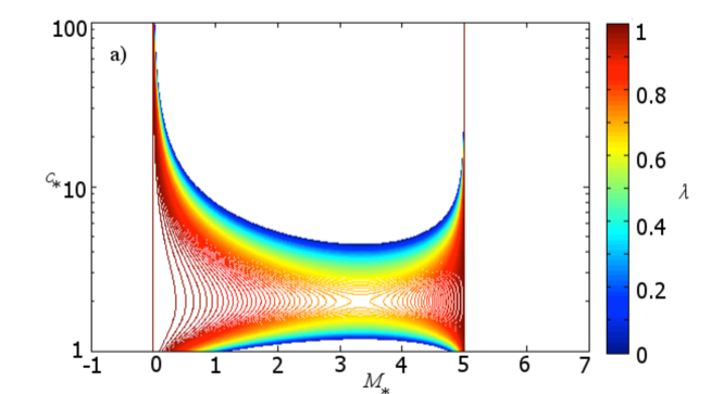
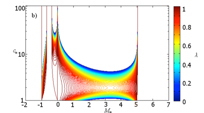
Figure 1: The regions in the $M_{*}$-$c_{*}$ space where the sonic locus can exist: a) in the presence of only friction losses, $c_{f}=0.01$, $c_{h}=0$, and b) when both heat and friction losses are present, $c_{f}=0.01$, $c_{h}=1.5c_{f}$. The lines in the figures are the iso-lines of $\lambda$ taken with step $0.01$.

In terms of our new variables, the sonic locus is fixed and determined exactly by $z=z^{\prime}=0$ at any parameters. Moreover, the singularity is no longer present in the system. More precisely, the singularity is reflected by the requirement that the branch of the square root of $z$ must change as one crosses the sonic locus. This procedure is numerically benign. Thus, we solve (58-60) with the corresponding boundary and sonic conditions, provided the sonic point exists. The non-singular character of the system allows one to calculate the solution with high precision. The goal is to find such a $D$ that the solution of equations (58-60) satisfies the boundary conditions at the shock and at $\xi=-\infty$ and to study the dependence of the detonation speed on the loss factors $c_{f}$ and $c_{h}$ assuming that other parameters are fixed. If there is a sonic point, we require that the sonic conditions $z=z^{\prime}=0$ are satisfied within machine precision. If there is no sonic point, the condition at the left boundary of the domain is imposed that both $u$ and $1-\lambda$ are close to zero within $10^{-10}$. Any changes in $c_{f}$ within the machine precision result in the changes of $u$ and $1-\lambda$ at infinity within $10^{-10}$, so that requiring even smaller errors is not feasible.

The new numerical algorithm works as follows. We first fix $E,$ $Q,$ $\gamma$ and the ratio $c_{f}/c_{h}$. The latter is essentially a constant for a given mixture, as seen from (25). Then, for every given $D\in[c_{a},D_{\mathrm{CJ}}]$, we look for the $c_{f}$ that provides a smooth solution to our boundary value problem. Here $c_{a}$, the sound speed in the ambient state, is equal to $\sqrt{\gamma}$ in our scales. The calculations show that there are two possible cases. If the detonation speed is less than $D_{\mathrm{CJ}}$, but greater than some value $D_{s}$, which is constant for the given set of parameters, then there is a sonic point inside the reaction zone. On the other hand, if $D\in(c_{a},D_{s})$, then there exist smooth solutions that satisfy the boundary conditions and remain subsonic from the shock down to $\xi=-\infty$.

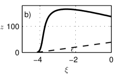
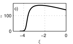
Figure 2: Profiles of $z$ in the shooting method for $D=0.8D_{\mathrm{CJ}}$ and various $c_{f}$: a) - $c_{f}=0.01$; b) - $c_{f}=0.006$; c) - $c_{f}=0.007$. Here $E=30,\;Q=20,\;\gamma=1.2$ and $c_{h}=0$.

The possible outcomes of the numerical search for $c_{f}$ for a given $D$ are shown in Fig. 2. The figures are computed by shooting from the shock to the sonic point with various $c_{f}.$ The Matlab ode15s solver with a reference tolerance value of $10^{-13}$ is used. In Fig. 2a), one can see the profile of $z$ for $c_{f}$ that is too large. Here, $z$ reaches its minimum value, but this value is positive. At $\xi$ less than the minimum point, $z$ together with $u$ and $p$ begin to grow without bound. For the exact solution, we expect $z$ to vanish at the minimum point. Hence, to measure the closeness of the computed profile to the exact solution, we define the error function, $\epsilon$, to be the minimum value of $z$. On the other hand, if $c_{f}$ is too small, then $z$ will reach zero with a positive slope, as in Fig. 2b). This means that condition (68) is not satisfied and $u$ will blow up because of the infinite derivative at the sonic point. In this case, we define $\epsilon$ to equal the derivative of $z$ at the sonic point. Then we find the minimum value of $\epsilon(c_{f})$ using Matlab’s FminSearch operator with a tolerance value of $10^{-13}$. The minimum value of $\epsilon=0$ corresponds to Fig. 2c). This case is the one that satisfies condition (68) and the corresponding $c_{f}$ is the proper value for the given detonation speed. At this value of $c_{f}$, we switch to the second branch of $\sqrt{z}$ and continue the calculations on the other side of the sonic point until $\xi=-\infty$.

For $D<D_{s}$, such numerical algorithm shows that there exists no $c_{f}$ that gives $\epsilon(c_{f})=0.$ However, smooth and bounded subsonic solutions still exist, i.e. $z$ remains positive in $(-\infty,0)$ and $u(-\infty)=0$. Such solutions are investigated below. The shooting from the shock gives three possibilities, as shown in Fig. 3a). If $c_{f}$ is too large, then $z$ passes its minimum point and then grows to infinity (solid line). If $c_{f}$ is too small, then again $z$ reaches the zero value with a non-zero slope, which means the blow-up of velocity (dash-dot line). However, instead of the behaviour in Fig. 2c), here we obtain the dashed line in the middle, which is the solution with a bounded value of $z$ at $\xi=-\infty$. This solution is possible only in the case when $u(-\infty)=0$, since it is the only equilibrium state for equations (58-60). It is important to note that the kinks in the curves in Fig. 3b) indicate a smooth, but rapid change in the solution. It occurs due to the exponentially sensitive terms in the governing equations.

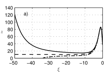
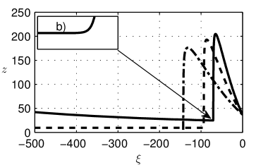
Figure 3: Profiles of $z$ in the shooting process at $D=0.4D_{\mathrm{CJ}}$, $c_{h}=0$, $Q=20$, $\gamma=1.2$ and various $c_{f}$: $c_{f}=0.01$ (solid), $c_{f}=0.0022$ (dash), $c_{f}=0.0011$ (dash-dot); a) $E=5$ and b) $E=30$.

4.2 Solutions in the presence of both heat and friction losses

If $D_{s}<D<D_{\mathrm{CJ}}$, the steady-state solution passes through a sonic point, where conditions (68) must be satisfied. Imposition of these conditions yields the exact value of the detonation speed for the given loss terms. The presence of a sonic point is a special feature that constrains the solutions to a particular form, essentially independent of the boundary conditions at infinity. However, if $c_{a}<D<D_{s}$, the sonic point and hence the constraint disappears and the nature of the solutions changes, since now the downstream boundary condition determines the detonation speed [2, 3]. The solutions connect the Rankine-Hugoniot conditions at the shock, $\xi=0$, and some appropriate conditions at $\xi=-\infty$. In the reference frame of the shock, the flow remains subsonic throughout. As a consequence of the loss of the sonic constraints, which if present pin down the solution to yield a unique $c_{f}$ for a given $D$, a degree of freedom is gained. The only condition at $\xi=-\infty$ that can justifiably be imposed is $u=0$, which leaves one condition there to be free. This can either be pressure or temperature; the density at infinity is the same as in the ambient gas, which follows easily from the continuity equation (37). As a result of this degree of freedom, the case $c_{a}<D<D_{s}$ yields a set-valued solution in which the pressure at $\xi=-\infty$ is allowed to vary in some range. That is, given the shock conditions and $u\left(-\infty\right)=0$, for any chosen $D\in\left(c_{a},D_{s}\right)$, there exists a continuous range of $c_{f}$ (at fixed $c_{f}/c_{h}$) that yields a smooth and bounded solution of (58-60). The transition from the single-valued to set-valued solutions is shown in Fig. 4a). For the existence of the set-valued solutions, the pressure at infinity cannot simply be arbitrary. For a fixed $D<D_{s}$, as we vary $c_{f}$, the flow variables $p$ and $T$ at $\xi=-\infty$ vary as well (but $u=0$ and $\lambda=1$ remain the same). The range of the corresponding variation of $p\left(-\infty\right)$ is shown in Fig. 4b). It is important to keep in mind that in Fig. 4b), $c_{f}$ is not fixed, but rather varies in the range seen in Fig. 4a) for any given $D$. An interesting feature of the pressure at infinity is that its maximum value appears to coincide with the moment when the sonic locus is exactly at infinity. This is the case in all of the calculations that we have performed. As the velocity decreases further, the pressure at infinity (hence the temperature there as well) begins to drop. Therefore, the numerical calculations indicate that the onset of the set-valued solutions coincides with the maximum temperature (or pressure) in the products.

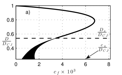
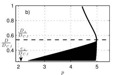
Figure 4: a) The dependence of the detonation speed, $D$, on the loss factor, $c_{f}$; b) the pressure at infinity, $p\left(-\infty\right)$, for the $D$-$c_{f}$ dependence shown in a). In both cases $E=30$.

In Fig. 4 and all of the calculations below, unless otherwise indicated, the following parameters are fixed: $Q=20,\;\gamma=1.2$ and $c_{h}=0.4c_{f}$.

For completeness, we analyze the structure of the solutions on the function-valued branch where they correspond to the self-sustained detonations. One of the main problems in the analysis is to understand the relative role of the three driving physical processes: chemical reaction, friction and heat transfer. While the roles of the chemical reaction and heat transfer are relatively simple, the former always contributing energy and the latter always taking it away, the role of friction is more complex. The friction term, $f$, changes its sign with velocity, which can result in momentum gain as opposed to momentum loss when $u<0$. More importantly, however, the friction results in heating of the gas and thus acts as a heat source. This is seen in the energy equation (8). Here, we analyze the role of these terms in more detail by evaluating their contributions to the fluid acceleration, $\mathrm{d}u/\mathrm{d}\xi$, and to the temperature gradient, $\mathrm{d}T/\mathrm{d}\xi$.

If one writes out the equation for $u\left(\xi\right)$ from (42) as follows

$$\frac{\mathrm{d}u}{\mathrm{d}\xi}=\frac{1}{\left(u-D\right)^{2}-c^{2}}\left[-\left(\gamma-1\right)Q\omega-\frac{\left(\gamma u-D\right)}{\rho\phi}f+\frac{\left(\gamma-1\right)}{\rho\phi}h\right],$$ (69)

then it is clear that the behaviour of $u$ depends on the competition between the heat release, friction and heat loss. Recall that $f=c_{f}\rho u\left|u\right|$, $h=c_{h}\left|u\right|\left(T-1\right)$ and that $c_{h}=\beta c_{f}$ for some fixed $\beta$ ($\beta=0.4$ in most of our calculations).

It is interesting that $\gamma u-D$ in the friction term in (69) can take either sign. To evaluate it at the shock, we use the jump condition (20),

$$\gamma u_{s}-D=c_{a}\left(\gamma\frac{u_{s}}{c_{a}}-M_{a}\right)=c_{a}\left[\frac{\left(\gamma-1\right)M_{a}^{2}-2\gamma}{\left(\gamma+1\right)M_{a}}\right].$$ (70)

Therefore, $\gamma u_{s}-D<0$ if $M_{a}^{2}<2\gamma/\left(\gamma-1\right)$ and $\gamma u_{s}-D>0$ otherwise. In the tail of the reaction zone, where $u$ is small, $\gamma u-D<0$. Thus, for sufficiently strong detonations, the factor $\gamma u-D$ will change signs somewhere in the reaction zone. For sufficiently large $M_{a}$, we obtain that near the shock $\left(\gamma u-D\right)f>0$ and, therefore, since $\left(u-D\right)^{2}-c^{2}<0$ near the shock, the friction term leads to a velocity decrease as does the heat release term. The effect of the heat loss term is the opposite. At small enough detonation Mach numbers, however, the role of the friction term is reversed because the sign of $\gamma u-D$ changes near the shock. The reversal of the sign of $\gamma u-D$ seems always to occur well above the turning point of the $D-c_{f}$ curve and hence no significant qualitative change to the solution results. However, we have not explored the whole range of possibilities and the consequences of this sign change. In the cases we considered, there seems to be no significant effect.

In the set-valued part of the solution, the flow is fully subsonic. Therefore, $\left(u-D\right)^{2}-c^{2}<0$ everywhere. If the numerator on the right-hand side of (69) is also negative, then $u^{\prime}>0$, such that $u$ decreases as $\xi$ tends to $-\infty$. Suppose now that $u$ reaches its zero value. At that point, both $f$ and $h$ vanish, but $\omega$ is still non-zero. Therefore, $u$ will continue to decrease. Once $u$ becomes negative, the $h$ term retains its sign, i.e., it remains positive, but the $f$ term now switches sign. Instead of acting with the reaction term, which it did for $u>0$, now the friction term acts with the heat loss term. As the magnitude of the negative velocity keeps increasing, the friction and heat loss terms in the numerator of (69) will balance the diminishing reaction rate term at some point. Downstream of that point, it is the loss terms that dominate, while the reaction term stops playing any significant role. Since the sign of $u^{\prime}$ is now reversed, $u$ begins to increase toward zero. The trend is asymptotic, since at small $u$, the right-hand side of (69) is essentially proportional to $-\left|u\right|$, such that $u=0$ near infinity is a (half-) stable fixed point.

The equation for temperature is more revealing. Using $T^{\prime}=p^{\prime}v+pv^{\prime}$, $v=\left(D-u\right)/D$ and (42-43) to calculate $p^{\prime}$ and $u^{\prime}$, we find that

$$\frac{\mathrm{d}T}{\mathrm{d}\xi}=-\frac{\left(\gamma-1\right)Dv}{\gamma\left(1-M^{2}\right)M^{2}c^{2}}\left[\left(1-\gamma M^{2}\right)\left(Q\omega-\frac{h}{\rho\phi}\right)+\left(1-\frac{\gamma u}{D}M^{2}\right)\frac{Df}{\rho\phi}\right].$$ (71)

Here, $M=\left(D-u\right)/c$ is the local Mach number of the flow. Because the factor in front of the brackets in (71) is always negative, the rise of the temperature in the reaction zone is due to the positive terms in the brackets. Depending on whether $M^{2}$ is smaller or larger than $1/\gamma$, the heat release term is seen to contribute to the temperature increase or decrease, respectively. The latter happens when the cooling by expansion dominates over heating, a situation well known in ideal detonation theory. This dual role of heat release leads to a temperature maximum in the reaction zone. The heat loss term is seen to have an effect opposite to that of the heat release. Note that the roles of chemical heat release and the heat transfer are always opposite and they switch signs where $1-\gamma M^{2}$ switches signs.

When $u>0$, the friction term leads to the local heating of the gas if $1-\gamma uM^{2}/D>0$ and to cooling it otherwise. Because $f=c_{f}\rho u\left|u\right|$, when $u\leq 0$, we obtain that $1-\gamma uM^{2}/D>0$, but $f<0$. Therefore, in the latter case, the friction cools the gas. Note that this temperature decrease is local and is not that of a fluid particle. For the latter, its rate of temperature change is $u\mathrm{d}T/\mathrm{d}\xi$, the contribution to which by friction will remain positive when $u$ changes sign.

Immediately at the shock, the jump conditions yield

$$\frac{\gamma u_{s}}{D}=\frac{\gamma u_{s}/c_{a}}{D/c_{a}}=\frac{2\gamma}{\gamma+1}\frac{M_{a}^{2}-1}{M_{a}^{2}}$$

and

$$M_{s}^{2}=\frac{2+\left(\gamma-1\right)M_{a}^{2}}{2\gamma M_{a}^{2}-\left(\gamma-1\right)}.$$

A little bit of algebra shows that

$$1-\frac{\gamma u_{s}}{D}M_{s}^{2}=\frac{4\gamma}{\left(\gamma+1\right)M_{a}^{2}\left(2\gamma M_{a}^{2}-\left(\gamma-1\right)\right)}\left[M_{a}^{4}-\frac{3\left(2-\gamma\right)}{4}M_{a}^{2}+1\right].$$ (72)

Thus, the sign of the left-hand side is controlled by the expression in the brackets, which is positive for reasonable $\gamma$. Then, in the region immediately after the shock, where $u>0$, the friction term always heats the gas. Again, the important question here is to determine which of the two heating processes, chemical or frictional, dominates. In order to answer this question, we plot the terms in (71) that represent various physics, at two different values of the detonation speed, one close to $D_{\mathrm{CJ}}$ and one substantially below $D_{\mathrm{CJ}}$ as shown in Fig. 5. As expected, when $D/D_{\mathrm{CJ}}=0.95$ the losses are small and the dominant role is played by the reaction heating the gas and thus driving the detonation wave. In contrast, at large velocity deficits, such as $D/D_{\mathrm{CJ}}=0.6$, frictional heating is seen to dominate in the large region immediately behind the shock. Comparison of the magnitudes of the friction terms in (71) for these two cases shows that they are substantially similar (approximately $0.4$ and $0.1$, the difference following from an approximately two-fold decrease in velocity). The reaction rate term, in contrast, decreases by orders of magnitude in the vicinity of the shock, as a result of the exponential sensitivity of the rate function to temperature. Thus, at low detonation velocities, the dominant role of the frictional heating is a result of the reaction becoming negligible. However, as the friction heats the gas, the reaction “switches on” at some distance from the shock.

Thus, the propagation mechanism of low-velocity detonation involves the shock-driven flow acceleration that leads to the frictional heating of the gas that triggers the chemical energy release that, in turn, drives the shock. The frictional heating in this mechanism is acting as an intermediary facilitating the onset of chemical energy release behind the shock, which itself is not strong enough to trigger the reaction. We should note that the heat loss term in this early stage of the process is negligible.

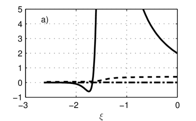
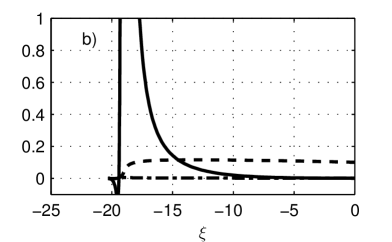
Figure 5: The profiles of various terms contributing to the temperature evolution in (71), $\mathcal{R}=\left(1-\gamma M^{2}\right)Q\omega$ (solid), $\mathcal{F}=D\left(1-\gamma uM^{2}/D\right)f/\left(\rho\phi\right)$ (dash) and $\mathcal{H}=\left(1-\gamma M^{2}\right)h/\left(\rho\phi\right)$ (dash-dot) at: a) $D/D_{\mathrm{CJ}}=0.95$ and b) $D/D_{\mathrm{CJ}}=0.6$.

In Fig. 6, we show the solution profiles at three different levels of the velocity deficit. As the deficit increases, the reaction is seen to start farther away from the shock, without substantially changing the width of the heat release zone (“fire”) with, however, a decreasing peak value of $\omega$. There is a clear build-up of pressure and temperature between the shock and the fire, which is due to frictional heating. The velocity profile tends to a square-wave like structure with a nearly constant value behind the shock that drops quickly in the fire zone to close to zero. We should note that $u=0$ only at $\xi\to-\infty$ over a long relaxation tail that extends from about $\xi\approx-20$. The relaxation region is many orders of magnitude longer than the region where most of the energy is released. We show an example in Fig. 7, where the $\xi$ scale is logarithmic. It can be seen that the relaxation of velocity from the negative values back to zero takes place over a 100 times longer distance than the distance from the shock to the fire. Although most of the figures below show only the region close to the shock, in all of the results presented here, the calculations are carried out to such long distances to verify that the velocity has indeed reached a value close to zero.

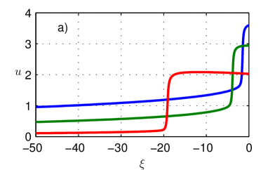
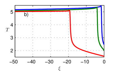
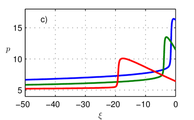
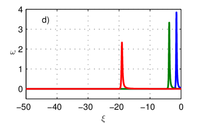
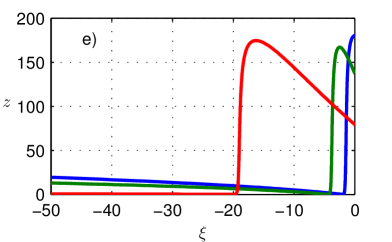
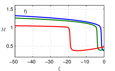
Figure 6: The profiles of: a) velocity, b) temperature, c) pressure, d) reaction rate, e) $z$ and f) Mach number relative to the shock at: $D/D_{\mathrm{CJ}}=0.95$ (blue), $0.8$ (green) and $0.6$ (red).

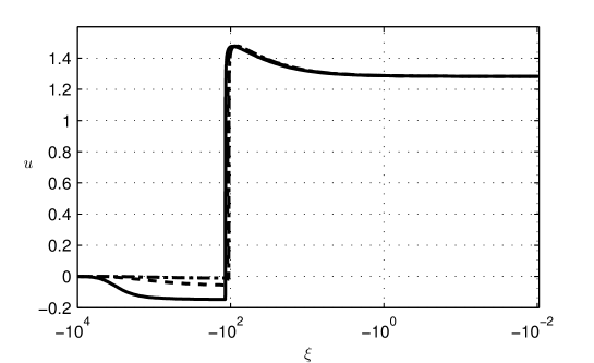
Figure 7: The velocity profiles at $D/D_{\mathrm{CJ}}=0.45$ and at three different values of $c_{f}$ in the set-valued region: two near the edges of the region, $c_{f}=0.0019$ (solid), $c_{f}=0.0022$ (dash-dot) and one in the middle, $c_{f}=0.0021$ (dash).

What is interesting and important in comparing the nature of the self-sustained and set-valued solutions is the fact that the self-sustained solutions do not require any boundary condition at infinity. In self-sustained solutions, the velocity relaxes to $u=0$ automatically, once the solution passes through the sonic point. It is therefore sufficient to require that the sonic point exists in the flow. In contrast, $u\left(-\infty\right)=0$ has to be imposed as a boundary condition in solutions without the sonic point. This observation highlights the special nature of self-sustained solutions. The presence of a sonic point is a rather strong constraint on a solution.

Next, we look at solutions without a sonic locus that exist at substantially larger velocity deficits. In Fig. 8, we show the solution profiles when the velocity is $D=0.45D_{\mathrm{CJ}}$, which is in the set-valued region. We take three values of $c_{f}$, two near the boundaries of the set-valued region and one in between, and plot the corresponding solution profiles. All of them look qualitatively similar. The right boundary is characterized by the absence of the negative phase of the velocity, which tends to zero asymptotically as $\xi\to-\infty$. The approach to the left boundary is more complicated and is shown in Fig. 9. In the set-valued region, at values of $c_{f}$, which are away from the boundaries, the local Mach number at infinity is $M_{b}=D/c\left(-\infty\right)<1$. As we approach the left boundary of the region, $M_{b}$ remains substantially below unity until we get very close to the left boundary of $c_{f}$, which is denoted as $c_{fl}$. There is a sharp boundary layer at $c_{fl}$ where $M_{b}$ starts to increase. We note that at $c_{f}<c_{fl}$, the steady-state solution does not exist and the solutions of the governing ODE system (for the original variables) blow up as a result of $1-M^{2}$ becoming zero. This may explain the trend seen just to the right of $c_{f}=c_{fl}$.

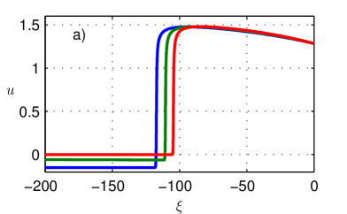
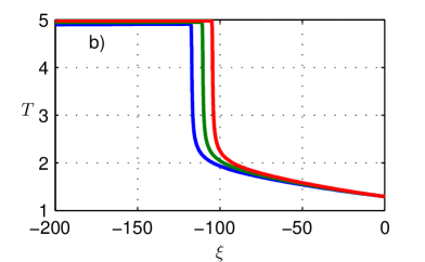
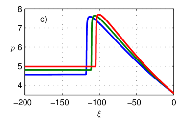
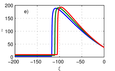
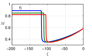
Figure 8: The solution profiles at a fixed $D/D_{\mathrm{CJ}}=0.45$ in the set-valued region: a) velocity, b) temperature, c) pressure, d) reaction rate, e) $z$ and f) Mach number at three different values of $c_{f}$: $c_{f}=0.0019$ (blue), $c_{f}=0.0021$ (green) and $c_{f}=0.0022$ (red).

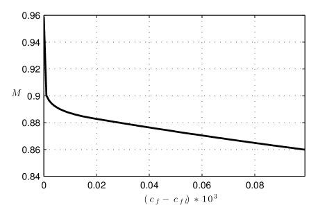
Figure 9: The profile of $M_{b}=D/c\left(-\infty\right)$ as a function of $c_{f}$ at $D/D_{\mathrm{CJ}}=0.45$ as $c_{f}$ approaches the left boundary of the set-valued region, $c_{fl}$. Within about $10^{-8}$ of the boundary, the far-field Mach number remains below $1$ although it does show a tendency towards $1$.

In the next set of calculations, we look at the structure of the steady-state solutions when $c_{f}$ is fixed and $D$ is allowed to take values in the set-valued region as well as on the top branch of the $D$-$c_{f}$ dependence. In Fig. 10, we show such profiles, which coexist for the same set of parameters describing an explosive mixture and a porous medium. Comparing Figs. 6, 8 and 10, we notice that the drop in detonation velocity at a given $c_{f}$ has a much more pronounced effect on the extent and the structure of the solution profiles than the variations of $c_{f}$ at a given velocity.

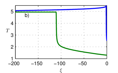
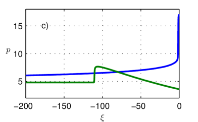
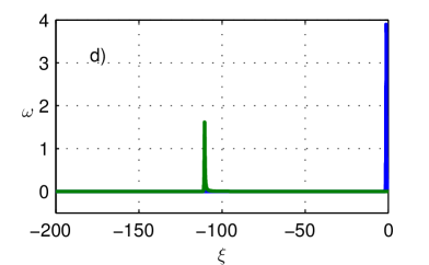
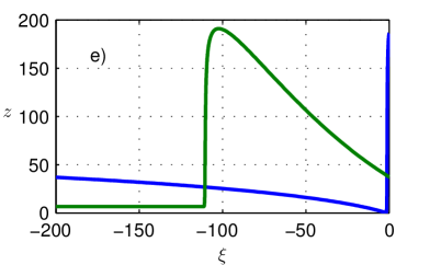
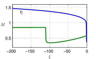
Figure 10: The solution profiles at a fixed $c_{f}=0.0021$ and: at $D/D_{\mathrm{CJ}}=0.97$ (blue) and at $D/D_{\mathrm{CJ}}=0.45$ (green).

The effect of the activation energy on the solutions is shown in Fig. 11a). The behaviour of the top part of the dependence is as expected: as the activation energy increases, the turning point tends to smaller values of $c_{f}$ and larger values of $D$. With increasing $E$, the set-valued region becomes significantly narrower, such that at a given $D$, the range of $c_{f}$ for which the steady-state solution exists, is diminished. However, note that for a given $c_{f}$ in the set-valued range, the variations of $D$ are still significant, as the region becomes nearly vertical. The latter is important in the sense that if one chooses the porous medium to yield this particular value of $c_{f}$, then the range of possible steady-state detonation velocities is still large.

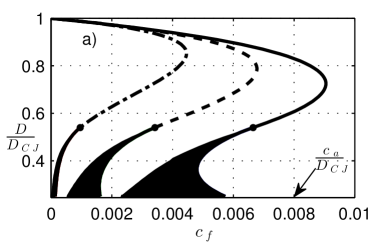
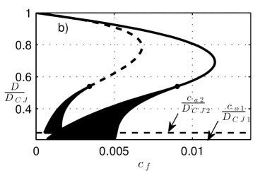
Figure 11: The effect of activation energy and the ratio of specific heats: a) $\gamma=1.2$, $E=25$ (solid), $E=30$ (dash), and $E=40$ (dash-dot); b) $E=30$, $\gamma=1.2$ (solid) and $\gamma=1.3$ (dash).

The adiabatic index turns out to have a strong influence on the $D$-$c_{f}$ dependence as well as shown in Fig. 11b). Changing $\gamma$ from $1.2$ to $1.3$ shifts the dependence toward smaller $c_{f}$ and the turning point toward larger $D$. In addition, the set-valued part becomes narrower with increasing $\gamma$. The bottom limit of the dependence changes as well due to the change in the ambient sound speed.

The ratio $\beta=c_{h}/c_{f}$ is fixed at $0.4$ in most calculations above. The self-sustained part of the solution is less affected by the change of $\beta$ than is the set-valued part; this is shown in Fig. 12. Note that if the heat loss term is ignored, then no set valued solutions exist and we obtain the familiar Z-shaped curve.

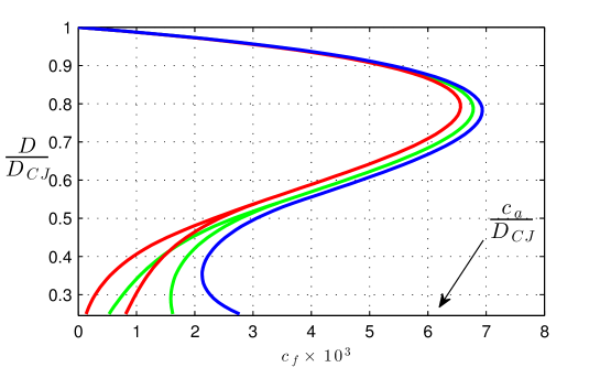
Figure 12: The effect of $\beta=c_{h}/c_{f}$: $\beta=0$ (blue), $\beta=0.4$ (green), $\beta=1$ (red). The set-valued areas are not filled to avoid overlaps, but it should be understood that the region between the red (correspondingly, green) curves is set-valued. When $\beta=0$, the solution is a curve. In all cases $E=30,\;Q=20,\;\gamma=1.2$.

5 Conclusions

In this work, we revisited the classical problem of one-dimensional gaseous detonation in the presence of losses of heat and momentum. In particular, we analyzed the existence and structure of the steady-state solutions of the one-dimensional reactive Euler equations for gaseous detonation propagating in the interstitial space between packed spherical particles. The friction force was assumed to be proportional to the square of the flow velocity and the heat loss to the temperature difference between the gas and the particles. The heat transfer was assumed to be purely convective, such that it vanished in the absence of flow.

Our main finding is that the steady-state solutions have a set-valued character at sufficiently low speeds of detonation when the flow downstream of the shock is entirely subsonic relative to the shock. The vanishing velocity at the downstream infinity with no additional constraints on the solution results in the existence of a continuous spectrum of detonation velocities all corresponding to the steady-state solution of the governing equations. For any given loss factors, such solutions are found to exist provided that both the friction and heat losses are considered and provided that the detonation velocity is sufficiently low, i.e., the velocity deficit is large. This result, that the nonlinear eigenvalue problem has in general both a discrete and a continuous spectrum, is in contrast to previous findings for the problem, which predicted only a finite number of discrete values of the detonation speed at any given loss coefficient.

Regarding the solutions with regions of negative velocity in the reaction zone, we find that such regions cannot exist in self-sustained waves (i.e. in the presence of the sonic point). They also do not exist if one neglects heat losses, at least when only convective heat loss is considered. Only in the presence of heat losses and only if the solution contains no sonic point does the flow velocity take negative values somewhere in the reaction zone. The latter situation corresponds to the existence of the set-valued region in the $D-c_{f}$ plane. The set-valued solutions arise because of the sonic constraint disappearing from the solution and an additional degree of freedom appearing as a result. This degree of freedom is the pressure or temperature at infinity, which if imposed leads to the usual multiple but finite number of solutions. This creates an interesting possibility that the detonation speed can be controlled by the downstream pressure, a situation akin to the overdriven case wherein a piston pushing the products downstream controls the detonation velocity. However, the difference in the present case is that the velocity is less than the CJ velocity.

Another new result of this work is a formulation of governing equations in terms of new dependent variables that yield an ODE system for steady-state solutions without sonic singularity. The new formulation allows us to eliminate completely the numerical difficulties associated with the integration across the sonic singularity. Our approach can be generalized and we believe will be useful in other, even more complex problems of determining the detonation eigenvalue solutions.

The existence of multiple steady-state solutions for the non-ideal detonation raises an important question about their stability. Numerical evidence points to a destabilizing role of losses, which is similar to the role of curvature in expanding spherical/cylindrical detonations. However, detailed theoretical study of stability of these solutions is still required.

References

- [1] J. B. Bdzil and D. S. Stewart. Theory of detonation shock dynamics. In Shock Waves Science and Technology Library, Vol. 6, pages 373–453. Springer, 2012.
- [2] I. Brailovsky and G. Sivashinsky. Hydraulic resistance and multiplicity of detonation regimes. Combustion and flame, 122(1):130–138, 2000.
- [3] I. Brailovsky and G. Sivashinsky. Effects of momentum and heat losses on the multiplicity of detonation regimes. Combustion and flame, 128(1):191–196, 2002.
- [4] J. P. Dionne, H. D. Ng, and J. H. S. Lee. Transient development of friction-induced low-velocity detonations. Proceedings of the Combustion Institute, 28(1):645–651, 2000.
- [5] W. Döring. Uber den detonationvorgang in gasen. Annalen der Physik, 43(6/7):421–428, 1943.
- [6] B.S. Ermolaev, B.A. Khasainov, and K.A. Sleptsov. Numerical simulation of modes of combustion and detonation of hydrogen-air mixtures in porous medium in the framework of the mechanics of two-phase reaction mediums. Russian Journal of Physical Chemistry B, 5:1007–1018, 2011.
- [7] H. Eyring, R. E. Powell, G. H. Duffy, and R. B. Parlin. The stability of detonation. Chemical Reviews, 45:69–181, 1949.
- [8] L. M. Faria and A. R. Kasimov. On computing self-sustained shock-wave solutions of hyperbolic balance laws. In preparation, 2013.
- [9] W. Fickett and W. C. Davis. Detonation: theory and experiment. Dover Publications, 2011.
- [10] M.A. Goldshtik. Transfer processes in granular layer. Institute of Thermophysics of the Siberian Branch of the USSR Academy of Science, Novosibirsk, 1984.
- [11] A. J. Higgins. Steady one-dimensional detonations. In Shock Waves Science and Technology Library, Vol. 6, pages 33–105. Springer, 2012.
- [12] J. H. S. Lee, R. Knystautas, and C. K. Chan. Turbulent flame propagation in obstacle-filled tubes. In Symposium (International) on Combustion, volume 20, pages 1663–1672. Elsevier, 1985.
- [13] G. A. Lyamin, V. V. Mitrofanov, A. V. Pinaev, and V. A. Subbotin. Propagation of gas explosion in channels with uneven walls and in porous media. Dynamic Structure of Detonation in Gaseous and Dispersed Media, Kluwer Academ., Netherlands, pages 51–75, 1991.
- [14] G. A. Lyamin and A. V. Pinaev. Combustion regimes for gases in an inert porous material. Combustion, Explosion, and Shock Waves, 22(5):553–558, 1986.
- [15] A. V. Pinaev and G. A. Lyamin. Fundamental laws governing subsonic and detonating gas combustion in inert porous media. Combustion, Explosion, and Shock Waves, 25(4):448–458, 1989.
- [16] J. von Neumann. Theory of detonation waves. Office of Scientific Research and Development, Report 549. Technical report, National Defense Research Committee Div. B, 1942.
- [17] W. W. Wood and J. G. Kirkwood. Diameter effect in condensed explosives. the relation between velocity and radius of curvature in the detonation wave. J. Chem. Phys., 22:1920–1924, 1954.
- [18] Y. B. Zel’dovich. On the theory of propagation of detonation in gaseous systems. J. Exp. Theor. Phys., 10(5):542–569, 1940.
- [19] Y. B. Zel’dovich, A. A. Borisov, B. E. Gel’fand, S. M. Frolov, and A. E. Mailkov. Nonideal detonation waves in rough tubes. Dynamics of Explosions, AIAA Progress in Astronautics and Aeronautics, AIAA, NY, 114:211–231, 1988.
- [20] Y. B. Zel’dovich, B. E. Gel’fand, Y. M. Kazhdan, and S. M. Frolov. Detonation propagation in a rough tube taking account of deceleration and heat transfer. Combustion, Explosion, and Shock Waves, 23(3):342–349, 1987.
- [21] Y. B. Zel’dovich and A. S. Kompaneets. Theory of Detonation. New York: Academic Press, 1960.