Special Algorithm for Stability Analysis
of Multistable Biological Regulatory Systems

Abstract

We consider the problem of counting (stable) equilibriums of an important family of algebraic differential equations modeling multistable biological regulatory systems. The problem can be solved, in principle, using real quantifier elimination algorithms, in particular real root classification algorithms. However, it is well known that they can handle only very small cases due to the enormous computing time requirements. In this paper, we present a special algorithm which is much more efficient than the general methods. Its efficiency comes from the exploitation of certain interesting structures of the family of differential equations.

Key words: quantifier elimination, root classification, biological regulation system, stability

1 Introduction

Modeling biological networks mathematically as dynamical systems and analyzing the local and global behaviors of such systems is an important method of computational biology. The most concerned behaviors of such biological systems are equilibrium, stability, bifurcations, chaos and so on.

Consider the stability analysis of biological networks modeled by autonomous systems of differential equations of the form $\dot{{\mathbf{x}}}={\mathbf{f}}\left({\mathbf{u}},{\mathbf{x}}\right)$ where ${\mathbf{x}}=\left(x_{1},\ldots,x_{n}\right)$,

$${\mathbf{f}}\left({\mathbf{u}},{\mathbf{x}}\right)=\left(f_{1}\left({\mathbf{u}},x_{1},\ldots,x_{n}\right),\ldots,f_{n}\left({\mathbf{u}},x_{1},\ldots,x_{n}\right)\right)$$

and each $f_{k}\left({\mathbf{u}},x_{1},\ldots,x_{n}\right)$ is a rational function in $x_{1},\ldots,x_{n}$ with real coefficients and real parameter(s) ${\mathbf{u}}$. We would like to compute a partition of the parametric space of ${\mathbf{u}}$ such that, inside every open cell of the partition, the number of (stable) equilibriums of the system is uniform. Furthermore, for each open cell, we would like to determine the number of (stable) equilibriums.

Such a problem can be easily formulated as a real quantifier elimination problem. It is well known that the real quantifier elimination problem can be carried out algorithmically. [61, 18, 3, 46, 47, 48, 31, 33, 34, 20, 50, 51, 52, 7, 8, 9, 11, 12, 26, 16, 57, 58, 14, 42, 10, 15]. There are several software systems such as QEPCAD [20, 35, 11, 13], Redlog [28], Reduce (in Mathematica) [55, 56] and SyNRAC [1]. Hence, in principle, the stability analysis of regulation system the above system can be carried out automatically using those software systems. However, it is also well known that the complexity [25, 7] of those algorithms are way beyond current computing capabilities since those algorithms are for general quantifier elimination problems.

The stability analysis is a special type of quantifier elimination problem, in particular, real root classification. Hence, it would be advisable to use real root classification algorithms [69, 70]. In fact, [62, 63], [65] and [66] tackled the stability analysis problem using DISCOVERER [67]. They were able to tackle a specialized simultaneous decision problem ($n=6$ and $c=2$) [22] in $55,000$ secs [66]. However, the real root classification software could not go beyond these, due to enormous computing time/memory requirements.

In this paper, we consider the problem of counting (stable) equilibriums of an important family of algebraic differential equations modeling multistable biological regulation systems, called MSRS (see Definition 1). In fact, the family is a straightforward generalization of several interesting classes of systems in the literature [22, 23, 24]. The family of differential equations has the form $\dot{{\mathbf{x}}}={\mathbf{f}}\left(\sigma,{\mathbf{x}}\right)$ where ${\mathbf{f}}$ is a real function determined by certain real functions $l\left(z\right)$, $g\left(z\right)$, $h\left(z\right)$ and $P\left({\mathbf{x}}\right)$ and parameterized by a real parameter $\sigma$.

We present a special algorithm which is much more efficient than the general root classification algorithm. The efficiency of the special algorithm comes from the exploitation of certain interesting structures of the differential equation under investigation such as

1. the eigenvalues of the Jacobian at every equilibrium are all real, see Theorem 1;

2. every equilibrium of the system is made up of at most two components, see Theorem 2;

3. the eigenvalues of the Jacobian at every equilibrium have certain structures (see Theorems 3 and 4), aiding the determination of stability of an equilibrium (see Corollary 1).

The special algorithm can handle much larger system than the general root classification algorithm. For example, it can handle a specialized simultaneous decision problem ($n=11$ and $c=8$) in several seconds.

We remark that our work can be viewed as following the numerous efforts in applying quantifier elimination to tackle problems from various other disciplines [44, 45, 30, 29, 43, 64, 39, 40, 71, 2, 62, 63, 17, 32, 65, 68, 54, 59, 66, 53].

The paper is organized as follows. Section 2 provides a precise statement of the problem. Section 3 reviews a general algorithm based on real root classification. Section 4 proves several interesting structures of the problem. Section 5 gives a special algorithm that exploits the structure proved in Section 4. Section 6 presents the experimental timings and compares them to those of a general algorithm.

2 Problem

In this section, we give a precise and self-contained description of the problem. First we introduce a family of differential equations that we will be considering.

Definition 1 ( MultiStable Regulatory System).

A system of ordinary differential equations

$$\frac{dx_{1}}{dt} =f_{1}\left(\sigma,x_{1},\ldots,x_{n}\right)$$

$$\vdots$$

$$\frac{dx_{n}}{dt} =f_{n}\left(\sigma,x_{1},\ldots,x_{n}\right)$$

is called a multistable regulatory system (MSRS) if $f_{k}$ has the following form

$$f_{k}\left(\sigma,x_{1},\ldots,x_{n}\right)=-l\left(x_{k}\right)+\sigma\frac{g\left(x_{k}\right)}{P\left(x_{1},\ldots,x_{n}\right)+h\left(x_{k}\right)}$$

where

1. $\sigma$ is a positive parameter;

2. The function $P$ is symmetric, that is,

   $$P\left(x_{1},\ldots x_{i},\ldots,x_{j},\ldots,x_{n}\right)=P\left(x_{1},\ldots x_{j},\ldots,x_{i},\ldots,x_{n}\right)$$

   for every $i,j$;

3. $\forall k\;\forall(x_{1},\ldots,x_{n})\in{\mathbb{R}}^{n}_{>0}\;\;\;P\left(x_{1},\ldots,x_{n}\right)+h\left(x_{k}\right)>0$;

4. $l\left(z\right)\neq 0$ and for every $\sigma\in{\mathbb{R}}_{>0}$, the function

   $$\sigma\frac{g\left(z\right)}{l\left(z\right)}-h\left(z\right)$$

   has at most one extreme point on the intended domain of $z$.

Example 1.

We present several examples of MSRS from cellular differentiation [22, 23, 24]. In fact, the above definition of MSRS is a straightforward generalization of those differential equations.

1. Simultaneous decision [22].

   $$\frac{dx_{k}}{dt}=-x_{k}+\sigma\frac{1}{1+\Sigma_{m=1}^{n}x_{m}^{c}-x_{k}^{c}}$$

   where the quantities $x_{1},...,x_{n}$ $(\in{\mathbb{R}}_{>0})$ denote the concentrations of $n$ proteins, $c$ ($\in{\mathbb{R}}_{>0}$) the cooperativity, and $\sigma$ ($\in{\mathbb{R}}_{>0}$) the strength of unrepressed protein expression, relative to the exponential decay. It is easy to verify that it is a MSRS with

   $$l\left(z\right)=z,\;g\left(z\right)=1,\;h\left(z\right)=-z^{c},$$

   $$P\left(x_{1},\ldots,x_{n}\right)=1+\Sigma_{m=1}^{n}x_{m}^{c}.$$

   The first graph in Figure 1 shows the graph of $\sigma\frac{g\left(z\right)}{l\left(z\right)}-h\left(z\right)$ for $c=4$ and $\sigma=1$.

2. Mutual inhibition with autocatalysis [23].

   $$\frac{dx_{k}}{dt}=-x_{k}+\alpha+\sigma\frac{x_{k}^{c}}{1+\Sigma_{m=1}^{n}x_{m}^{c}}$$

   where the quantities $x_{1},...,x_{n}$ $(\in{\mathbb{R}}_{>0})$ denote the concentrations of $n$ proteins, $c$ ($\in{\mathbb{R}}_{>0}$) the cooperativity, $\sigma$ ($\in{\mathbb{R}}_{>0}$) the relative speed for transcription/translation, and $\alpha$ ($\in{\mathbb{R}}_{\geq 0}$) the leak expression. It is easy to verify that it is a MSRS with

   $$l\left(z\right)=z-\alpha,\;g\left(z\right)=z^{c},\;h\left(z\right)=0,$$

   $$P\left(x_{1},\ldots,x_{n}\right)=1+\Sigma_{m=1}^{n}x_{m}^{c}.$$

   The second graph in Figure 1 shows the graph of $\sigma\frac{g\left(z\right)}{l\left(z\right)}-h\left(z\right)$ for $\alpha=1$, $c=2$ and $\sigma=1$.

3. bHLH dimerisation [23, 24].

   $$\frac{dx_{k}}{dt}=-x_{k}+\sigma\frac{x_{k}^{2}}{\frac{K_{2}}{a_{t}^{2}}\left(1+\Sigma_{m=1}^{n}x_{m}\right)^{2}+x_{k}^{2}}$$

   where the quantities $x_{1},...,x_{n}$ $(\in{\mathbb{R}}_{>0})$ denote the concentrations of $n$ proteins, $\sigma$ ($\in{\mathbb{R}}_{>0}$) the relative speed for transcription/translation, $K_{2}$ $(\in{\mathbb{R}}_{>0})$ the binding constant, and $a_{t}$ $(\in{\mathbb{R}}_{>0})$ the total quantity of activator. It is easy to verify that it is a MSRS with

   $$l\left(z\right)=z,\;g\left(z\right)=z^{2},\;h\left(z\right)=z^{2},$$

   $$P\left(x_{1},\ldots,x_{n}\right)=\frac{K_{2}}{a_{t}^{2}}\left(1+\Sigma_{m=1}^{n}x_{m}\right)^{2}.$$

   The third graph in Figure 1 shows the graph of $\sigma\frac{g\left(z\right)}{l\left(z\right)}-h\left(z\right)$ for $\sigma=1$.

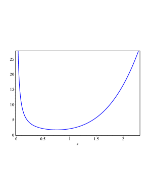
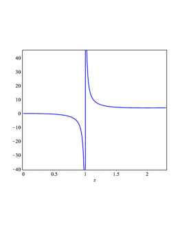
Figure 1: Graphs of $\sigma\frac{g\left(z\right)}{l\left(z\right)}-h\left(z\right)$ for the models in Example 1

Definition 2 (Equilibrium).

For given $\sigma$, an ${\mathbf{r}}\in{\mathbb{R}}_{>0}^{n}$ is called an equilibrium if

$$f_{1}\left({\mathbf{r}}\right)=\cdots=f_{n}\left({\mathbf{r}}\right)=0.$$

Notation 1 (Jacobian).

The Jacobian of ${\mathbf{f}}$ is denoted by

$$J_{\mathbf{f}}=\left[\begin{matrix}\frac{\partial f_{1}}{\partial x_{1}}&\cdots&\frac{\partial f_{1}}{\partial x_{n}}\\ \vdots&\ddots&\vdots\\ \frac{\partial f_{n}}{\partial x_{1}}&\cdots&\frac{\partial f_{n}}{\partial x_{n}}\end{matrix}\right].$$

Definition 3 (Stable).

An equilibrium ${\mathbf{r}}$ is called stable (more precisely, locally asymptotically stable) if all eigenvalues of $J_{\mathbf{f}}\left({\mathbf{r}}\right)$ have strictly negative real parts.

We are ready to state the problem that will be tackled in this paper. Informally, the problem is as follows. For given polynomials $l,g,h$ and $P$, we have a family of MSRS parameterized by $\sigma$. We would like to find a partition of $\sigma$ values into several intervals so that for all $\sigma$ in each interval the number of (stable) equilibriums is uniform. Furthermore, for each interval, we would like to determine the number of (stable) equilibriums. Now let us state the problem precisely.

Problem.

Devise an algorithm with the following specification.

1. Input: ${\mathbf{f}}=\left(f_{1},\ldots,f_{n}\right)\in\left({\mathbb{Q}}\left(\sigma,{\mathbf{x}}\right)\right)^{n}$ such that $\dot{\mathbf{x}}={\mathbf{f}}$ is a MSRS

2. Output:

   $B\in\mathbb{Z}[\sigma],$
   $I_{1},\ldots,I_{w-1}\in\mathbb{IQ}_{>0}$ (that is, closed intervals with positive rational endpoints) and
   $\left(e_{1},s_{1}\right),\ldots,\left(e_{w},s_{w}\right)\in\mathbb{Z}^{2}_{\geq 0}$
   such that

   1. $\forall j\in\{1,\ldots,w-1\},\;B$ has one and only one real root, say $\sigma_{j}$, in $I_{j}$,

   2. $\sigma_{1}<\cdots<\sigma_{w-1}$, and

   3. $\forall j\in\{1,\ldots,w\}\;\;\forall v\in\left(\sigma_{j-1},\sigma_{j}\right)\;\;E_{v}=e_{j}\;\wedge S_{v}=s_{j}$

   where

   1. $\sigma_{0}=0$, $\sigma_{w}=\infty$,

   2. $E_{v}$ ($S_{v}$) denotes the number of (stable) equilibriums of $\dot{\mathbf{x}}={\mathbf{f}}\left(v,{\mathbf{x}}\right)$

Example 2.

We illustrate the above input and output specification by an example, which is a specific simultaneous decision model ($n=4$ and $c=4$) as shown in Example 1.

1. Input: $f_{1},f_{2},f_{3},f_{4}$
   where $f_{k}=-x_{k}+\frac{\sigma}{1+x_{1}^{4}+x_{2}^{4}+x_{3}^{4}+x_{4}^{4}-x_{k}^{4}},\;\;k=1,\ldots,4$

2. Output:

   $B=\left(42755090541778564453125\sigma^{24}+\cdots-140737488355328\right)\left(\sigma-4\right)^{2}$,
   $I_{1}=[\frac{5}{4},\frac{21}{16}],\;\;I_{2}=[4,4],$
   $\left(e_{1},s_{1}\right)=\left(1,1\right),\;\;\left(e_{2},s_{2}\right)=\left(9,5\right),\;\;\left(e_{3},s_{3}\right)=\left(15,4\right)$

By Definition 1, the input system is

$$\frac{dx_{k}}{dt}=-x_{k}+\frac{\sigma}{1+x_{1}^{4}+x_{2}^{4}+x_{3}^{4}+x_{4}^{4}-x_{k}^{4}}.$$

The meaning of the output is as follows. Let $\sigma_{1}~{}(\approx 1.303331342)$ be the unique positive root of $B\left(\sigma\right)=0$ in $I_{1}$ and $\sigma_{2}~{}(=4)$ be the unique positive root of $B\left(\sigma\right)=0$ in $I_{2}$. Then the system has the following properties:

1. if $0<\sigma<\sigma_{1}$, then the system has exactly $1$ equilibrium and the equilibrium is stable;

2. if $\sigma_{1}<\sigma<\sigma_{2}$, then the system has exactly $9$ distinct equilibriums, $5$ of which are stable;

3. if $\sigma_{2}<\sigma<\infty$, then the system has exactly $15$ distinct equilibriums, $4$ of which are stable.

3 Review of General Algorithm

In this section, we briefly review a general algorithm [62, 63, 65, 66] for stability analysis based on real root classification. As stated in Section 1, the general algorithm works for systems with rational functions and thus can be applied to solve the Problem posted in last section for MSRS if all the involved functions, i.e., $l,g,h,P$, are polynomials.

Suppose we are given a system $\dot{{\mathbf{x}}}={\mathbf{f}}\left(\sigma,{\mathbf{x}}\right)$ where

$${\mathbf{f}}\left(\sigma,{\mathbf{x}}\right)=(f_{1}(\sigma,x_{1},\ldots,x_{n}),\ldots,f_{n}(\sigma,x_{1},\ldots,x_{n}))$$

and each $f_{k}(\sigma,x_{1},\ldots,x_{n})$ is a rational function. A sketch description of the general algorithm may be as follows.

1. Equate the numerators of all $f_{k}(\sigma,x_{1},\ldots,x_{n})$ to $0$, yielding a system of polynomial equations. To simplify the notations, we still use $\{f_{1}=0,\ldots,f_{n}=0\}$ to denote the equations. Note that there may be some constraints on the system. For example, the denominators of all $f_{k}$ should be nonzero, $\sigma$ and some variables should be positive, and so on. Therefore, we actually obtain a semi-algebraic system. Let us denote it by ${\mathcal{S}}$.

2. Compute the Hurwitz determinants $\Delta_{1},\ldots,\Delta_{n}$ of the Jacobian matrix $J_{\mathbf{f}}\left(\sigma,{\mathbf{x}}\right)$. Let $\det\left(\lambda I-J_{\mathbf{f}}\left(\sigma,{\mathbf{x}}\right)\right)=b_{n}\lambda^{n}+b_{n-1}\lambda^{n-1}+\ldots+b_{0}$ $\left(b_{n}>0\right)$, then $\Delta_{1},\ldots,\Delta_{n}$ are defined as the leading principal minors of

   $$\left[\begin{matrix}b_{n-1}&b_{n-3}&b_{n-5}&\ldots&b_{n-(2n-1)}\\ b_{n}&b_{n-2}&b_{n-4}&\ldots&b_{n-(2n-2)}\\ 0&b_{n-1}&b_{n-3}&\ldots&b_{n-(2n-3)}\\ 0&b_{n}&b_{n-2}&\ldots&b_{n-(2n-4)}\\ 0&0&b_{n-1}&\ldots&b_{n-(2n-5)}\\ \vdots&\vdots&\vdots&\vdots&\vdots\end{matrix}\right]_{n\times n}.$$

   By the Routh-Hurwitz Critierion, an equilibrium ${\mathbf{r}}$ is stable if and only if

   $$\Delta_{1}({\mathbf{r}})>0\wedge\cdots\wedge\Delta_{n}({\mathbf{r}})>0.$$

   Therefore, add the constraints $\Delta_{1}>0,\ldots,\Delta_{n}>0$ to ${\mathcal{S}}$ and obtain a new system ${\mathcal{T}}$.

3. Compute the so-called border polynomial $B(\sigma)$ of the system ${\mathcal{T}}$. Simply speaking, $B(\sigma)$ is a polynomial in $\sigma$ satisfying

   $$\left[\;\exists{\mathbf{x}}\left({\mathbf{f}}(\sigma,{\mathbf{x}})=0\;\wedge\;\det\left(J_{\mathbf{f}}\left(\sigma,{\mathbf{x}}\right)\right)\cdot\prod_{k=1}^{n}\Delta_{k}(\sigma,{\mathbf{x}})=0)\right)\;\right]\;\;\Longrightarrow\;\;B\left(\sigma\right)=0.$$

   For more details on border polynomials, please refer to [69, 62].

4. Because there is only a single parameter $\sigma$, we can take a rational sample point $v_{j}$ in the open interval $(\sigma_{j},\sigma_{j+1})$ for all $j\;\left(0\leq j\leq w-1\right)$ by isolating the distinct positive roots $\sigma_{1},\ldots,\sigma_{w-1}$ of $B(\sigma)=0,$ where $\sigma_{0}=0$ and $\sigma_{w}=+\infty$.

5. For each sample point $v_{j}$, substitute $v_{j}$ for $\sigma$ in ${\mathcal{S}}$ and ${\mathcal{T}}$, respectively, yielding two new constant systems ${\mathcal{S}}(v_{j})$ and ${\mathcal{T}}(v_{j})$. By real solution counting (or isolating) of ${\mathcal{S}}(v_{j})$ and ${\mathcal{T}}(v_{j})$, respectively, we obtain the number of equilibriums and the number of stable equilibriums of the original system at $v_{j}$, respectively. By the property of $B(\sigma)$, the number of (stable) equilibriums of the original system at $v_{j}$ equals the number of (stable) equilibriums of the original system at any $\sigma\in(\sigma_{j},\sigma_{j+1})$.

In general, the Hurwitz determinants may be huge and thus computing them is very time-consuming. Furthermore, huge Hurwitz determinants may cause it infeasible in practice to compute the border polynomial of system ${\mathcal{T}}$.

4 Structure

In this section, we describe certain special structures of the multi-stable regulatory system that we will exploit in order to develop an efficient special algorithm. Before we plunge into the details, we first provide an overview of the special structures:

1. the eigenvalues of the Jacobian at every equilibrium are all real, see Theorem 1;

2. every equilibrium of the system is made up of at most two components, see Theorem 2;

3. the eigenvalues of the Jacobian at every equilibrium have certain nice structures, simplifying the stability analysis, see Theorems 3 and 4 and Corollary 1.

Now, we plunge into the technical details. In the discussion below, when we say “(stable) equilibrium”, we mean (stable) equilibrium of a MSRS $\dot{{\mathbf{x}}}={\mathbf{f}}\left(\sigma,{\mathbf{x}}\right)$. We will use the following notations throughout this section:

$$a\left(\sigma,z\right) =\sigma\frac{g\left(z\right)}{l\left(z\right)}-h\left(z\right),$$

$$D_{k}\left({\mathbf{x}}\right) =-\frac{P\left({\mathbf{x}}\right)+h\left(x_{k}\right)}{l\left(x_{k}\right)}.$$

It is easy to see that

$$f_{k}\left({\mathbf{x}}\right)=\frac{P\left({\mathbf{x}}\right)-a\left(\sigma,x_{k}\right)}{D_{k}\left({\mathbf{x}}\right)}.$$

Theorem 1 (Real eigenvalues).

If $\mathbf{r}$ is an equilibrium, then every eigenvalue of $J_{\mathbf{f}}\left(\mathbf{r}\right)$ is real.

Proof.

Let $\mathbf{r}$ be an equilibrium and $A=J_{\mathbf{f}}\left(\mathbf{r}\right)$. For every $k$, let

$$N_{k}({\mathbf{x}})=P\left({\mathbf{x}}\right)-a\left(\sigma,x_{k}\right).$$

Then for any $i,j$,

$$A_{i,j}=\begin{cases}\frac{\partial f_{i}}{\partial x_{i}}\left(\mathbf{r}\right)&i=j\\ \\ \frac{\frac{\partial N_{i}}{\partial x_{j}}\left(\mathbf{r}\right)D_{i}\left(\mathbf{r}\right)-N_{i}\left(\mathbf{r}\right)\frac{\partial D_{i}}{\partial x_{j}}\left(\mathbf{r}\right)}{D_{i}\left(\mathbf{r}\right)^{2}}&i\neq j\end{cases}.$$

Since $\mathbf{r}$ is an equilibrium, we have $N_{i}\left(\mathbf{r}\right)=0$ for any $i$. Hence,

$$A_{i,j}=\begin{cases}\frac{\partial f_{i}}{\partial x_{i}}\left(\mathbf{r}\right)&i=j\\ \\ \frac{\frac{\partial N_{i}}{\partial x_{j}}\left(\mathbf{r}\right)}{D_{i}\left(\mathbf{r}\right)}&i\neq j\end{cases}=\begin{cases}\frac{\partial f_{i}}{\partial x_{i}}\left(\mathbf{r}\right)&i=j\\ \\ \frac{\frac{\partial P}{\partial x_{j}}\left(\mathbf{r}\right)}{D_{i}\left(\mathbf{r}\right)}&i\neq j\end{cases}.$$

Let $E$ be the $n\times n$ diagonal matrix such that

$$E_{i,i}=\frac{\frac{\partial P}{\partial x_{i}}\left(\mathbf{r}\right)}{\Pi_{k\neq i}D_{k}\left(\mathbf{r}\right)}.$$

Let $C=EA$. Then for any $i,j$ such that $i\neq j$, we have

$$C_{i,j}= E_{i,i}A_{i,j}=\frac{\frac{\partial P}{\partial x_{i}}(\mathbf{r})}{\Pi_{k\neq i}D_{k}\left(\mathbf{r}\right)}\cdot\frac{\frac{\partial P}{\partial x_{j}}(\mathbf{r})}{D_{i}\left(\mathbf{r}\right)}=\frac{\frac{\partial P}{\partial x_{i}}\left(\mathbf{r}\right)\frac{\partial P}{\partial x_{j}}\left(\mathbf{r}\right)}{\Pi_{k=1}^{n}D_{k}\left(\mathbf{r}\right)},$$

$$C_{j,i}= E_{j,j}A_{j,i}=\frac{\frac{\partial P}{\partial x_{j}}(\mathbf{r})}{\Pi_{k\neq j}D_{k}\left(\mathbf{r}\right)}\cdot\frac{\frac{\partial P}{\partial x_{i}}(\mathbf{r})}{D_{j}\left(\mathbf{r}\right)}=\frac{\frac{\partial P}{\partial x_{j}}\left(\mathbf{r}\right)\frac{\partial P}{\partial x_{i}}\left(\mathbf{r}\right)}{\Pi_{k=1}^{n}D_{k}\left(\mathbf{r}\right)}.$$

Thus $C_{i,j}=C_{j,i}$. Hence $C$ is a real symmetric matrix.

Let $\lambda$ be an eigenvalue of $A$ and $\alpha$ a corresponding eigenvector, namely $A\alpha=\lambda\alpha$. Then $C\alpha=EA\alpha=\lambda E\alpha.$ By taking conjugate transpose, we have

$$\alpha^{\ast}C^{\ast}=\lambda^{\ast}\alpha^{\ast}E^{\ast}.$$

Since both $E$ and $C$ are real symmetric, we have $\alpha^{\ast}C=\lambda^{\ast}\alpha^{\ast}E.$ Therefore, $\alpha^{\ast}C\alpha=\lambda^{\ast}\alpha^{\ast}E\alpha$ and hence

$$\lambda\alpha^{\ast}E\alpha=\lambda^{\ast}\alpha^{\ast}E\alpha.$$

Since $\alpha^{\ast}E\alpha$ is non-zero, we have $\lambda=\lambda^{\ast}$. In other words, $\lambda$ is real. ∎

Theorem 2 (Structure of equilibrium).

Let ${\mathbf{r}}=\left(r_{1},\ldots,r_{n}\right)$ be an equilibrium. The components of ${\mathbf{r}}$ consist of at most two different numbers.

Proof.

For every $k$, we have

$$f_{k}\left({\mathbf{r}}\right)=\frac{P\left({\mathbf{r}}\right)-a\left(\sigma,r_{k}\right)}{D_{k}\left({\mathbf{r}}\right)} =0.$$

Thus

$$a\left(\sigma,r_{1}\right)=\cdots=a\left(\sigma,r_{n}\right)=P\left({\mathbf{r}}\right).$$

Note that, for every $\sigma$, the function $a\left(\sigma,z\right)$ has at most one extreme point for $z$ over ${\mathbb{R}}_{>0}$ by Definition 1. Thus for every real number $\varrho$, the equation $a\left(\sigma,z\right)=\varrho$ has at most two different positive solutions in $z$. Hence $r_{1},\ldots,r_{n}$ consist of at most two different positive numbers. ∎

From now on, we will say that an equilibrium ${\mathbf{r}}$ is diagonal if $r_{1}=\cdots=r_{n}$.

Theorem 3 (Characteristic polynomial for diagonal equilibrium ).

Let ${\mathbf{r}}$ be a diagonal equilibrium $\left(q,\ldots,q\right)$. Then

$$\det\left(\lambda I-J_{\mathbf{f}}\left({\mathbf{r}}\right)\right)=\left(\lambda-G_{1}\right)^{n-1}\left(\lambda-G_{2}\right).$$

where

$$G_{1}=\tau-\xi,$$

$$G_{2}=\tau+(n-1)\xi.$$

where again

$$\tau=\frac{\partial f_{n}}{\partial x_{n}}\left({\mathbf{r}}\right),\;\;\;\;\xi=\frac{\frac{\partial P}{\partial x_{n-1}}}{D_{n}}\left({\mathbf{r}}\right).$$

Proof.

Note for any $i,j$,

$$f_{i}(x_{1},\ldots,x_{i},\ldots,x_{j},\ldots,x_{n})=f_{j}(x_{1},\ldots,x_{j},\ldots,x_{i},\ldots,x_{n}),$$

$$P(x_{1},\ldots,x_{i},\ldots,x_{j},\ldots,x_{n})=P(x_{1},\ldots,x_{j},\ldots,x_{i},\ldots,x_{n}).$$

Thus,

$$\frac{\partial f_{i}}{\partial x_{i}}(x_{1},\ldots,x_{i},\ldots,x_{j},\ldots,x_{n})=\frac{\partial f_{j}}{\partial x_{j}}(x_{1},\ldots,x_{j},\ldots,x_{i},\ldots,x_{n}),$$

$$\frac{\partial P}{\partial x_{i}}(x_{1},\ldots,x_{i},\ldots,x_{j},\ldots,x_{n})=\frac{\partial P}{\partial x_{j}}(x_{1},\ldots,x_{j},\ldots,x_{i},\ldots,x_{n}).$$

Hence,

$$\frac{\partial f_{i}}{\partial x_{i}}\left({\mathbf{r}}\right)=\frac{\partial f_{i}}{\partial x_{i}}(q,\ldots,q)=\frac{\partial f_{j}}{\partial x_{j}}(q,\ldots,q)=\frac{\partial f_{j}}{\partial x_{j}}\left({\mathbf{r}}\right),$$

$$\frac{\partial P}{\partial x_{i}}\left({\mathbf{r}}\right)=\frac{\partial P}{\partial x_{i}}(q,\ldots,q)=\frac{\partial P}{\partial x_{j}}(q,\ldots,q)=\frac{\partial P}{\partial x_{j}}\left({\mathbf{r}}\right).$$

Note also for any $i,j$,

$$D_{i}\left({\mathbf{r}}\right)=D_{i}(q,\ldots,q)=D_{j}(q,\ldots,q)=D_{j}\left({\mathbf{r}}\right).$$

Therefore

$$\begin{array}[]{ccc}J_{\mathbf{f}}\left({\mathbf{r}}\right)=\left[\begin{matrix}\tau&\xi&\ldots&\xi\\ \xi&\tau&\ldots&\xi\\ \vdots&\vdots&\ddots&\vdots\\ \xi&\xi&\ldots&\tau\end{matrix}\right]_{{}_{n\times n}}\end{array}.$$

Note

$$J_{\mathbf{f}}\left({\mathbf{r}}\right)=\left(\tau-\xi\right)I+\xi u^{T}u.$$

where $u=\left[\begin{array}[]{ccc}1&\cdots&1\end{array}\right].$ Hence,

$$\det\left(\lambda I-J_{\mathbf{f}}\left({\mathbf{r}}\right)\right)$$

$$=\det\left(\lambda I-\left(\tau-\xi\right)I-\xi u^{T}u\right)$$

$$=\det\left(\left(\lambda-\left(\tau-\xi\right)\right)I-\xi u^{T}u\right)$$

$$=\left(\lambda-\left(\tau-\xi\right)\right)^{n}\det\left(I-\frac{\xi}{\lambda-\left(\tau-\xi\right)}u^{T}u\right)$$

$$=\left(\lambda-\left(\tau-\xi\right)\right)^{n}\left(1-\frac{\xi}{\lambda-\left(\tau-\xi\right)}uu^{T}\right)\;\text{(Sylvester's determinant theorem)}$$

$$=\left(\lambda-\left(\tau-\xi\right)\right)^{n}\left(1-\frac{\xi}{\lambda-\left(\tau-\xi\right)}n\right)$$

$$=\left(\lambda-\left(\tau-\xi\right)\right)^{n-1}\left(\lambda-\left(\tau+(n-1)\xi\right)\right)$$

$$=\left(\lambda-G_{1}\right)^{n-1}\left(\lambda-G_{2}\right).$$

∎

Theorem 4 (Characteristic polynomial for non-diagonal equilibrium).

Let ${\mathbf{r}}$ be a non-diagonal equilibrium. Let $p$ and $q$ appear in ${\mathbf{r}}$ respectively $i$ times and $n-i$ times, where $1\leq i\leq\lfloor\frac{n}{2}\rfloor$. Then

$$\det\left(\lambda I-J_{\mathbf{f}}\left({\mathbf{r}}\right)\right)=\left(\lambda-G_{1}\right)^{n-i-1}\left(\lambda-G_{2}\right)^{i-1}\left(\lambda^{2}-G_{3}\lambda+G_{4}\right),$$

where

$$G_{1}=\tau-\xi,$$

$$G_{2}=\beta-\gamma,$$

$$G_{3}=\beta+\tau+\left(i-1\right)\gamma+\left(n-i-1\right)\xi,$$

$$G_{4}=\left(\beta+\left(i-1\right)\gamma\right)\left(\tau+\left(n-i-1\right)\xi\right)-i\left(n-i\right)\mu\nu,$$

where again

$$\beta=\frac{\partial f_{1}}{\partial x_{1}}\left({\mathbf{r}}\right),\;\;\tau=\frac{\partial f_{n}}{\partial x_{n}}\left({\mathbf{r}}\right),\;\;\gamma=\frac{\frac{\partial P}{\partial x_{2}}}{D_{1}}\left({\mathbf{r}}\right),\;\;\xi=\frac{\frac{\partial P}{\partial x_{n-1}}}{D_{n}}\left({\mathbf{r}}\right),\;\;\mu=\frac{\frac{\partial P}{\partial x_{n}}}{D_{1}}\left({\mathbf{r}}\right),\;\;\nu=\frac{\frac{\partial P}{\partial x_{1}}}{D_{n}}\left({\mathbf{r}}\right).$$

Proof.

Without loss of generality, suppose that $r_{1}=\cdots=r_{i}=p$ and $r_{i+1}=\cdots=r_{n}=q$. By symmetry, we have

$$J_{\mathbf{f}}\left({\mathbf{r}}\right)=\left[\begin{matrix}E&S\\ T&F\end{matrix}\right]_{n\times n},$$

where

$$\begin{array}[]{ccc}E=\left[\begin{matrix}\beta&\gamma&\ldots&\gamma\\ \gamma&\beta&\ldots&\gamma\\ \vdots&\vdots&\ddots&\vdots\\ \gamma&\gamma&\ldots&\beta\end{matrix}\right]_{{}_{i\times i}}&&F=\left[\begin{matrix}\tau&\xi&\ldots&\xi\\ \xi&\tau&\ldots&\xi\\ \vdots&\vdots&\ddots&\vdots\\ \xi&\xi&\ldots&\tau\end{matrix}\right]_{(n-i)\times(n-i)}\\ &&\\ S=\mu\left[\begin{matrix}1&1&\ldots&1\\ 1&1&\ldots&1\\ \vdots&\vdots&\ddots&\vdots\\ 1&1&\ldots&1\end{matrix}\right]_{i\times(n-i)}&&T=\nu\left[\begin{matrix}1&1&\ldots&1\\ 1&1&\ldots&1\\ \vdots&\vdots&\ddots&\vdots\\ 1&1&\ldots&1\end{matrix}\right]_{(n-i)\times i}\end{array}.$$

From Laplace’s Theorem, we have

$$\det\left(\lambda I-J_{\mathbf{f}}\left({\mathbf{r}}\right)\right)=\left(-1\right)^{2\left(1+2+\ldots+i\right)}\det\left(\lambda I-E\right)\det\left(\lambda I-F\right)+\Sigma_{k=1}^{i}\Sigma_{\omega=1}^{n-i}M_{k,\omega}A_{k,\omega},$$

where $M_{k,\omega}$ is the minor of $\lambda I-J_{\mathbf{f}}\left({\mathbf{r}}\right)$ consisting of the first $i$ rows and the columns indexed by

$$1,2,\ldots,k-1,k+1,\ldots,i,i+\omega$$

and $A_{k,\omega}$ is the cofactor of $M_{k,\omega}$. By the same reasoning as that in the proof of Theorem 3, we have

$$\det\left(\lambda I-E\right)=\left(\lambda-\left(\beta+(i-1)\gamma\right)\right)\left(\lambda-G_{2}\right)^{i-1}$$

and

$$\det\left(\lambda I-F\right)=\left(\lambda-\left(\tau+(n-i-1)\xi\right)\right)\left(\lambda-G_{1}\right)^{n-i-1}.$$

It is not difficult to check that

$$M_{k,\omega} =\left(-1\right)^{i-k+1}\mu\left(\lambda-G_{2}\right)^{i-1},$$

$$A_{k,\omega} =\left(-1\right)^{2(1+2+\cdots+i)-k+2\omega+i}\nu\left(\lambda-G_{1}\right)^{n-i-1}.$$

Hence

$$\det\left(\lambda I-J_{\mathbf{f}}\left({\mathbf{r}}\right)\right)=\left(\lambda-G_{1}\right)^{n-i-1}\left(\lambda-G_{2}\right)^{i-1}\left(\lambda^{2}-G_{3}\lambda+G_{4}\right).$$

∎

Corollary 1 (Stability of equilibrium).

Let ${\mathbf{r}}$ be an equilibrium. Then

1. Case: ${\mathbf{r}}$ is diagonal $\left(q,\ldots,q\right)$. Then ${\mathbf{r}}$ is stable if and only if

   $$G_{1}<0\land G_{2}<0,$$

   where $G_{1}$ and $G_{2}$ are defined as in Theorem 3.

2. Case: ${\mathbf{r}}$ is non-diagonal such that $p$ appears once and $q$ appears $n-1$ times. Then

   1. if $n=2$, then ${\mathbf{r}}$ is stable if and only if

      $$G_{3}<0\land G_{4}>0;$$

   2. if $n>2$, then ${\mathbf{r}}$ is stable if and only if

      $$G_{1}<0\land G_{3}<0\land G_{4}>0,$$

   where $G_{1},G_{3},G_{4}$ are defined as in Theorem 4.

3. Case: ${\mathbf{r}}$ is non-diagonal such that $p$ appears $i$ times and $q$ appears $n-i$ times where $2\leq i\leq\lfloor\frac{n}{2}\rfloor$. Then ${\mathbf{r}}$ is stable if and only if

   $$G_{1}<0\land G_{2}<0\land G_{3}<0\land G_{4}>0,$$

   where $G_{1},G_{2},G_{3},G_{4}$ are defined as in Theorem 4.

Proof.

1. Case: ${\mathbf{r}}$ is diagonal $\left(q,\ldots,q\right)$. From Theorem 3, the eigenvalues of $J_{\mathbf{f}}\left({\mathbf{r}}\right)$ are

   $$\lambda_{1}=\cdots=\lambda_{n-1}=G_{1},$$

   $$\lambda_{n}=G_{2}.$$

   From Definition 3, the conclusion follows immediately.

2. Case: ${\mathbf{r}}$ is non-diagonal such that $p$ appears once and $q$ appears $n-1$ times.

   1. If $n=2$, from Theorem 4, $\lambda_{1}$ and $\lambda_{2}$, the eigenvalues of $J_{{\mathbf{f}}}\left({\mathbf{r}}\right)$, are the two solutions of $\lambda^{2}-G_{3}\lambda+G_{4}=0$. Note

      $$\lambda_{1}+\lambda_{2}=G_{3},$$

      $$\lambda_{1}\lambda_{2}=G_{4}.$$

      By Theorem 1, both $\lambda_{1}$ and $\lambda_{2}$ are real. Hence, $\lambda_{1}<0$ and $\lambda_{2}<0$ if and only if $\lambda_{1}+\lambda_{2}<0$ and $\lambda_{1}\lambda_{2}>0$. From Definition 3, the conclusion follows immediately.

   2. If $n>2$, from Theorem 4, the eigenvalues of $J_{{\mathbf{f}}}\left({\mathbf{r}}\right)$ are

      $$\lambda_{1}=\cdots=\lambda_{n-2}=G_{1}$$

      and

      $\lambda_{n-1}$ and $\lambda_{n}$ are the two solutions of $\lambda^{2}-G_{3}\lambda+G_{4}=0$.

      Note

      $$\lambda_{n-1}+\lambda_{n}=G_{3},$$

      $$\lambda_{n-1}\lambda_{n}=G_{4}.$$

      By Theorem 1, both $\lambda_{n-1}$ and $\lambda_{n}$ are real. Hence, $\lambda_{n-1}<0$ and $\lambda_{n}<0$ if and only if $\lambda_{n}+\lambda_{n-1}<0$ and $\lambda_{n-1}\lambda_{n}>0$. From Definition 3, the conclusion follows immediately.

3. Case: ${\mathbf{r}}$ is non-diagonal such that $p$ appears $i$ times and $q$ appears $n-i$ times where $2\leq i\leq\lfloor\frac{n}{2}\rfloor$. From Theorem 4, the eigenvalues of $J_{f}\left({\mathbf{r}}\right)$ are

   $$\lambda_{1}=\cdots=\lambda_{n-i-1}=G_{1},$$

   $$\lambda_{n-i}=\cdots=\lambda_{n-2}=G_{2}$$

   and

   $\lambda_{n-1}$ and $\lambda_{n}$ are the two solutions of $\lambda^{2}-G_{3}\lambda+G_{4}=0$.

   Note

   $$\lambda_{n-1}+\lambda_{n}=G_{3},$$

   $$\lambda_{n-1}\lambda_{n}=G_{4}.$$

   By Theorem 1, both $\lambda_{n-1}$ and $\lambda_{n}$ are real. Hence, $\lambda_{n}<0$ and $\lambda_{n-1}<0$ if and only if $\lambda_{n}+\lambda_{n-1}<0$ and $\lambda_{n-1}\lambda_{n}>0$. From Definition 3, the conclusion follows immediately.

∎

5 Special Algorithm

In this section, we present algorithms for the problem posed in Section 2, that exploits several special structures proved in Section 4. The description of the main algorithm is given in Algorithm 1. It is high-level in that it does not specify implemental details. Below we will explain the main ideas underlying the sub-algorithms and the main algorithm.

• Algorithm 5 (NonDiagonalEquilibrium): The correctness of the algorithm follows from the symmetry of $\dot{\mathbf{x}}={\mathbf{f}}$ and Theorem 4.

• Algorithm 4 (DiagonalEquilibrium): The correctness of the algorithm follows from the symmetry of $\dot{\mathbf{x}}={\mathbf{f}}$ and Theorem 3.

• Algorithm 3 (EquilibriumCounting): Given ${\mathbf{f}}$ satisfying the conditions in Definition 1, and a real number $v$, we compute $E_{v}\;(S_{v})$, the number of (stable) equilibriums of $\dot{\mathbf{x}}={\mathbf{f}}\left(v,{\mathbf{x}}\right)$. To this purpose, we transform the $n$–dimensional system $\dot{\mathbf{x}}={\mathbf{f}}$ into several $2$–dimensional systems by Algorithms 4 and 5, determine the stability easily by Corollary 1 and count the number of (stable) equilibriums by symmetry. See more details below.

  • Lines 3–3: We count the number of diagonal equilibriums and determine the stability of the diagonal equilibriums by Corollary 1-(1).

  • Lines 3–3: We are preparing to count the number of non-diagonal equilibriums. If $i=1$ and $n=2$, we determine the stability of a non-diagonal equilibrium by Corollary 1-(2a). If $i=1$ and $n>2$, we determine the stability of a non-diagonal equilibrium by Corollary 1-(2b). If $i\neq 1$, we determine the stability of a non-diagonal equilibrium by Corollary 1-(3).

  • Lines 3–3: We compute the number of (stable) equilibriums by combining the results computed by Lines 3–3 together. In fact, by the symmetry of $\dot{\mathbf{x}}={\mathbf{f}}$, for every $i$ $(i=1,\ldots,\lfloor\frac{n}{2}\rfloor)$, if the system $\sigma=v\wedge F_{1}=0\wedge F_{2}=0\wedge p\neq q$ has $\tilde{e}_{i}$ positive solutions, then

    1. if $i=\frac{n}{2}$, the system $\sigma=v\wedge F_{1}=0\wedge F_{2}=0\wedge p\neq q$ is symmetric and thus $\tilde{e}_{i}$ is even and the system $\dot{\mathbf{x}}={\mathbf{f}}$ has $\frac{\tilde{e}_{i}}{2}\cdot\binom{n}{i}$ non-diagonal equilibriums.

    2. if $i\neq\frac{n}{2}$, the system $\dot{\mathbf{x}}={\mathbf{f}}$ has $\tilde{e}\cdot\binom{n}{i}$ non-diagonal equilibriums.

    Similarly, we count the number of stable equilibriums.

• Algorithm 2 (CriticalPolynomial): Given ${\mathbf{f}}$ satisfying the conditions in Definition 1, we compute a polynomial $B\left(\sigma\right)$ such that every “critical” $\sigma$ value of the system $\dot{\mathbf{x}}={\mathbf{f}}$ is a root of $B\left(\sigma\right)=0$. By the “critical” values, we mean that the number of the (stable) equilibriums of the system changes only when $\sigma$ passes through those values. Note that the number of the (stable) equilibriums changes only when an eigenvalue of the Jacobian vanishes. In diagonal case, by Algorithm 4, an eigenvalue vanishes if and only if $G_{1}G_{2}=0$, see Lines 2–2. In non-diagonal case, by Algorithm 5, if an eigenvalue vanishes then $G_{1}G_{2}G_{3}G_{4}=0$, see Lines 2–2.

• Algorithm 1 (EquilibriumClassification (Special algorithm for MSRS)):

  • Lines 1–1: By Algorithm 2, we compute $B\left(\sigma\right)$ and isolate the real roots of $B\left(\sigma\right)=0$. Note that for all $\sigma$ in each open interval determined by $B\left(\sigma\right)\neq 0$, the number of (stable) equilibriums is uniform. Thus we sample one rational number $v_{i}$ from each open interval.

  • Lines 1–1: In this loop, we compute $e_{j}\ (s_{j})$, the number of (stable) equilibriums for $\sigma=v_{j}$ by Algorithm 3. We also collect all root isolation intervals containing the “critical” $\sigma$ values. Recall that a root of $B$ may not be critical, although $B$ vanishes at every critical $\sigma$ value. So we check whether a root of $B\left(\sigma\right)=0$ is critical or not by Lines 1–1.

Input:

1. ${\mathbf{f}}=\left(f_{1},\ldots,f_{n}\right)\in\left({\mathbb{Q}}\left(\sigma,{\mathbf{x}}\right)\right)^{n}$ such that $\dot{\mathbf{x}}={\mathbf{f}}$ is a MSRS

Output:

1. $B\in\mathbb{Z}[\sigma]$,

   $I_{1},\ldots,I_{w-1}\in\mathbb{IQ}_{>0}$, (that is, closed intervals with positive rational endpoints) and

   $\left(e_{1},s_{1}\right),\ldots,\left(e_{w},s_{w}\right)\in\mathbb{Z}^{2}_{\geq 0}$

   such that

   1. $\forall j\in\{1,\ldots,w-1\},\;B$ has one and only one real root, say $\sigma_{j}$, in $I_{j}$,

   2. $\sigma_{1}<\cdots<\sigma_{w-1}$, and

   3. $\forall j\in\{1,\ldots,w\}\;\;\forall v\in\left(\sigma_{j-1},\sigma_{j}\right)\;\;E_{v}=e_{j}\;\wedge S_{v}=s_{j}$

   where

   1. $\sigma_{0}=0$, $\sigma_{w}=\infty$,

   2. $E_{v}$ ($S_{v}$) denotes the number of (stable) equilibriums of $\dot{\mathbf{x}}={\mathbf{f}}\left(v,{\mathbf{x}}\right)$.

1 $B\leftarrow\text{\tt CriticalPolynomial}\left({\mathbf{f}}\right)$;

2 $I_{1},\ldots,I_{m}\leftarrow$real root isolation of $B\left(\sigma\right)=0\wedge\sigma>0$;

3 $v_{1},\ldots,v_{m+1}\leftarrow$ rational points in each open interval of $B\left(\sigma\right)\neq 0\wedge\sigma>0$;

4 $Intervals\leftarrow$ empty list, $Numbers\leftarrow$ empty list;

5 for $j$ from $1$ to $m+1$  do

6       $\left(e_{j},s_{j}\right)\leftarrow\text{\tt EquilibriumCounting}\left({\mathbf{f}},v_{j}\right)$;

7       if $j>1$ then

8             if $e_{j}=e_{j-1}$ and $s_{j}=s_{j-1}$  then

9                   $e\leftarrow$number of the equilibriums when $B\left(\sigma\right)=0$ and $\sigma\in I_{j}$;

10                   $s\leftarrow$number of the stable equilibriums when $B\left(\sigma\right)=0$ and $\sigma\in I_{j}$;

11                   if $e=e_{j}$ and $s=s_{j}$ then

12                        next;

13                  

14            $Intervals\leftarrow$ Append $I_{j-1}$ to $Intervals$;

15            

16      $Numbers\leftarrow$ Append $\left(e_{j},s_{j}\right)$ to $Numbers$;

17      

18return $B,Intervals,Numbers$;

Algorithm 1 EquilibriumClassification (Special algorithm for MSRS)

Input:

1. ${\mathbf{f}}=\left(f_{1},\ldots,f_{n}\right)\in\left({\mathbb{Q}}\left(\sigma,{\mathbf{x}}\right)\right)^{n}$ such that $\dot{\mathbf{x}}={\mathbf{f}}$ is a MSRS

Output:

1. $B\in\mathbb{Z}[\sigma]$ such that if $v$ is critical for $MSRS\left(l,g,h,p,\sigma\right)$, then $B\left(v\right)=0$

1 $F,G_{1},G_{2}\leftarrow\text{\tt DiagonalEquilibrium}\left({\mathbf{f}}\right)$;

2 Compute $B_{0}$ such that $\big{[}\exists q(F=0\wedge G_{1}G_{2}=0)\big{]}\Rightarrow B_{0}\left(\sigma\right)=0$;

3 for $i$ from $1$ to $\lfloor\frac{n}{2}\rfloor$ do

4      $F_{1},F_{2},G_{1},G_{2},G_{3},G_{4}\leftarrow\text{\tt NonDiagonalEquilibrium}\left({\mathbf{f}},i\right)$;

5       Compute $B_{i}$ such that $\big{[}\exists p,q(F_{1}=0\wedge F_{2}=0\wedge G_{1}G_{2}G_{3}G_{4}=0)\big{]}\Rightarrow B_{i}\left(\sigma\right)=0$;

6      

7$B\leftarrow\prod_{i=0}^{\lfloor\frac{n}{2}\rfloor}B_{i}$;

8 return $B$;

Algorithm 2 CriticalPolynomial

Input:

1. ${\mathbf{f}}=\left(f_{1},\ldots,f_{n}\right)\in\left({\mathbb{Q}}\left(\sigma,{\mathbf{x}}\right)\right)^{n}$ such that $\dot{\mathbf{x}}={\mathbf{f}}$ is a MSRS

2. $v$, a positive real number

Output:

1. $\left(e,s\right)$ such that $E_{v}=e\wedge S_{v}=s$, where $E_{v}$ ($S_{v}$) denotes the number of (stable) equilibrium of $\dot{\mathbf{x}}={\mathbf{f}}\left(v,{\mathbf{x}}\right)$.

1

2$F,G_{1},G_{2}\leftarrow\text{\tt DiagonalEquilibrium}\left({\mathbf{f}}\right)$;

3 $e\leftarrow$number of positive roots of $\sigma=v\wedge F=0$;

4 $s\leftarrow$ number of positive roots of $\sigma=v\wedge F=0\wedge G_{1}<0\wedge G_{2}<0$;

5 for $i$ from $1$ to $\lfloor\frac{n}{2}\rfloor$  do

6      $F_{1},F_{2},G_{1},G_{2},G_{3},G_{4}\leftarrow\text{\tt NonDiagonalEquilibrium}\left({\mathbf{f}},i\right)$;

7       $\tilde{e}\leftarrow$ number of positive solutions of $\sigma=v\wedge F_{1}=0\wedge F_{2}=0\wedge p\neq q$;

8       if $i=1$ then

9            if $n=2$ then

10                  $\tilde{s}\leftarrow$number of positive solutions of $\sigma=v\wedge F_{1}=0\wedge F_{2}=0\wedge p\neq q\wedge G_{3}<0\wedge G_{4}>0$

11            else

12                  $\tilde{s}\leftarrow$number of positive solutions of $\sigma=v\wedge F_{1}=0\wedge F_{2}=0\wedge p\neq q\wedge G_{1}<0\wedge G_{3}<0\wedge G_{4}>0$ ;

13                  

14            

15      else

16             $\tilde{s}\leftarrow$number of positive solutions of $\sigma=v\wedge F_{1}=0\wedge F_{2}=0\wedge p\neq q\wedge G_{1}<0\wedge G_{2}<0\wedge G_{3}<0\wedge G_{4}>0$;

17            

18      

19      if $i=\frac{n}{2}$  then

20            $e\leftarrow e+\frac{\tilde{e}}{2}\cdot\binom{n}{i}$, $s\leftarrow s+\frac{\tilde{s}}{2}\cdot\binom{n}{i}$;

21      else

22            $e\leftarrow e+\tilde{e}\cdot\binom{n}{i}$, $s\leftarrow s+\tilde{s}\cdot\binom{n}{i}$;

23            

24      

25return $\left(e,s\right)$;

Algorithm 3 EquilibriumCounting

Input:

1. ${\mathbf{f}}=\left(f_{1},\ldots,f_{n}\right)\in\left({\mathbb{Q}}\left(\sigma,{\mathbf{x}}\right)\right)^{n}$ such that $\dot{\mathbf{x}}={\mathbf{f}}$ is a MSRS

Output:

1. $F,G_{1},G_{2}\in\mathbb{Q}\left(\sigma,q\right)$ such that for every $\sigma\in{\mathbb{R}}_{>0}$,

   1. ${\mathbf{r}}=\left(q,\ldots,q\right)$ is an equilibrium if and only if $F=0$

   2. if ${\mathbf{r}}=\left(q,\ldots,q\right)$ is an equilibrium then the eigenvalues of $J_{\mathbf{f}}\left({\mathbf{r}}\right)$ are

      $$\lambda_{1}=\cdots=\lambda_{n-1}=G_{1},\lambda_{n}=G_{2}$$

1

2Let $l,g,h,P$ be the functions such that $f_{k}=-l\left(x_{k}\right)+\sigma\frac{g\left(x_{k}\right)}{P\left(x_{1},\ldots,x_{n}\right)+h\left(x_{k}\right)}$;

3 $D_{n}\leftarrow-\frac{P\left(x_{1},\ldots,x_{n}\right)+h\left(x_{n}\right)}{l\left(x_{n}\right)}$;

4 $\tau\leftarrow\frac{\partial f_{n}}{\partial x_{n}},\;\;\;\;\xi\leftarrow\frac{\frac{\partial P}{\partial x_{n-1}}}{D_{n}},\;\;\;\;F\leftarrow f_{1}$;

5 $G_{1}\leftarrow\tau-\xi,\;\;\;\;G_{2}\leftarrow{\tau}+\left(n-1\right)\xi$;

6 Replace $x_{1},\ldots,x_{n}$ with $q$ in $F,G_{1},G_{2}$;

7 return $F,G_{1},G_{2}$;

Algorithm 4 DiagonalEquilibrium

Input:

1. ${\mathbf{f}}=\left(f_{1},\ldots,f_{n}\right)\in\left({\mathbb{Q}}\left(\sigma,{\mathbf{x}}\right)\right)^{n}$ such that $\dot{\mathbf{x}}={\mathbf{f}}$ is a MSRS

2. $i$, an positive integer such that $1\leq i\leq\lfloor\frac{n}{2}\rfloor$

Output:

1. $F_{1},F_{2},G_{1},G_{2},G_{3},G_{4}\in\mathbb{Q}\left(\sigma,p,q\right)$ such that for every $\sigma\in{\mathbb{R}}_{>0}$,

   1. ${\mathbf{r}}=\left(p,\ldots,p,q,\ldots,q\right)$ is an equilibrium and $p$ appears $i$ times if and only if $F_{1}=0\wedge F_{2}=0$

   2. If ${\mathbf{r}}=\left(p,\ldots,p,q,\ldots,q\right)$ is an equilibrium and $p$ appears $i$ times then the eigenvalues of $J_{\mathbf{f}}\left({\mathbf{r}}\right)$ are as follows.

      1. if $i=1$, then

         $$\lambda_{1}=\cdots=\lambda_{n-2}=G_{1},\;\lambda_{n-1}+\lambda_{n}=G_{3},\;\lambda_{n-1}\lambda_{n}=G_{4}$$

      2. if $i>1$, then

         $$\begin{array}[]{l}\lambda_{1}=\cdots=\lambda_{n-i-1}=G_{1},\;\lambda_{n-i}=\cdots=\lambda_{n-2}=G_{2},\\ \lambda_{n-1}+\lambda_{n}=G_{3},\;\lambda_{n-1}\lambda_{n}=G_{4}\end{array}$$

1

2Let $l,g,h,P$ be the functions such that $f_{k}=-l\left(x_{k}\right)+\sigma\frac{g\left(x_{k}\right)}{P\left(x_{1},\ldots,x_{n}\right)+h\left(x_{k}\right)}$;

3 $D_{k}\leftarrow\frac{P\left(x_{1},\ldots,x_{n}\right)+h\left(x_{k}\right)}{l\left(x_{k}\right)}$ for $k=1,n$;

4 $\beta\leftarrow\frac{\partial f_{1}}{\partial x_{1}},\;\;\;\;\tau\leftarrow\frac{\partial f_{n}}{\partial x_{n}},\;\;\;\;\gamma\leftarrow\frac{\frac{\partial P}{\partial x_{2}}}{D_{1}},\;\;\;\;\xi\leftarrow\frac{\frac{\partial P}{\partial x_{n-1}}}{D_{n}},\;\;\;\;\mu\leftarrow\frac{\frac{\partial P}{\partial x_{n}}}{D_{1}},\;\;\;\;\nu\leftarrow\frac{\frac{\partial P}{\partial x_{1}}}{D_{n}}$;

5

6$F1\leftarrow f_{1},\;\;\;\;F2\leftarrow f_{n},\;\;\;\;G_{1}\leftarrow\tau-\xi,\;\;\;\;G_{2}\leftarrow\beta-\gamma$;

7 $G_{3}\leftarrow\beta+\tau+\left(i-1\right)\gamma+\left(n-i-1\right)\xi$;

8 $G_{4}\leftarrow\left(\beta+\left(i-1\right)\gamma\right)\left(\tau+\left(n-i-1\right)\xi\right)-i\left(n-i\right)\mu\nu$;

9 Replace $x_{1},\ldots,x_{i}$ with $p$ and $x_{i+1},\ldots,x_{n}$ with $q$ in $F_{1},F_{2},G_{1},G_{2},G_{3},G_{4}$;

10

11return $F_{1},F_{2},G_{1},G_{2},G_{3},G_{4}$;

12

Algorithm 5 NonDiagonalEquilibrium

Example 3.

We will illustrate the algorithm on Example 2.

In Algorithm 1. Line 1, we compute $B\left(\sigma\right)$ by Algorithm 2.

1. In Algorithm 2. Line 2, we call $\text{\tt DiagonalEquilibrium}\left(f_{1},f_{2},f_{3},f_{4}\right)$, where

   $$f_{k}=-x_{k}+\frac{\sigma}{1+x_{1}^{4}+x_{2}^{4}+x_{3}^{4}+x_{4}^{4}-x_{k}^{4}},\;\;k=1,\ldots,4,$$

   and get

   $$\begin{cases}F\left(\sigma,q\right)=-q+\frac{\sigma}{1+3q^{4}}\\ G_{1}\left(\sigma,q\right)=-1+\frac{4q^{4}}{1+3q^{4}}\\ G_{2}\left(\sigma,q\right)=-1-\frac{12q^{4}}{1+3q^{4}}.\end{cases}$$

2. In Algorithm 2. Line 2, we compute the projection of $F=0\wedge G_{1}G_{2}=0$ on $\sigma$ axe and obtain $B_{0}\left(\sigma\right)=\sigma-4.$

3. In Algorithm 2. Line 2, we start loop. Note that $\lfloor\frac{n}{2}\rfloor=2$, so $i=1,2$.

   1. For $i=1$, in Algorithm 2. Line 2, we call

      $$\text{\tt NonDiagonalEquilibrium}\left(f_{1},f_{2},f_{3},f_{4},1\right)$$

      and get

      $$\begin{cases}F_{1}\left(\sigma,p,q\right)=-p+\frac{\sigma}{1+3q^{4}}\\ F_{2}\left(\sigma,p,q\right)=-q+\frac{\sigma}{1+p^{4}+2q^{4}}\\ G_{1}\left(\sigma,p,q\right)=-1+\frac{4q^{4}}{1+p^{4}+2q^{4}}\\ G_{2}\left(\sigma,p,q\right)=-1+\frac{4q^{3}p}{1+3q^{4}}\\ G_{3}\left(\sigma,p,q\right)=-2-\frac{8q^{4}}{1+p^{4}+2q^{4}}\\ G_{4}\left(\sigma,p,q\right)=1+\frac{8q^{4}}{1+p^{4}+2q^{4}}-\frac{48q^{4}p^{4}}{(1+3q^{4})(1+p^{4}+2q^{4})}\\ \end{cases}.$$

      Then in Algorithm 2. Line 2, we compute the projection of $F_{1}=0\wedge F_{2}=0\wedge G_{1}G_{2}G_{3}G_{4}=0$ on $\sigma$ axe and obtain

      $$B_{1}=(\sigma-4)(42755090541778564453125\sigma^{24}+\cdots-140737488355328).$$

   2. For $i=2$, in Algorithm 2. Line 2, we call

      $$\text{\tt NonDiagonalEquilibrium}\left(f_{1},f_{2},f_{3},f_{4},2\right)$$

      and get

      $$\begin{cases}F_{1}\left(\sigma,p,q\right)=-p+\frac{\sigma}{1+p^{4}+2q^{4}}\\ F_{2}\left(\sigma,p,q\right)=-q+\frac{\sigma}{1+2p^{4}+q^{4}}\\ G_{1}(\sigma,p,p)=-1+\frac{4q^{4}}{1+2p^{4}+q^{4}}\\ G_{2}\left(\sigma,p,q\right)=-1+\frac{4p^{4}}{1+p^{4}+2q^{4}}\\ G_{3}\left(\sigma,p,q\right)=-2-\frac{4p^{4}}{1+p^{4}+2q^{4}}-\frac{4q^{4}}{1+2p^{4}+q^{4}}\\ G_{4}\left(\sigma,p,q\right)=\left(-1-\frac{4p^{4}}{1+p^{4}+2q^{4}}\right)\left(-1-\frac{4q^{4}}{1+2p^{4}+q^{4}}\right)-\frac{64q^{4}p^{4}}{\left(1+p^{4}+2q^{4}\right)\left(1+2p^{4}+q^{4}\right)}\end{cases}.$$

      Then in Algorithm 2. Line 2, we compute the projection of $F_{1}=0\wedge F_{2}=0\wedge G_{1}G_{2}G_{3}G_{4}=0$ on $\sigma$ axe and obtain

      $$B_{2}=\sigma-4.$$

4. In Algorithm 2. Line 2, let $B=B_{0}B_{1}B_{2}$.

In Algorithm 1. Line 1, we isolate the positive roots of $B\left(\sigma\right)=0$, obtaining

$$I_{1}=[\frac{5}{4},\frac{21}{16}],I_{2}=[4,4].$$

In Algorithm 1. Line 1, sample rational points from $\left(0,\frac{5}{4}\right)$, $\left(\frac{21}{16},4\right)$, and $\left(4,\infty\right)$, obtaining

$$v_{1}=1,v_{2}=2,v_{3}=5.$$

In Algorithm 1. Line 1, we start the loop and compute the number of (stable) equilibriums for very sample point.

1. For $j=1$, in Algorithm 1. Line 1, call EquilibriumCounting$(f_{1},f_{2},f_{3},f_{4},1)$.

   1. In Algorithm 3. Lines 3–3, compute the number of (stable) diagonal equilibriums and initialize $e_{1}=1$ ($s_{1}=1$).

   2. In Algorithm 3. Line 3, we enter the loop.

      1. For $i=1$, in Algorithm 3. Lines 3–3, compute the number of positive solutions of

         $$\sigma=1\wedge F_{1}=0\wedge F_{2}=0\wedge p\neq q,$$

         obtaining $0$.

      2. For $i=2$, in Algorithm 3. Lines 3–Line 3, compute the number of positive solutions of

         $$\sigma=1\wedge F_{1}=0\wedge F_{2}=0\wedge p\neq q,$$

         obtaining $0$.

   So when $\sigma=1$, there is only $1$ equilibrium, that is the diagonal one, and it is stable.

2. Note we do not pass through Algorithm 1. Lines 1–1.

3. In Algorithm 1. Line 1, let $Numbers=[\left(1,1\right)]$.

4. For $j=2$, call EquilibriumCounting$\left(f_{1},f_{2},f_{3},f_{4},2\right)$.

   1. In Algorithm 3. Lines 3–3, compute the number of (stable) diagonal equilibriums and initialize $e_{2}=1$ ($s_{2}=1$).

   2. In Algorithm 3. Line 3, we enter the loop.

      1. For $i=1$, in Algorithm 3. Lines 3–3, compute the number of positive solutions of

         $$\sigma=2\wedge F_{1}=0\wedge F_{2}=0\wedge p\neq q,$$

         obtaining $2$. Then in Algorithm 3. Lines 3, compute the number of distinct positive solutions of

         $$\sigma=2\wedge F_{1}=0\wedge F_{2}=0\wedge p\neq q\wedge G_{1}<0\wedge G_{3}<0\wedge G_{4}>0,$$

         obtaining $1$.

      2. For $i=2$, in Algorithm 3. Lines 3–3, compute the number of positive solutions of

         $$\sigma=2\wedge F_{1}=0\wedge F_{2}=0\wedge p\neq q,$$

         obtaining $0$.

   3. In Algorithm 3. Lines 3–3, let $e_{2}=1+2\cdot\binom{4}{1}=9$ and $s_{2}=1+\binom{4}{1}=5$.

   So when $\sigma=2$, there are $9$ equilibriums and $5$ stable equilibriums.

5. Since $e_{1}\neq e_{2}$, in Algorithm 1. Lines 1, 1 and 1, let $Intervals=[I_{1}]$ and let $Numbers=[\left(1,1\right),\left(9,5\right)]$.

6. For $j=3$, call EquilibriumCounting$\left(f_{1},f_{2},f_{3},f_{4},5\right)$.

   1. In Algorithm 3. Lines 3–3, compute the number of (stable) diagonal equilibriums and initialize $e_{3}=1$ ($s_{3}=0$).

   2. In Algorithm 3. Line 3, we enter the loop.

      1. For $i=1$, in Algorithm 3. Lines 3–3, compute the number of positive solutions of

         $$\sigma=5\wedge F_{1}=0\wedge F_{2}=0\wedge p\neq q,$$

         obtaining $2$. Then in Algorithm 3. Lines 3, compute the number of distinct positive solutions of

         $$\sigma=5\wedge F_{1}=0\wedge F_{2}=0\wedge p\neq q\wedge G_{1}<0\wedge G_{3}<0\wedge G_{4}>0,$$

         obtaining $1$.

      2. For $i=2$, in Algorithm 3. Lines 3–3, compute the number of positive solutions of

         $$\sigma=5\wedge F_{1}=0\wedge F_{2}=0\wedge p\neq q,$$

         obtaining $2$. Then in Algorithm 3. Lines 3, compute the number of distinct positive solutions of

         $$\sigma=5\wedge F_{1}=0\wedge F_{2}=0\wedge p\neq q\wedge G_{1}<0\wedge G_{2}<0\wedge G_{3}<0\wedge G_{4}>0,$$

         obtaining $0$.

      In Algorithm 3. Lines 3–3, let $e_{3}=1+2\cdot\binom{4}{1}+\frac{2\cdot\binom{4}{2}}{2}=15$ and $s_{3}=\binom{4}{1}=4$.

   So when $\sigma=5$, there are $15$ equilibriums and $4$ stable equilibriums.

7. Since $e_{2}\neq e_{3}$, in Algorithm 1. Lines 1, 1 and 1, let $Intervals=[I_{1},I_{2}]$ and let $Numbers=[\left(1,1\right),\left(9,5\right),\left(15,4\right)]$.

Finally, the main algorithm outputs shown in Example 2.

6 Performance

	$1$	$2$	$3$	$4$	$5$	$6$	$7$	$8$	$9$	$10$	$11$	$12$	$13$	$14$	$15$
$2$	$0.0$	$0.0$	$0.1$	$0.1$	$0.1$	$0.2$	$0.2$	$0.4$	$0.7$	$1.4$	$2.2$	$3.6$	$5.8$	$9.1$	$13.8$
	$0.0$	$0.0$	$0.0$	$0.0$	$0.1$	$0.1$	$0.1$	$0.2$	$0.3$	$0.7$	$1.1$	$1.6$	$2.6$	$4.2$	$5.9$
$3$	$0.0$	$0.0$	$0.1$	$0.1$	$0.2$	$0.3$	$0.5$	$0.9$	$1.9$	$3.2$	$6.3$	$10.4$	$19.4$	$29.3$	$53.9$
	$0.1$	$1.7$	$96.9$	$\infty$	$\infty$	$\infty$	$\infty$	$\infty$	$\infty$	$\infty$	$\infty$	$\infty$	$\infty$	$\infty$	$\infty$
$4$	$0.0$	$0.1$	$0.1$	$0.2$	$0.3$	$0.7$	$1.3$	$2.4$	$4.7$	$9.1$	$16.7$	$28.6$	$51.4$	$85.5$	$129.7$
	$0.1$	$3.1$	$\infty$	$\infty$	$\infty$	$\infty$	$\infty$	$\infty$	$\infty$	$\infty$	$\infty$	$\infty$	$\infty$	$\infty$	$\infty$
$5$	$0.0$	$0.1$	$0.1$	$0.2$	$0.4$	$0.7$	$1.6$	$2.9$	$6.2$	$11.5$	$22.5$	$36.7$	$67.8$	$110.6$	$192.4$
	$0.2$	$0.1$	$\infty$	$\infty$	$\infty$	$\infty$	$\infty$	$\infty$	$\infty$	$\infty$	$\infty$	$\infty$	$\infty$	$\infty$	$\infty$
$6$	$0.1$	$0.1$	$0.1$	$0.2$	$0.6$	$1.3$	$2.6$	$5.0$	$10.1$	$18.8$	$36.2$	$65.6$	$111.9$	$192.1$	$289.2$
	$0.3$	$16.7$	$\infty$	$\infty$	$\infty$	$\infty$	$\infty$	$\infty$	$\infty$	$\infty$	$\infty$	$\infty$	$\infty$	$\infty$	$\infty$
$7$	$0.1$	$0.1$	$0.1$	$0.3$	$0.6$	$1.3$	$3.1$	$5.7$	$11.6$	$22.0$	$42.4$	$70.9$	$134.6$	$220.4$	$354.3$
	$0.1$	$177.7$	$\infty$	$\infty$	$\infty$	$\infty$	$\infty$	$\infty$	$\infty$	$\infty$	$\infty$	$\infty$	$\infty$	$\infty$	$\infty$
$8$	$0.1$	$0.1$	$0.2$	$0.3$	$0.7$	$1.7$	$3.7$	$8.3$	$16.7$	$31.9$	$59.7$	$107.2$	$185.1$	$296.9$	$510.4$
	$\infty$	$\infty$	$\infty$	$\infty$	$\infty$	$\infty$	$\infty$	$\infty$	$\infty$	$\infty$	$\infty$	$\infty$	$\infty$	$\infty$	$\infty$
$9$	$0.1$	$0.1$	$0.2$	$0.3$	$0.9$	$1.8$	$4.2$	$8.2$	$18.8$	$34.8$	$67.0$	$114.8$	$213.6$	$340.5$	$590.3$
	$\infty$	$\infty$	$\infty$	$\infty$	$\infty$	$\infty$	$\infty$	$\infty$	$\infty$	$\infty$	$\infty$	$\infty$	$\infty$	$\infty$	$\infty$
$10$	$0.1$	$0.2$	$0.2$	$0.3$	$0.9$	$0.9$	$1.8$	$11.0$	$21.6$	$47.6$	$88.8$	$149.4$	$266.8$	$453.5$	$703.0$
	$\infty$	$\infty$	$\infty$	$\infty$	$\infty$	$\infty$	$\infty$	$\infty$	$\infty$	$\infty$	$\infty$	$\infty$	$\infty$	$\infty$	$\infty$
$11$	$0.1$	$0.2$	$0.2$	$0.4$	$0.8$	$2.1$	$5.5$	$10.8$	$23.9$	$43.9$	$94.2$	$161.8$	$293.6$	$482.8$	$768.1$
	$\infty$	$\infty$	$\infty$	$\infty$	$\infty$	$\infty$	$\infty$	$\infty$	$\infty$	$\infty$	$\infty$	$\infty$	$\infty$	$\infty$	$\infty$
$12$	$0.1$	$0.2$	$0.3$	$0.4$	$1.0$	$2.3$	$6.7$	$13.6$	$29.1$	$58.2$	$102.0$	$204.7$	$359.5$	$604.9$	$1029.0$
	$\infty$	$\infty$	$\infty$	$\infty$	$\infty$	$\infty$	$\infty$	$\infty$	$\infty$	$\infty$	$\infty$	$\infty$	$\infty$	$\infty$	$\infty$
$13$	$0.1$	$0.2$	$0.4$	$0.4$	$1.0$	$2.5$	$6.7$	$15.1$	$33.5$	$67.6$	$133.6$	$207.0$	$414.7$	$662.5$	$1078.1$
	$\infty$	$\infty$	$\infty$	$\infty$	$\infty$	$\infty$	$\infty$	$\infty$	$\infty$	$\infty$	$\infty$	$\infty$	$\infty$	$\infty$	$\infty$
$14$	$0.1$	$0.2$	$0.3$	$0.6$	$1.1$	$2.6$	$7.0$	$15.9$	$37.1$	$74.8$	$143.4$	$259.6$	$415.7$	$812.0$	$1319.1$
	$\infty$	$\infty$	$\infty$	$\infty$	$\infty$	$\infty$	$\infty$	$\infty$	$\infty$	$\infty$	$\infty$	$\infty$	$\infty$	$\infty$	$\infty$
$15$	$0.1$	$0.2$	$0.3$	$0.6$	$1.1$	$2.7$	$7.0$	$16.4$	$39.4$	$78.3$	$151.1$	$274.8$	$501.3$	$731.3$	$1427.3$
	$\infty$	$\infty$	$\infty$	$\infty$	$\infty$	$\infty$	$\infty$	$\infty$	$\infty$	$\infty$	$\infty$	$\infty$	$\infty$	$\infty$	$\infty$

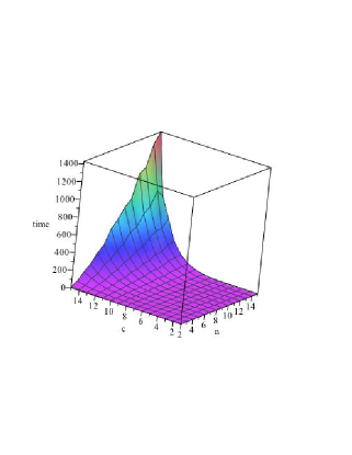
Figure 2: Timings of the special algorithm (Algorithm 1) and the general algorithm

Figure 3: $time$ – $\left(n,c\right)$ of Algorithm 1

(0,0)(6.5,5.5) xunit=0.7cm, yunit=0.25cm -¿(0,0)(8,20) [linecolor=red] (1.466,20)(1.500000000,18.05768355)(1.666666667,9.665910225)(2.,3.744480221)(2.166666667,2.932798584) (2.333333333,2.437350705)(2.500000000,2.110124257) (2.666666667,1.881180152)(3.,1.587270600)(3.333333333,1.410689094) (3.500000000,1.347371056)(3.666666667,1.295297690)(4.,1.215318693) (4.333333333,1.157430378)(4.500000000,1.134286871)(4.666666667,1.114123395) (5.,1.080873798)(5.333333333,1.054809369)(5.500000000,1.043850652) (5.666666667,1.034027547)(6.,1.017223224)(6.333333333,1.003474503) (6.500000000,.9975298610)(6.666666667,.9921137624)(7.,.9826470661) (8.,.9623001836) [linecolor=blue](2.22,20)(2.333333333,11.20930220) (2.500000000,6.597539554)(2.666666667,4.656871062)(3.,3.)(3.333333333,2.293286887) (3.500000000,2.078093084)(3.666666667,1.913896624)(4.,1.681792831) (4.333333333,1.527311397)(4.500000000,1.468389912)(4.666666667,1.418270386) (5.,1.337902603)(5.333333333,1.276674600)(5.500000000,1.251333820) (5.666666667,1.228793555)(6.,1.190550789)(6.333333333,1.159469666) (6.500000000,1.146058034)(6.666666667,1.133837830)(7.,1.112436367) (8.,1.065785556) (8.5,0.5)$c$ (0.4,20)$\sigma$ (1.5,20.5)$E_{1}$ (2.3,20.5)$E_{2}$ (1.2,3.7)$\left(1,1\right)$ (2,10.5)$\left(7,4\right)$ (5.3,9.5)$\left(7,3\right)$

(a) $n=3$

(0,0)(6.5,5.5) xunit=0.7cm, yunit=0.25cm -¿(0,0)(8,20) [linecolor=red] (1.556,20)(1.666666667,12.93605411)(2.,4.856380818)(2.333333333,2.929993587) (2.500000000,2.475736091)(2.666666667,2.165598299)(3.,1.777446336) (3.333333333,1.549955990)(3.500000000,1.469453549)(3.666666667,1.403666207) (4.,1.303331342)(4.333333333,1.231195790)(4.500000000,1.202452016) (4.666666667,1.177444366)(5.,1.136253889)(5.333333333,1.103972260) (5.500000000,1.090389846)(5.666666667,1.078204201)(6.,1.057319880)(6.333333333,1.040175681) (6.500000000,1.032739353)(6.666666667,1.025947964) (7.,1.014030122)(8.,.9880894127) [linecolor=blue](3.256,20)(3.333333333,13.90389170)(3.500000000,8.533095579) (3.666666667,6.143099906)(4.,4.)(4.333333333,3.041244558)(4.500000000,2.741510186) (4.666666667,2.509683836)(5.,2.176376408)(5.333333333,1.949962661)(5.500000000,1.862387088) (5.666666667,1.787261012)(6.,1.665366355)(6.333333333,1.571063718) (6.500000000,1.531590050)(6.666666667,1.496223928)(7.,1.435586873)(8.,1.308424694) (8.5,0.5)$c$ (0.4,20)$\sigma$ (1.6,20.5)$E_{1}$ (3.5,20.5)$E_{2}$ (1.4,3.5)$\left(1,1\right)$ (2.5,11.5)$\left(9,5\right)$ (5.3,10.5)$\left(15,4\right)$

(b) $n=4$

(0,0)(6.5,5.5) xunit=0.7cm, yunit=0.25cm -¿(0,0)(8,20) [linecolor=red] (1.62,20)(1.666666667,17.13618679)(2.,5.753282311)(2.333333333,3.297289806)(2.500000000,2.741237120) (2.666666667,2.367818807)(3.,1.908420862)(3.333333333,1.643695348) (3.500000000,1.550871559)(3.666666667,1.475354856)(4.,1.360768448) (4.333333333,1.278810896)(4.500000000,1.246245046)(4.666666667,1.217950485) (5.,1.171413064)(5.333333333,1.134983728)(5.500000000,1.119661922)(5.666666667,1.105915900) (6.,1.082350640)(6.333333333,1.062989328)(6.500000000,1.054583235)(6.666666667,1.046900140) (7.,1.033398914)(8.,1.003874850) [linecolor=blue](4.1,20)(4.333333333,9.291743603) (4.500000000,6.896492427)(4.666666667,5.509178890)(5.,3.992231088) (5.333333333,3.193133784)(5.500000000,2.922977914)(5.666666667,2.706231428) (6.,2.381253453)(6.333333333,2.150356937)(6.500000000,2.058578178)(6.666666667,1.978654786) (7.,1.846462685)(8.,1.587599363) [linecolor=black](4.285,20)(4.333333333,16.75129000)(4.500000000,10.49876136) (4.666666667,7.635401540)(5.,5.)(5.333333333,3.789954345)(5.500000000,3.406079949) (5.666666667,3.106913324)(6.,2.672696154)(6.333333333,2.374400435)(6.500000000,2.258144910) (6.666666667,2.157966502)(7.,1.994419933)(8.,1.681792831) (8.5,0.5)$c$ (0.4,20)$\sigma$ (1.6,20.5)$E_{1}$ (3.8,20.5)$E_{2}$ (4.6,20.5)$E_{3}$ (1.5,3.5)$\left(1,1\right)$ (3.3,6.5)$\left(11,6\right)$ (4.4,12.5)$\left(31,6\right)$ (6.3,9.5)$\left(31,5\right)$

(c) $n=5$

(0,0)(6.5,5.5) xunit=0.7cm, yunit=0.25cm -¿(0,0)(8,20) [linecolor=red](1.68,20)(1.750000000,14.36635692)(1.800000000,11.81021514) (2.,6.526920830)(2.200000000,4.385794998)(2.250000000,4.051022139)(2.333333333,3.597064004) (2.500000000,2.953990159)(2.666666667,2.527503835)(2.750000000,2.365647355)(3.,2.009592415) (3.250000000,1.775589683)(3.333333333,1.714969410)(3.500000000,1.612385445)(3.666666667,1.529216920) (3.750000000,1.493367984)(4.,1.403521897)(4.250000000,1.333807621)(4.333333333,1.313987732)(4.500000000,1.278493529) (4.666666667,1.247690458)(4.750000000,1.233788113)(5.,1.197093307)(5.250000000,1.166575107)(5.333333333,1.157534305) (5.500000000,1.140905560)(5.666666667,1.125990062)(6.,1.100422364)(6.333333333,1.079412045)(6.500000000,1.070286788) (6.666666667,1.061943601)(7.,1.047273175)(8.,1.015117908) [linecolor=blue] (4.65,20)(4.666666667,18.83229414)(4.750000000,14.35980715)(5.,8.341413292)(5.250000000,5.916678570)(5.333333333,5.408308635) (5.500000000,4.634124038)(5.666666667,4.074641371)(6.,3.324829590)(6.333333333,2.849027733) (6.500000000,2.671705041)(6.666666667,2.522415520)(7.,2.285484381)(8.,1.855059988)

[linecolor=black](5.34,20)(5.333333333,19.65985081)(5.500000000,12.47743774) (5.666666667,9.130485136)(6.,6.)(6.333333333,4.539065405)(6.500000000,4.071281527)(6.666666667,3.704952794) (7.,3.170032825)(8.,2.324494781) (8.5,0.5)$c$ (0.4,20)$\sigma$ (1.6,20.5)$E_{1}$ (4.6,20.5)$E_{2}$ (5.6,20.5)$E_{3}$ (1.5,3.5)$\left(1,1\right)$ (4,6.5)$\left(13,7\right)$ (5.3,9.5)$\left(43,7\right)$ (6.6,8.5)$\left(63,6\right)$

(d) $n=6$

(0,0)(7.7,5.5) xunit=0.55cm, yunit=0.25cm -¿(0,0)(11,20) [linecolor=red] (1.685,20)(2.,7.217631630)(2.333333333,3.853521730) (2.500000000,3.133456137)(2.666666667,2.660700943)(3.,2.092575309) (3.333333333,1.772731253)(3.500000000,1.661997649)(3.666666667,1.572474418) (4.,1.437615655)(4.333333333,1.341880063)(4.500000000,1.304001198)(4.666666667,1.271161322) (5.,1.217280511)(5.333333333,1.175201862)(5.500000000,1.157524232)(5.666666667,1.141671934) (6.,1.114504301)(6.333333333,1.092180588)(6.500000000,1.082483786)(6.666666667,1.073616703) (7.,1.058020031)(8.,1.023789020)(9.,1.001672056)(10.,.9867348137)(11.,.9763238359) [linecolor=blue](5.1,20)(5.333333333,10.59524261)(5.500000000,7.983653347) (5.666666667,6.431156556)(6.,4.691963218)(6.333333333,3.754076768) (6.500000000,3.432844705)(6.666666667,3.173379180)(7.,2.781104818) (8.,2.125209579)(9.,1.801466632)(10.,1.611199548)(11.,1.487160306) [linecolor=purple](6.23,20)(6.333333333,15.44277038)(6.500000000,11.07829450)(6.666666667,8.656808972)(7.,6.084720541)(7.333333333,4.755143336) (7.5,4.308434612) (7.666666667,3.950707522)(8.,3.414902375)(8.5,2.882482960)(9.,2.531338080) (10.,2.099814608)(11.,1.846979686) [linecolor=black](6.39,20)(6.500000000,14.46290919)(6.666666667,10.62707361)(7.,7.)(7.333333333,5.288415739)(7.5,4.736866769)(7.666666667,4.303492379)(8.,3.668016173)(8.5,3.052547604)(9.,2.655264456)(10.,2.176376408) (11.,1.900552860) (11.5,0.5)$c$ (0.4,20)$\sigma$ (1.6,20.5)$E_{1}$ (5.2,20.5)$E_{2}$ (6.02,20.5)$E_{3}$ (6.76,20.5)$E_{4}$ (1.5,1.5)$\left(1,1\right)$ (3.3,6.5)$\left(15,8\right)$ (6.7,4.5)$\left(57,8\right)$ (6.8,12.5)$\left(127,8\right)$ (8.7,5.5)$\left(127,7\right)$

(e) $n=7$

(0,0)(6.7,5.5) xunit=0.55cm, yunit=0.25cm -¿(0,0)(11,20) [linecolor=red](1.726,20) (1.750000000,18.80588525)(2.,7.847547601)(2.250000000,4.646205318) (2.333333333,4.079417777)(2.500000000,3.289741116)(2.666666667,2.775644710) (2.750000000,2.582770669)(3.,2.163221300)(3.250000000,1.891333137) (3.333333333,1.821432173)(3.500000000,1.703665496)(3.666666667,1.60868188) (3.750000000,1.567879296)(4.,1.465991139)(5.,1.233889812)(5.333333333,1.189699024) (5.500000000,1.171144344)(5.666666667,1.154509890)(6.,1.126009141)(6.333333333,1.102593805) (6.500000000,1.092422787)(6.666666667,1.083121484)(7.,1.066758241)(7.333333333,1.052882545) (7.500000000,1.046725519)(8.,1.030815000)(8.500000000,1.017995538)(9.,1.007541595)(9.500000000,.9989296509)(10.,.9917737023) (11.,.9807383124) [linecolor=blue](5.446,20)(5.500000000,17.23944525) (5.666666667,11.45604186)(6.,6.891207384)(6.333333333,5.002752569)(6.500000000,4.428142515)(6.666666667,3.988041222) (7.,3.360764010)(7.333333333,2.937306734)(7.500000000,2.773816625)(8.,2.405904364)(8.500000000,2.155256926)(9.,1.974344572)(9.500000000,1.838104328) (10.,1.732114771)(11.,1.578557606) [linecolor=purple](6.946,20)(7.,17.63500970)(7.333333333,9.727549724) (7.500000000,7.977407307)(8.,5.273807085)(8.500000000,4.030882059) (9.,3.324624566)(9.500000000,2.872234232)(10.,2.559121014)(11.,2.156255469) [linecolor=black](7.415,20)(7.500000000,16.45237470)(8.,8.)(8.500000000,5.402702428) (9.,4.166436205)(9.500000000,3.450604423)(10.,2.986528199) (11.,2.424375951) (11.5,0.5)$c$ (0.4,20)$\sigma$ (1.5,20.5)$E_{1}$ (5.4,20.5)$E_{2}$ (6.8,20.5)$E_{3}$ (7.9,20.5)$E_{4}$ (1.5,1.5)$\left(1,1\right)$ (3.3,4.5)$\left(17,9\right)$ (6.9,5.5)$\left(73,9\right)$ (7.6,9.5)$\left(185,9\right)$ (9.7,5.5)$\left(255,8\right)$

(f) $n=8$

Figure 4: $c$–$\sigma$ graphs for $n=3,4,5,6,7,8$

In this section, we measure how much improvement is provided by the special algorithm over the general algorithm. We use the model for simultaneous decision in Example 1 as a benchmark. In order to measure the performance, we first need to fix the implemental details of several steps. We have made the following choices.

1. In Algorithm 2. Lines 2 and 2 , we use the command BorderPolynomial in DISCOVERER [67] to compute the projection of parametric polynomial equations, which is based on triangular decomposition method.

2. In Algorithm 3. Lines 3, 3, 3, 3, 3 and 3, we first cancel the denominators. It is safe due to the condition (3) in Definition 1. Then we use RootFinding[Isolate] in Maple16 to compute the real solutions of polynomial equations and inequations.

In the following, we provide the experimental results in three figures: Figure 3, Figure 3 and Figure 4.

• Figure 3 provides the timing comparison of Algorithm 1 (Section 5) and the general algorithm (Section 3) for $n=2,\ldots,15$ and $c=1,\ldots,15$. The top entries are the timings in seconds for Algorithm 1 and the bottom entries are for the general algorithm. The symbol $\infty$ means the computational time is greater than $1500$ seconds (aborted). Both programs were written in Maple and were executed on an Intel Core i7 processor (2.3GHz CPU, 4 Cores and 8GB total memory).

  Observe that Algorithm 1 performs much faster than the general algorithm for $n\geq 3$. As is pointed out by [66], when $n>5$, it becomes expensive for the general algorithm to compute the Hurwitz determinants and the sizes of these determinants are usually huge, which leads to much difficulties of the subsequent computations. Moreover, when $c$ is relatively large, the real solution isolation of the general algorithm performs quite slowly, even needs thousands of seconds for one sample point.

  Note also that the special algorithm is a bit slower than the general algorithm when $n=2$. The main reasons are that the special algorithm benefit little from exploiting the special structure and that the special algorithm pays the overhead cost for analyzing the structure.

• Figure 3 provides the timings of Algorithm 1 as a graph over $time$ and $(n,c)$. By fitting, we find that it is very close to the graph of

  $$time\approx 0.012\left(n-2\right)e^{0.6c}.$$

  Observe that the computational time is approximately linear with respect to $n$ (the number of proteins ) and exponential with respect to $c$ (the cooperativity).

• Figure 4 provides, for $n=3,\ldots,8$, the partition of the $c$-$\sigma$ plane into several cells by several curves $E_{i}(c,\sigma)=0$. In each cell, the number of (stable) equilibriums is uniform (presented in each cell). Note that Algorithm 1 can be applied to rational $c$ values. For each $n$, we computed all the critical $\sigma$ values for different rational $c$ values, obtaining sufficiently many $(c,\sigma)$ points. Then we obtained $E_{i}$ by curve fitting.

  Note that we are showing a complete answer to the multistability problem of the system for the given $n$ values. We also remark that the curve $E_{\lceil\frac{n}{2}\rceil}(c,\sigma)=0$ matches $c-n+1-\left(\frac{c}{\sigma}\right)^{\frac{c}{c+1}}=0.$ Note that only when $(c,\sigma)$ is beyond the curve, the number of stable equilibriums is $n$. Thus we have verified the following conjecture in [22] for $n=3,\ldots,8$: the system has exactly $n$ stable equilibriums if and only if $c-n+1-\left(\frac{c}{\sigma}\right)^{\frac{c}{c+1}}>0$.

From the computational results, one sees immediately that the equilibrium classifications of MSRS also have certain special structures, with interesting biological implications. A detailed analysis of the structures and their biological implications will be reported in a forthcoming article.

References

• [1] Anai, H., Yanami, H., 2003. SyNRAC: A maple-package for solving real algebraic constraints. Computational Science ICCS. Springer Berlin Heidelberg, 828–837.
• [2] Anai, H., Weispfenning, V., 2001. Reach Set Computations Using Real Quantifier Elimination, Springer Berlin Heidelberg.
• [3] Arnon, D. S., Dennis, S., 1998. A cluster-based cylindrical algebraic decomposition algorithm. J. Symb. Comput. 5 (1), 189–212.
• [4] Arnon, D. S., Collins, G. E., McCallum, S., 1988. An adjacency algorithm for cylindrical algebraic decompositions of three-dimenslonal space. J. Symb. Comput. 5 (1), 163–187.
• [5] Arnon, D. S., Mignotte, M., 1988. On mechanical quantifier elimination for elementary algebra and geometry. J. Symb. Comput. 5 (1), 237–259.
• [6] Bank, B., Giusti, M., Heintz, J., Pardo, L.-M., 2004. Generalized polar varieties and efficient real elimination procedure. Kybernetika. 40 (5), 519–550.
• [7] Basu, S., Pollack, R., Roy, M.-F., 1996. On the combinatorial and algebraic complexity of quantifier elimination. Journal of ACM. 43 (6), 1002–1045.
• [8] Basu, S., Pollack, R., Roy, M.-F., 1999. Computing roadmaps of semi-algebraic sets on a variety. Journal of the AMS. 3 (1), 55–82.
• [9] Basu, S., Pollack, R., Roy, M.-F., 2006. Algorithms in Real Algebraic Geometry, Springer-Verlag.
• [10] Bradford, R., Davenport, J. H., England, M., McCallum, S., Wilson, D., 2013. Cylindrical Algebraic Decompositions for Boolean Combinations. In: Proceedings of the International Symposium on Symbolic and Algebraic Computation. ACM, 125–132.
• [11] Brown, C. W., 2001. Improved projection for cylindrical algebraic decomposition. J. Symb. Comput. 32 (5), 447–465.
• [12] Brown, C. W., 2001. Simple CAD construction and its applications. J. Symb. Comput. 31 (5), 521–547.
• [13] Brown, C. W., 2003. QEPCAD B: a program for computing with semi-algebraic sets using CADs. ACM SIGSAM Bulletin. 37 (4), 97–108.
• [14] Brown, C. W., 2012. Fast simplifications for Tarski formulas based on monomial inequalities. J. Symb. Comput. 47 (7), 859–882.
• [15] Brown, C. W., 2013. Constructing a single open cell in a cylindrical algebraic decomposition. In: Proceedings of the International Symposium on Symbolic and Algebraic Computation. ACM, 133–140.
• [16] Brown, C. W., McCallum, S., 2005. On using bi-equational constraints in CAD construction. In: Proceedings of the International Symposium on Symbolic and Algebraic Computation. ACM, 76–83.
• [17] Brown, C. W., Novotni, D., Weber, A., 2006. Algorithmic methods for investigating equilibrium in epidemic modeling. J. Symb. Comput. 41 (11), 1157–1173.
• [18] Collins, G. E., 1975. Quantifier Elimination for the Elementary Theory of Real Closed Fields by Cylindrical Algebraic Decomposition. Lecture Notes In Computer Science, Springer-Verlag, Berlin, 33, 134–183.
• [19] Collins, G. E., 1998. Quantifier Elimination and Cylindrical Algebraic Decomposition. Texts and Monographs in Symbolic Computation. Springer-Verlag, Ch. Quantifier elimination by cylindrical algebraic decomposition-20 years of progress.
• [20] Collins, G. E., Hong, H., 1991. Cylindrical algebraic decomposition for quantifier elimination. J. Symb. Comput. 12 (3), 299–328.
• [21] Chen, C., Davenport, J. H., May, J. P., Moreno Maza, M., Xia, B., Xiao, R., 2013. Triangular decomposition of semi-algebraic systems. J. Symb. Comput. 49, 3–26.
• [22] Cinquin, O., Demongeot, J., 2002. Positive and negative feedback: Striking a balance between necessary antagonists. J. Theor. Biol. 216 (2), 229–241.
• [23] Cinquin, O., Demongeot, J., 2005. High-dimensional switches and the modelling of cellular differentiation. J. Theor. Biol. 233 (3), 391–411.
• [24] Cinquin, O., Page, K. M., 2007. Generalized: Switch-like competitive heterodimerization networks. Bulletin of Mathematical Biology. 69 (2), 483–494.
• [25] Davenport, J. H., Heintz, J., 1988. Real quantifier elimination is doubly exponential. J. Symb. Comput. 5 (1), 29–35.
• [26] Dolzmann, A., Seidl, A., Sturm., T., 2004. Efficient projection orders for CAD. In: Proceedings of the International Symposium on Symbolic and Algebraic Computation. ACM, 111–118.
• [27] Dolzmann, A., Sturm, T., 1997. Simplification of quantifier-free formulae over ordered fields. J. Symb. Comput. 24 (2), 209–231.
• [28] Dolzmann, A., Sturm, T., 1997. Redlog: Computer algebra meets computer logic. Acm Sigsam Bulletin. 31 (2), 2–9.
• [29] Dorato, P., Yang, W., Abdallah, C., 1997. Robust multi-objective feedback design by quantifier elimination. J. Symb. Comput. 24 (2), 153–159.
• [30] González-Vega, L., 1996. Applying quantifier elimination to the Birkhoff interpolation problem. J. Symb. Comput. 22 (1), 83–103.
• [31] Grigoriev, D., 1988. Complexity of deciding tarski algebra. J. Symb. Comput. 5 (1-2), 65–108.
• [32] Größlinger, A., Griebl, M., Lengauer, C., 2006. Quantifier elimination in automatic loop parallelization. J. Symb. Comput. 41 (11), 1206–1221.
• [33] Hong, H., 1990. An improvement of the projection operator in cylindrical algebraic decomposition. In: Proceedings of the International Symposium on Symbolic and Algebraic Computation. ACM, 261–264.
• [34] Hong, H., 1990. Improvements in CAD–based Quantifier Elimination. PhD thesis. The Ohio State University.
• [35] Hong, H., 1992. Simple solution formula construction in cylindrical algebraic decomposition based quantifier elimination. In: Proceedings of the International Symposium on Symbolic and Algebraic Computation. ACM, 177–188.
• [36] Hong, H., 1993. Quantifier elimination for formulas constrained by quadratic equations via slope resultants. The Computer Journal. 36 (5), 440–449.
• [37] Hong, H., 1993. Parallelization of quantifier elimination on a workstation network. AAECC-10, LNCS. Springer Verlag, 673, 170–179.
• [38] Hong, H., 1997. Heuristic search and pruning in polynomial constraints satisfaction. Annals of Math. and AI. 19 (3–4), 319–334.
• [39] Hong, H., Liska, R., Steinberg, S., 1997. Testing stability by quantifier elimination. J. Symb. Comput. 24 (2), 161–187.
• [40] Hong, H., Liska, R., Steinberg, S., 1997. Logic, Quantifiers, Computer Algebra and Stability. SIAM News. 30 (6): 10.
• [41] Hong, H., Safey El Din, M., 2009. Variant real quantifier elimination: Algorithm and application. In: Proceedings of the International Symposium on Symbolic and Algebraic Computation. ACM, 183–190.
• [42] Hong, H., Safey El Din, M., 2012. Variant quantifier elimination. J. Symb. Comput. 47 (7), 883–901.
• [43] Jirstrand, M., 1997. Nonlinear control system design by quantifier elimination. J. Symb. Comput. 24 (2), 137–152.
• [44] Lazard, D., 1988. Quantifier elimination: Optimal solution for two classical examples. J. Symb. Comput. 5 (1), 261–266.
• [45] Liska, R., Steinberg, S., 1993. Applying quantifier elimination to stability analysis of difference schemes. Comput. J. 36 (5), 497–503.
• [46] McCallum, S., 1988. An improved projection operation for cylindrical algebraic decomposition of three-dimensional space. J. Symb. Comput. 5 (1), 141–161.
• [47] McCallum, S., 1999. On projection in CAD-Based quantifier elimination with equational constraints. In: Proceedings of the International Symposium on Symbolic and Algebraic Computation. ACM, 145–149.
• [48] McCallum, S., 2001. On propagation of equational constraints in CAD-based quantifier elimination. In: Proceedings of the International Symposium on Symbolic and Algebraic Computation. ACM, 223–230.
• [49] McCallum, S., Collins, G. E., 2002. Local box adjacency algorithms for cylindrical algebraic decompositions. J. Symb. Comput. 33 (3), 321–342.
• [50] Renegar, J., 1992. On the computational complexity and geometry of the first-order theory of the reals. Part I: Introduction. Preliminaries. The geometry of semi-algebraic sets. The decision problem for the existential theory of the reals. J. Symb. Comput. 13 (3), 255–299.
• [51] Renegar, J., 1992. On the computational complexity and geometry of the first-order theory of the reals. Part II: The general decision problem. Preliminaries for quantifier elimination. J. Symb. Comput. 13 (3), 301–327.
• [52] Renegar, J., 1992. On the computational complexity and geometry of the first-order theory of the reals. Part III: quantifier elimination. J. Symb. Comput. 13 (3), 329–352.
• [53] She, Z., Li, H., Xue, B., Zheng, Z., Xia, B., 2013. Discovering polynomial Lyapunov functions for continuous dynamical systems. J. Symb. Comput. 58, 41–63.
• [54] She, Z., Xia, B., Xiao, R., Zheng, Z., 2009. A semi-algebraic approach for asymptotic stability analysis. Nonlinear Analysis: Hybird Systems. 3 (4), 588–596.
• [55] Strzeboński, A., W., 2000. Solving algebraic inequalities. The Mathematica Journal. 7(4), 525–541.
• [56] Strzeboński, A., W., 2005. Applications of algorithms for solving equations and inequalities in Mathematica. In: Algorithmic Algebra and Logic, 243–247.
• [57] Strzeboński, A. W., 2006. Cylindrical algebraic decomposition using validated numeratorics. J. Symb. Comput. 41 (9), 1021–1038.
• [58] Strzeboński, A. W., 2011. Cylindrical decomposition for systems transcendental in the first variable. J. Symb. Comput. 46 (11), 1284–1290.
• [59] Sturm, T., Weber, A., Abdel-Rahman, E. O., Kahoui, M. E., 2009. Investigating algebraic and logical algorithms to solve hopf bifurcation problems in algebraic biology. Mathematics in Computer Science. 2 (3), 493–515.
• [60] Subramani, K., Desovski, D., 2005. Out of order quantifier elimination for Standard Quantified Linear Programs. J. Symb. Comput. 40 (6), 1383–1396.
• [61] Tarski, A., 1951. A Decision Method for Elementary Algebra and Geometry. University of California Press.
• [62] Wang, D., Xia, B., 2005. Stability analysis of biological systems with real solution classification. In: Proceedings of the International Symposium on Symbolic and Algebraic Computation. ACM, 354–361.
• [63] Wang, D., Xia, B., 2005. Algebraic analysis of stability for some biological systems. In: Proceedings of the First International Conference on Algebraic Biology. Universal Academy Press, 75–83.
• [64] Weispfenning, V., 1997. Simulation and optimization by quantifier elimination. J. Symb. Comput. 24 (2), 189–208.
• [65] Niu, W., Wang, D., 2008. Algebraic approaches to stability analysis of biological systems. Math. Comput. Sci. 1 (3), 507–539.
• [66] Niu, W., 2012. Qualitative Analysis of Biological Systems Using Algebraic Methods. PhD thesis. Université Pierre et Marie Curie.
• [67] Xia, B., 2007. DISCOVERER: a tool for solving semi-algebraic systems. ACM Commun. Comput. Algebra. 41 (3), 102–103.
• [68] Xia, B., Yang L., Zhan, N., 2008. Program verification by reduction to semi-algebraic systems solving. Leveraging Applications of Formal Methods, Verification Communications in Computer and Information Science. 17, 277–291.
• [69] Yang, L., Hou, X., Xia, B., 2001. A complete algorithm for automated discovering of a class of inequality-type theorems. Sci. China F: Information Science. 44 (6), 33–49.
• [70] Yang, L., Xia, B., 2008. Automated Proving and Discovering Inequalities (in Chinese). Beijing, Science Press.
• [71] Ying, J. Q., Xu, L., Lin, Z., 1999. A computational method for eetermining strong stabilizability of $n$-D systems. J. Symb. Comput. 27 (5), 479–499.