Star Formation Rate Indicators in WISE/SDSS

Abstract

With the goal of investigating the degree to which the total infrared luminosity ($L_{\rm TIR}$) traces the star formation rate (SFR), we analyze the $L_{\rm TIR}$ from the dust in a sample of $\sim$ 6000 star-forming galaxies, based on the 3.4, 4.6, 12 and 22 $\mu$m data from the Wide-field Infrared Survey Explorer (WISE) and u, g, r, i, z band data from SDSS DR9. These star-forming galaxies are selected by matching the WISE All Sky Catalog with the star-forming galaxy catalog in SDSS DR9 provided by JHU/MPA. The values of $L_{\rm TIR}$ and SFR are derived from the project Code Investigating Galaxy Emission (CIGALE). We study the relationship between the $L_{\rm TIR}$ and SFR. From this study, we derive reference SFR indicators for use in our analysis. Linear correlations between SFR and the $L_{\rm TIR}$ are found, and calibrations of SFRs based on it are proposed. The calibration holds for galaxies with verified observations and agrees well with previous works. The dispersion in the relation between $L_{\rm TIR}$ and SFR could partly be explained by the galaxy’s properties, such as the 4000 Å break.

1 INTRODUCTION

The star formation rate (SFR) is a crucial parameter to characterize the star formation history of galaxies. To calculate the SFR reliably, extensive efforts have been made to derive SFR indicators at various wavelengths, including radio, infrared (IR), ultraviolet (UV), optical spectral lines and continuum (Kennicutt 1998).

UV SFR indicators can directly probes the bulk of the emission from young, massive stars, which make it as a good SFR tracer, while it is highly sensitive to dust reddening and attenuation whose correction techniques depends on the nature of the galaxy ( Buat et al. 2002, 2005, Salim et al. 2007). The optical and NIR SFR indicators, such as hydrogen recombination lines (H$\alpha$,H$\beta$) and forbidden line emission ([O ii], [O iii]) are also good tracers of the ionizing photons from young, massive stars, while it is affected by not only dust extinction though to a much lesser degree than the UV, but also impacted by assumptions on the underlying stellar absorption and on the form of the high end of the stellar initial mass function(Kong et al. 2004; Calzetti et al. 2005). Infrared SFR indicators can be complementary to UV and optical indicators because they measure star formation via the dust-absorbed stellar light that emerges beyond a few $\mu$m(da Cunha et al. 2008). As a result, SFR indicators in the infrared (IR) band have attracted more attention in recent years because of the data with high sensitivity and high angular resolution provided by the Spitzer Space Telescope. As a result, the general correlation between infrared luminosity and SFR has been found and calibrated (Calzetti et al. 2007, 2009, 2010, AlonsoHerrero et al. 2006, Moustakasal et al. 2006, Schmitt et al. 2006, Kennicutt et al. 2007, Persic et al. 2007, Rosa et al. 2007, Bigiel et al. 2008, Rieke et al. 2009).

The monochromatic (i.e., one band or wavelength) infrared SFR diagnostics using Spitzer IRAC detections at 8$\mu$m, Spitzer MIPS detections at 24$\mu$m, 70$\mu$m, 160$\mu$m removes the need for highly uncertain extrapolations of the dust spectral energy distribution across the full wavelength range while it suffers losing most of information in the UV-optical-IR wavelength range (Calzetti et al.2010, Rujopakarn et al.2013).

During the last twenty years, many calibrations of these correlations have focused on the relation between the total luminosity in the IR band ($L_{\rm TIR}$) and SFR because of dust heating in the wide IR band. Calculation of $L_{\rm TIR}$ requires models describing the infrared spectral energy distribution (SED) of star-forming galaxies (Chary & Elbaz 2001, Dale & Helou 2002, Lagache et al.2003, Marcillac et al.2006), but these calibrations usually suffer from small sample size for galaxies and limited sensitivities from surveys such as the Infrared Astronomical Satellite (IRAS) and Infrared Space Observatory (ISO).

The Sloan Digital Sky Survey (SDSS) is the most ambitious imaging and spectroscopic survey to date, and have covered 14,555 square degrees of the sky in the ninth SDSS Data Release. The large area coverage and moderately deep survey limit of the SDSS make it suitable to study the large-scale structure and the characteristics of the galaxy evolution(York et al. 2000).

The Wide-field Infrared Survey Explorer (WISE, Wright et al. 2010) has mapped the entire sky with 5 $\sigma$ point source sensitivities better than 0.08, 0.11, 1 and 6 mJy in bands centered on wavelengths of 3.4, 4.6, 12 and 22 $\mu$m respectively, which is much more sensitive than previous surveys (Cutri et al. 2012). For example, WISE is achieving 100 times better sensitivity than IRAS in the 12 $\mu$m band. As an all-sky survey, WISE has returned data for over 9.4 billion objects, so together with SDSS, WISE provides us with a large sample of star-forming galaxies having reliable photometric flux measurements. The improved sensitivity and large sample size make it suitable for studying the evolution of galaxies.

Start from building a star-forming sample with multi-wavelength observation flux, we derive the SFR for each galaxy by the spectral energy distribution (SED) fitting. $L_{\rm TIR}$ were correlated with the SFR to built the SFR calibrations. This paper is organized as follows. Based on the WISE All Sky Data Release, we present a sample to derive our SFR index calibration (Sect. 2). In Sect. 3, we study the correlation between SFR and the $L_{\rm TIR}$ and perform the numerical calibration. In Sect. 4, we summarize the calibration result and conclude this paper. Throughout the paper, we adopt cosmological parameters of the $\Omega_{M}$ = 0.27 and $\Omega_{\Lambda}$ = 0.73.

2 Data sample selection

To calibrate the relation between $L_{\rm TIR}$ and SFR, we have to first generate a sample from a catalog of sources that have good detections from the WISE All Sky Survey. All the objects in the sample must have reliable flux measurement and therefore reliable calculation of SFR and $L_{\rm TIR}$. For this purpose, we set the selection criteria as follows.

1. The source must have a valid detection and the detection must have a signal to noise ratio $(SNR)>5$ for 3.4, 4.6, 12 and 22 $\mu$m bands.

2. In order to eliminate spurious detections in low coverage areas within Atlas Tiles, such as cosmic ray strikes, residual satellite trails, hot pixel events and scattered light from very bright moving objects such as the moon and planets, we require a reliable band detection which must have been extracted from a region with at least five independent frames image and at least two of the frame image must have been detected with $SNR>3$.

3. In order to eliminate entries that may have incorrect aperture photometry in the largest measurement aperture, which has a radius of 50”, we require the distance to an Atlas Image boundary in the range of between 36.4 and 4058.6 because Atlas Images are 4095x4095 pixels in size and the coadd pixel scale is 1.375”/pix.

4. Filter out spurious detections of image artifacts caused by bright sources.

5. We are only interested in extragalactic galaxies, so we exclude galactic latitudes between -10.0 degrees and 10.0 degrees which are dense with stars in the Milky Way.

6. A variable source is not allowed in our selected galaxy sample by requiring the variability flag($var_{flg}$) that is related to the probability of that the source is variable in that band, to be values of ”0” through ”4” .

7. Ultra-luminous galaxies beyond $z\sim 0.1$ have very different properties compared to the low-redshift star-forming galaxies and hence removed from our sample(Rujopakarn et al.2013).

After compiling a catalog of sources that have good detections from the WISE All-sky Survey, we match this catalog with the catalog of star-forming galaxies in SDSS DR 9 provided by MPA which made use of the spectral diagnostic diagrams from Kauffmann et al. (2003) to classify galaxies as starburst galaxies, active galactic nuclei (AGN), or unclassified. A star-forming galaxy is selected by requiring arc distances between the galaxy identified in SDSS and WISE Catalog to be less than the 6.1” which is the angular resolution of 3.4 $\mu$m bands.

In total, 5,930 star-forming galaxies are adopted in our sample and no multiple matches are found. We use the photometric redshifts provided by SDSS DR9. The flux of WISE in 3.4, 4.6, 12 and 22 $\mu$m bands is aperture curve-of-growth corrected and measured in an circular aperture centered on the source position on the Atlas Image. The flux of SDSS in u, g, r, i, z band is aperture corrected by taking the best fit exponential and de Vaucouleurs fits in each band and asks for the linear combination of the two that best fits the image. The estimation of k-corrections for the photometry observations is not necessary because the redshifts of the galaxies in the sample is restricted to be less than 0.1.

3 Calculation of Star Formation Rate and $L_{\rm TIR}$

An efficient way to derive physical parameters of star formation homogeneously is to fit the observed SED with models from a stellar population synthesis code. We use the SED fitting program package CIGALE (Code Investigating Galaxy Emission, Noll et al. 2009 and Serra et al. 2011) to derive $L_{\rm TIR}$ and SFR. CIGALE was developed to derive highly reliable galaxy properties by fitting the UV-to-far-IR SED and the related dust emission at the same time, i.e., the stellar population synthesized models are connected with infrared templates by the balance of the energy of dust emission and absorption. We refer the reader to Noll et al. (2009) for a detailed description.

For CIGALE, all the light from stars is assumed to be absorbed by dust, and re-emitted in the IR(Buat et al. 2011). SFR is the instantaneous SFR, defined as $(1-f_{ySP})*SFR_{1}+f_{ySP}*SFR_{2}$, where $f_{ySP}$ is the burst strengths(mass fraction of young stellar population), $SFR_{1}$ and $SFR_{2}$ correspond to the star formation rates of the old and young stellar populations, respectively.

Firstly, we combine the redshift-dependent filter fluxes of the 3.4, 4.6, 12 and 22 $\mu$m data from WISE and model flux from SDSS DR9 for our sample, which having been aperture corrected.

Secondly, we apply different scenarios for young and old populations in the same way as in Buat et al. (2011). The input star formation history (SFH) here is a constant burst SFH for young stellar populations, and an exponentially decreasing one for old stellar populations. The stellar population synthesis models of Maraston (2005) are adopted in CIGALE, which include a full treatment of the thermally pulsating asymptotic giant branch (TP-AGB) stars. A Salpeter IMF is used to calculate the complex stellar populations and the stellar metallicity is taken to be solar.

Thirdly, we choose the attenuation curve, which is based on a law given by Calzetti et al. (2000), with modification of the slope and/or by adding a UV bump. The modification of the slope is controlled by the factor $(\lambda/\lambda_{V})^{\delta}$, where $\lambda_{V}$ = 5500 ${\AA}$ is the reference wavelength of the V filter, and $\delta$ is the slope of the attenuation curve. We only considered a modification of the slope for the attenuation law here, and no UV bump was introduced because there is no clear evidence of the presence of such a UV bump for the local galaxies (Buat et al. 2011, and reference therein). We consider different effects of attenuation for old and young stellar populations by adding the reduction factor $f_{\rm att}$ of V-band attenuation for old stellar population(relative to the young one), describing dust attenuation for the old stellar populations.

Fourthly, we choose IR power-law slope $\alpha$, which relates the dust mass to heating intensity. The parameter $\alpha$ is in the interval [1 ;2.5] to cover the main domain of activity.

Finally, depending on the $\chi^{2}$ for the best-fitting models with a set of bins in the parameter space, probability distributions as a function of the parameter value are calculated and used to derive weighted galaxy properties, such as $L_{\rm TIR}$ and instantaneous SFR. The input parameters listed in Table 1 have been demonstrated to be able to obtain a stable and reliable output.

Parameters	Symbol	Range
Star formation history
metallicities (solar metallicity)	$Z$	0.02
$\tau$ of old stellar population models in Gyr	$\tau_{1}$	0.1; 1.0; 10.0
ages of old stellar population models in Gyr	$t_{1}$	2.0;5
ages of young stellar population models in Gyr	$t_{2}$	0.05;0.2
fraction of young stellar population	$f_{ySP}$	0.001; 0.01; 0.1; 0.999
IMF	S	Salpeter
Dust attenuation
Slope correction of the Calzetti law	$\delta$	-0.2; -0.1; 0.0; 0.1; 0.2
V-band attenuation for the young stellar population	$A_{V,ySP}$	0.15; 0.3; 0.45; 0.60; 0.75 ;0.90 ;1.05 ;
		1.20;1.35;1.50;1.65;1.80;1.95;2.1
Reduction of $A_{V}$ based on the old SP model	$f_{\rm att}$	0.50;1.0
IR SED
IR power-law slope	$\alpha$	1.0; 1.5; 2.0; 2.5

Table 1. : List of the input parameters of the code CIGALE and their selected values (see Noll et al. 2009, for detail of parameters description).

4 The reliability of the SED fitting

For a SED fitting, the accuracy of the output relies on the input parameters. To give proper physical parameters, such as SFR, the robustness of the results must be tested. A straightforward method to check the reliability of the output of CIGALE is to compare with comprehensively known physical parameters.

In Fig. 1, we plot the difference in mJy between the flux from the best model estimated by CIGALE and the observed flux for each broad band filter of W1, W2, W3 and W4. It shows that fluxes from the observation are well reproduced by the code, though there is large dispersion. The typical error of model flux increase with the wavelength from W1 to W4 induced by the increasing photometric sensitivity from W1 to W4(Cutri et al. 2012).

There is a cloud of points in large flux region for W1 and W2 that the model flux remain nearly unchanged for the cloud of points in large flux region for W1 and W2. This behaviour indicates the less fit quality for these three filters which is caused by relatively high uncertainties in the object photometry. The relatively bright massive galaxies show greater discrepancies than dim ones, indicating the PSF photometry is less reliable for brighter galaxies, because a considerable part of their flux is left out by the relatively small beam size.

Fig. 1.—: Comparison between the logarithmic flux from the best model estimated by CIGALE and the observed logarithmic flux from each broad band filter of W1, W2, W3 and W4.

Though the code is able to well reproduce the observed data, we cannot be content with this result because it is possible that some SEDs derived by CIGALE are degenerate and correspond to different parameter values. We have to compare each parameter with its Bayesian estimation by the code and the estimation by MPA. We only present the result of SFRs because in this work the SFR is the only parameter in which we are interested.

In Fig. 2, we compare the SFR from MPA($SFR_{mpa}$) and the instantaneous SFR from CIGALE($SFR_{m}$) for our data sample. $SFR_{mpa}$ are estimated using the galaxy photometry following Salim et al. (2007). It shows that SFR values derived by MPA are 0.3 dex larger than the instantaneous SFR from CIGALE($SFR_{m}$) for our data sample below log($SFR_{m}$)=2, and there is a significant dispersion between them. The dispersion between $SFR_{m}$ and $SFR_{mpa}$ could be caused by an insufficient consideration of thermally pulsating asymptotic giant branch (TP-AGB) stars in older but widespread models of Bruzual & Charlot (2003) and Fioc & Rocca-Volmerange (1997; PEGASE), which were used to derive $SFR_{mpa}$ (Brinchmann et al. 2004). As a result, it typically increases the stellar mass by 0.2 dex for star-forming galaxies with important star populations that have an intermediate age (Maraston et al. 2006).

This 0.3 dex offset also can be caused by the different choice of prior star formation history distributions between CIGALE and MPA. The choice of prior star formation history in CIGALE is a constant burst SFH for young stellar populations, and an exponentially decreasing one for old stellar populations, while the prior distributions used in MPA are designed to be as flat as possible. Besides that, the choice of star formation timescales in prior star formation history distributions are also different in this work(see Table 1) and in the MPA(Brinchmann et al. 2004). Pacifici et al. 2012 emphasize that the physical parameters, such as $SFR_{mpa}$, highly depend on the choice of appropriate prior star formation history distributions when applying the Bayesian approach to retrieve from observed spectral energy distributions of galaxies.

The cloud of points above log($SFR_{m}$)=2 seems to lie closer to the MPA value. This agreement implies that the star formation timescales over which both SFR are calculated are similar for these most violent star-forming galaxies. Though the star formation history distribution used in MPA are designed to be flat on the whole, it becomes to decline steeply for the high SFR galaxies(Pacifici et al. 2012, their Fig.4c) which is similar to the choice of star formation history of a constant burst SFH for young stellar populations plus an exponentially decreasing one for old stellar populations in this work.

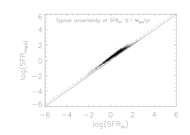
Fig. 2.—: Comparison between SFR from MPA ($SFR_{mpa}$) and the instantaneous SFR from CIGALE ($SFR$) for our data sample. The logarithmic SFR is in units of M${}_{\mbox{${\;{\rm{\hbox{$\odot$}}}}$}}$/yr.

5 Star Formation Rates Calibrator

Star-forming regions tend to be dusty and the cross-section of dust absorption peaks in the UV. Radiation is then reprocessed by dust and emerges beyond a few $\mu$m. As a result, star formation should be closely related to $L_{\rm TIR}$. This knowledge is complicated by the complex physical conditions in the star-forming region. For example, not all of the luminous energy produced by recently formed stars are re-processed by dust in the infrared, which depends on the amount of dust. Secondly, evolved stellar populations also heat the dust, which then emits in the FIR. The other mechanisms are present in Calzetti et al. 2010 and references therein. As a result, it is necessary to check whether the $L_{\rm TIR}$ can be a reliable SFR indicator.

To check whether $L_{\rm TIR}$ values are reliable SFR indicators, In Fig. 3, we show the relation between $L_{\rm TIR}$ and the instantaneous SFR from CIGALE for our data sample. Although there is average 0.5 dex dispersion in the region of $-3.32<log(SFR)<3.07$, all the objects merge into a relatively tight, linear, and steep sequence, which gives strong evidence that the IR luminosities are good SFR indicators.

From the relation between SFR and $L_{\rm TIR}$ for our data sample in Figure 3, we can define a SFR calibration. The observed distribution of all the points in this figure follows a linear least-squares fitting by the expression shown as the dashed line in Fig. 3.

Since both SFR and $L_{\rm TIR}$ are derived from the same fitting procedure, one may wonder whether the relationship is already present in the model library and what is the scatter. We plot the SFR- $L_{\rm TIR}$ relationship in Fig. 4 for all galaxies, not only star-forming galaxies, but also AGN, low S/N LINER, and composite. We make this all galaxies catalog by compiling a catalog of sources that have good detections from the WISE All-sky Survey, and then matching this catalog with the catalog of all galaxies in SDSS DR 9 provided by MPA(Section 2). There is $\sim$23,000 galaxies in total.

It shows that the relation between SFR and $L_{\rm TIR}$ for star-forming sample in Figure 3 is nearly as same as it in Figure 4 for all galaxies. It imply that although the radiation mechanism of AGNs and LINER is different from normal galaxies, AGN and LINER share a SFR - $L_{\rm TIR}$ relation similar to normal star forming galaxy. A possible reason is that the contribution to SED from AGN component and LINER is minor, therefore the host galaxy component dominates the spectrum.

The scatter in Figure 4 is $\sim$ 1.0dex, which is much larger than it in Figure 3. This larger scatter is obviously contributed by AGN activity and LINER.

In the next section, the dispersion in Fig.3 will be discussed.

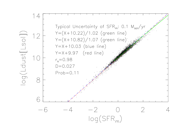
Fig. 3.—: The relation between SFR and $L_{\rm TIR}$ for our data sample. The black dots use the instantaneous SFR from CIGALE($SFR_{m}$). The blue dashed line denotes the best-fit function. The red dot-dashed lines are SFR calibrations from Buat et al. (2008). The green lines are SFR calibrations from Rujopakarn et al.(2013). The logarithmic SFR is in units of M${}_{\mbox{${\;{\rm{\hbox{$\odot$}}}}$}}$/yr. The logarithmic luminosity is in units of L${}_{\mbox{${\;{\rm{\hbox{$\odot$}}}}$}}$. $r_{s}$ is the Spearman’s correlation coefficient of the fit. D is maximum deviation between the cumulative distribution of the data and the fitted function. Prob is the significance level of the two-sided Kolmogorov-Smirnov (K-S) statistic.

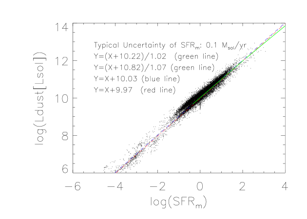
Fig. 4.—: The relation between SFR and $L_{\rm TIR}$ for our data sample. The black dots use the instantaneous SFR from CIGALE($SFR_{m}$). The blue dashed line denotes the best-fit function in Fig.4. The red dot-dashed lines are SFR calibrations from Buat et al. (2008). The green lines are SFR calibrations from Rujopakarn et al.(2013). The logarithmic SFR is in units of M${}_{\mbox{${\;{\rm{\hbox{$\odot$}}}}$}}$/yr. The logarithmic luminosity is in units of L${}_{\mbox{${\;{\rm{\hbox{$\odot$}}}}$}}$.

6 Discussion

6.1 Comparison with other SFR calibrations

In Fig.3, we compare the SFR calibrations from Buat et al. (2008) and Rujopakarn et al.(2013) with ours. The blue dashed line denotes the best-fit function for our work. The red dot-dashed lines are SFR calibrations from Buat et al. (2008). The green lines are SFR calibrations from Rujopakarn et al.(2013) (their Eq.7 and Eq.8, log(SFR) = 1.02log($L_{\rm TIR}$) - 10.22 where $-0.35<log(SFR)<2.11$ and log(SFR) = 1.07log($L_{\rm TIR}$) - 10.82 where $log(SFR)>2.11$). The three calibrations are consistent with each other on the whole besides slight offset.

It shows that SFR values from Buat et al. (2008) are $\sim$0.06 dex larger than ours. The difference could be caused by Buat et al. (2008) assuming that star formation history is a constant SFR over $10^{8}$ years and there is a Kroupa initial mass function ( Kroupa 2001) when making the calibration(their Eq 1), while we use a Salpeter IMF and apply a constant burst SFH for young stellar populations and an exponentially decreasing one for old stellar populations. The use of a Salpeter IMF will cause the SFRs to be smaller by $\sim$0.18 dex than some other IMF with a more shallow slope at low masses (Rieke et al. 2009). Assuming a constant SFR over $10^{8}$ years may not be proper because the star formation process has been proved to be far more complex than a single constant SFR (Kunth et al. 2000).

It shows that SFR calibrations from Rujopakarn et al.(2013) are more consistent with Buat et al. (2008) than our calibration. It can be understood that the calibration of Rujopakarn et al.(2013) is based on the same assumption as Buat et al. (2008) that a continuous star bursts and a Kroupa (2001) IMF.

6.2 The origin of the Dispersion

Although the SFRs are closely related to $L_{\rm TIR}$, the dispersion of the relation is large. To further investigate the dispersion, we plot the relationship between the SFRs and $L_{\rm TIR}$ in Fig.5 for different 4000Å breaks, stellar masses, concentration values and metallicity. To get coincident result, we use the value of 4000Å breaks, stellar masses, concentration values and metallicity from MPA.

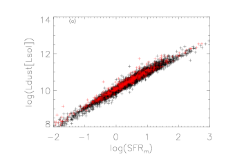
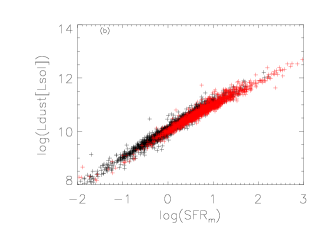
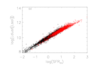
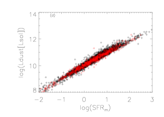
Fig. 5.—: The relation between SFR and $L_{\rm TIR}$ for our data sample. The sample in a) is subdivided into different 4000 Å breaks. Red and black crosses indicate the subsamples with the 4000Å break $>$ 1.2 and 4000Å break $<$ 1.2. The sample in b) is subdivided into different metallicity. Red and black dots indicate the subsamples of $12\,+\,{\rm log(O/H)}$ $>$ 8.9 and $12\,+\,{\rm log(O/H)}$ $<$ 8.9. The sample in c) is subdivided into different stellar masses. Red and black crosses indicate the subsamples of log(stellar mass) $>$ 10.5 and log(stellar mass) $<$ 10.5. The sample in d) is subdivided into different concentration values. Red and black crosses indicate the subsamples of $C>2.6$ and $C<2.6$. The logarithmic luminosity is in units of solar luminosity.

6.2.1 4000Å Break

To show the contribution of the star formation history to the dispersion in the relation between SFR and $L_{\rm TIR}$, we divided the data sample into sub-samples with 4000 Å breaks less than 1.2 and larger than 1.2(Fig. 5a). We choose 1.2 as cut-off point because the star formation density peaks at 4000 Å breaks $\sim$ 1.2(Brinchmann et al.2004). It shows that the $L_{\rm TIR}$-SFR relation at a low 4000 Å break is displaced to higher SFR and lower $L_{\rm TIR}$, especially in the low SFR region. We perform the two-sided Kolmogorov-Smirnov (K-S) statistic test for this case and find that the significance level of the test is 0.14, supporting the idea that the dispersion is partly related to the 4000 Å break.

Brinchmann et al.(2004) show that most of the star formation takes place in galaxies with a low 4000 Å break. This can explain the behavior of the low 4000 Å break displaced to higher SFR, where galaxies with a low 4000 Å break have a younger stellar population, and therefore higher SFR values than high 4000 Å break galaxies with the same SFR. The selection effects also contribute to the effect that galaxies with a high 4000 Å break tend to be excluded from our data sample because these galaxies usually have old stellar populations and seldom show emission lines. If one high 4000 Å break galaxy indeed shows emission lines, it will tend to have less starburst activity, and hence a lower SFR.

6.2.2 Metallicity, Stellar mass and Concentration Index

It is interesting to study whether metallicity of galaxies are related to SFR or not. To investigate this more clearly, we divided the data sample into sub-samples with different metallicity (Fig. 5b). The SFR and $L_{\rm TIR}$ relation at low oxygen abundance is displaced to lower SFR and lower luminosity. We can explain this because the majority of low oxygen abundance galaxies have less star forming events, therefore they have relatively lower SFR. The behavior that the higher oxygen abundance galaxies tends to have higher luminosity (mass) has been studied by many authors (Shi et al. 2005, and references therein ). With the luminosity and metallicity correlation, the most straightforward interpretation is that more massive galaxies form fractionally more stars in a Hubble time (higher luminosity) than low-mass galaxies, and then have higher metallicity. We perform the two-sided Kolmogorov-Smirnov (K-S) statistical test for this case and find that the significance level of the test is 0.

The stellar mass distribution of SDSS galaxies peaks at $logM*\sim 10.5$, so we divided the data sample into sub-samples with $logM*<or>10.5$ in Fig. 5c. It is obvious that the $L_{\rm TIR}$-SFR relation at low stellar mass ($logM*<10.5$ )is displaced to lower SFR and lower luminosity. We can explain it that there is a strong positive correlation between stellar mass and metallicity (Brinchmann et al.2004), so stellar mass should have the same behaviour as metallicity for the $L_{\rm TIR}$-SFR relation. We perform the two-sided Kolmogorov-Smirnov (K-S) statistical test for this case and find that the significance level of the test is 0.

The galaxies with the concentration value $C>2.6$ are mostly early type galaxies whereas late type galaxies have $C<2.6$ . It is well known that early type galaxies are dominated by old/small mass stars, but late type galaxies are dominated by young/massive stars(Kauffmann et al. 2003). In Fig. 5d, we subdivide the sample into sub-samples with different C. It is clear that the concentration value does not contribute to the dispersion. We perform the two-sided Kolmogorov-Smirnov (K-S) statistical test for this case and find that the significance level of the test is 3.2E-5.

7 Conclusions

We have collected a large sample of star-forming galaxies, by matching the WISE data with star forming galaxies catalog of the SDSS DR9. We estimated the global properties of this sample such as the star formation rate, the total infrared luminosity, the stellar mass, the 4000Å break with the code CIGALE which performs a Bayesian analysis to deduce how these parameters are related to the dust attenuation and star formation of each galaxy. Regression analysis was conducted to investigate $L_{\rm TIR}$-SFR relations for this sample. We have confirmed the existence of the correlation between the $L_{\rm TIR}$ and SFR and have obtained a calibration that can be used as a method for determining SFR for star-forming galaxies. The calibration holds for star forming galaxies in the redshift range of less than 0.1, $-3.32<log(SFR)<3.07$, $0.35<log(L_{\rm TIR})<12.7$. The standard Kolmogorov-Smirnov test shows that the dispersion and non-linearity in the relation between $L_{\rm TIR}$ and SFR is partly related to the galaxy’s properties, such as the 4000 Å break.

ACKNOWLEDGMENTS This work was funded by the National Natural Science Foundation of China (NSFC) (Grant Nos. 11203001 and 10873012), the National Basic Research Program of China (973 Program) (Grant No. 2007CB815404), and the Chinese Universities Scientific Fund (CUSF).

This publication makes use of data products from the Wide-field Infrared Survey Explorer, which is a joint project of the University of California, Los Angeles, and the Jet Propulsion Laboratory/California Institute of Technology, funded by the National Aeronautics and Space Administration. Funding for the Sloan Digital Sky Survey (SDSS) has been provided by the Alfred P. Sloan Foundation, the Participating Institutions, the National Aeronautics and Space Administration, the National Science Foundation, the U.S. Department of Energy, the Japanese Monbukagakusho, and the Max Planck Society.

References

- Alonso–Herrero et al. (2006) Alonso–Herrero, A., Rieke, G.H., Rieke, M.J., Colina, L., Perez-Gonzalez, P.G., & Ryder, S.D. 2006, ApJ, 650, 835
- Balogh et al. (1998) Balogh, M. L., Schade, D., Morris, S. L., Yee, H. K. C., Carlberg, R. G., & Ellingson, E. 1998, ApJ, 504, L75
- Buat et al. (2008) Buat, V., Boissier, S., Burgarella, D., et al. 2008, A&A, 483, 107
- Buat et al. (2011) Buat, V., Giovannoli, E., Takeuchi, T. T., et al. 2011, A&A, 529, A22
- Bigiel et al. (2008) Bigiel, F., Leroy, A., Walter, F., Brinks, E., de Blok, W.J.G., Madore, B., Thornley, M.D. 2008, AJ, 136, 2846
- Brinchmann et al. (2004) Brinchmann, J., Charlot, S., White, S. D. M., Tremonti, C., Kauffmann, G., Heckman, T., & Brinkmann, J. 2004, MNRAS, 351, 1151
- Bruzual & Charlot (2003) Bruzual, G., & Charlot, S. 2003, MNRAS, 344, 1000
- Buat et al. (2002) Buat, V., Boselli, A., Gavazzi, G., & Bonfanti, C. 2002, A&A, 383, 801
- Buat et al. (2005) Buat, V., Iglesias-Páramo, J., Seibert, M., et al. 2005, ApJ, 619, L51
- Calzetti et al. (1994) Calzetti, D., Kinney, A. L., & Storchi-Bergmann, T. 1994, ApJ, 429, 582
- Calzetti et al. (2000) Calzetti, D., Armus, L., Bohlin, R. C., Kinney, A. L., Koornneef, J., & Storchi-Bergmann, T. 2000, ApJ, 533, 682
- Calzetti et al. (2005) Calzetti, D., Kennicutt, R.C., Bianchi, L., Thilker, D.A., Dale, D.A., Engelbracht, C.W., Leitherer, C., Meyer, M.J., et al. 2005, ApJ, 633, 871
- Calzetti et al. (2007) Calzetti, D., Kennicutt, R. C., Engelbracht, C. W., et al. 2007, ApJ, 666, 870
- Calzetti et al. (2009) Calzetti, D., & Kennicutt, R. C. 2009, PASP, 121, 937
- Calzetti et al. (2010) Calzetti, D., et al. 2010, ApJ, 714, 1256
- Charlot, S, Fall, S. Michael (2000) Charlot, S, Fall, S. M. 2000, ApJ, 539, 718C
- Chary & Elbaz (2001) Chary, R., & Elbaz, D. 2001, ApJ, 556, 562
- Cutri et al. (2012) Cutri, R. M., Wright, E. L., Conrow, T., et al. 2012, Explanatory Supplement to the WISE All-Sky Data Release Products, 1
- da Cunha et al. (2008) da Cunha, E., Charlot, S., & Elbaz, D. 2008, MNRAS, 388, 1595
- Dale & Helou (2002) Dale, D. A., & Helou, G. 2002, ApJ, 576, 159
- Fioc & Rocca-Volmerange (1997) Fioc, M., & Rocca-Volmerange, B. 1997, A&A, 326, 950
- Kauffmann et al. (2003) Kauffmann, G., et al. 2003, MNRAS, 346, 1055
- Kennicutt (1998) Kennicutt, R. C. 1998, ARA&A, 36, 189
- Kennicutt et al. (2007) Kennicutt, R.C., Calzetti, D., Walter, F., Helou, G.,m Hollenbach, D., Armus, L., Bendo, G., Dale, D.A., Draine, B.T., Engelbracht, C.W., et al. 2007a, ApJ, 671, 333
- Kong (2004) Kong, X. 2004, A&A, 425, 417
- Kroupa (2001) Kroupa, P. 2001, MNRAS, 322, 231
- Kunth Östlin (2000) Kunth, D., Östlin, G. 2000, A&A Rev., 10, 1
- Lagache et al. (2003) Lagache, G., Dole, H., & Puget, J.-L. 2003, MNRAS, 338, 555
- Mann et al. (2002) Mann, R. G., et al. 2002, MNRAS, 332, 549
- Maraston (2005) Maraston, C. 2005, MNRAS, 362, 799
- Maraston et al. (2006) Maraston, C., Daddi, E., Renzini, A., et al. 2006, ApJ, 652, 85
- Marcillac et al. (2006) Marcillac, D., Elbaz, D., Chary, R. R., Dickinson, M., Galliano, F., & Morrison, G. 2006, A&A, 451, 57
- Noll et al. (2009) Noll, S., Burgarella, D., Giovannoli, E., Buat, V., Marcillac, D., & Muñoz-Mateos, J. C. 2009, A&A, 507, 1793
- Nordon et al. (2010) Nordon, R., Lutz, D., Shao, L., et al. 2010, A&A, 518, L24
- Pacifici et al. (2012) Pacifici, C., Charlot, S., Blaizot, J., & Brinchmann, J. 2012, MNRAS, 421, 2002
- Persic & Rephaeli (2007) Persic, M., & Rephaeli, Y. 2007, A&A, 463, 481
- Pilyugin et al. (2004) Pilyugin, L. S., Contini, T., & Vílchez, J. M. 2004, A&A, 423, 427
- Rieke et al. (2009) Rieke, G. H., Alonso-Herrero, A., Weiner, B. J., Pérez-González, P. G., Blaylock, M., Donley, J. L., & Marcillac, D. 2009, ApJ, 692, 556
- Rosa–Gonzalez et al. (2007) Rosa–Gonzalez, D., Burgarella, D., Nandra, K., Kunth, D., Terlevich, E., & Terlevich, R. 2007, MNRAS, 379, 357
- Rujopakarn et al. (2013) Rujopakarn, W., Rieke, G. H., Weiner, B. J., et al. 2013, ApJ, 767, 73
- Salim et al. (2007) Salim, S., et al. 2007, ApJS, 173, 267
- Schmitt et al. (2006) Schmitt, H.R., Calzetti, D., Armus, L., Giavalisco, M., Heckman, T.M., Kennicutt, R.C., Leitherer, C., & Meurer, G.R. 2006, ApJS, 164, 52
- Serra et al. (2011) Serra, P., Amblard, A., Temi, P., et al. 2011, ApJ, 740, 22
- Shi et al. (2005) Shi, F., Kong, X., Li, C., & Cheng, F. Z. 2005, A&A, 437, 849
- Stanghellini et al. (2007) Stanghellini, L., García-Lario, P., García-Hernández, D. A., Perea-Calderón, J. V., Davies, J. E., Manchado, A., Villaver, E., & Shaw, R. A. 2007, ApJ, 671, 1669
- Wright et al. (2010) Wright, E. L., et al. 2010, AJ, 140, 1868
- York et al. (2000) York, D. G., Adelman, J., Anderson, J. E., Jr., et al. 2000, AJ, 120, 1579
- Zheng et al. (2007) Zheng, X. Z., Dole, H., Bell, E. F., Le Floc’h, E., Rieke, G. H., Rix, H.-W., & Schiminovich, D. 2007, ApJ, 670, 301
- Zhu et al. (2008) Zhu, Y.-N., Wu, H., Cao, C., & Li, H.-N. 2008, ApJ, 686, 155