Artificial Neural Network for search for metal poor galaxies

Abstract

Aims. In order to find a fast and reliable method for selecting metal poor galaxies (MPGs), especially in large surveys and huge database, an Artificial Neural Network (ANN) method is applied to a sample of star-forming galaxies from the Sloan Digital Sky Survey (SDSS) data release 9 (DR9) provided by the Max Planck Institute and the Johns Hopkins University (MPA/JHU).

Methods. A two-step approach is adopted:(i) The ANN network must be trained with a subset of objects that are known to be either MPGs or MRGs(Metal Rich galaxies), treating the strong emission line flux measurements as input feature vectors in an n-dimensional space, where n is the number of strong emission line flux ratios. (ii) After the network is trained on a sample of star-forming galaxies, remaining galaxies are classified in the automatic test analysis as either MPGs or MRGs. We consider several random divisions of the data into training and testing sets: for instance, for our sample, a total of 70 per cent of the data are involved in training the algorithm, 15 percent are involved in validating the algorithm and the remaining 15 percent are used for blind testing of the resulting classifier.

Results. For target selection, we have achieved an acquisition rate for MPGs of 96 percent and 92 percent for an MPGs threshold of $12\,+\,{\rm log(O/H)}$=8.00 and $12\,+\,{\rm log(O/H)}$=8.39 , respectively. Running the code takes minutes in most cases under the Matlab 2013a software environment. The code in the paper is available at the web. The ANN method can easily be extended to any MPGs target selection task when the physical property of the target can be expressed as a quantitative variable.

1 Introduction

Extremely metal poor local galaxies are key in an understanding of star formation and enrichment in a nearly pristine interstellar medium (ISM). Metal poor galaxies provide important constraints on the pre-enrichment of the ISM by previous episodes of star formation, e.g by Population III stars (Thuan et al. 2005). Metal poor galaxies are also the best objects for the determination of the primordial He abundance and for constraining cosmological models (e.g. Izotov & Thuan 2004; Izotov et al. 2007). Metal poor galaxies are possibly the closest examples we can find of elementary primordial units from which galaxies formed.

Unfortunately, MPGs are rare. The review by Kunth & Östlin (2000) cites only 31 targets with metallicity below one tenth the solar value. The first extragalactic objects with very low metal abundance were discovered by Searle & Sargent (1972) who reported on the properties of two intriguing galaxies, IZw18 and IIZw40. Their extreme metal under-abundance, more than 10 times less than solar, and even more extreme than that of Hii regions found in the outskirts of spiral galaxies, indicates that these objects could genuinely be young galaxies in the process of formation (Kunth & Östlin 2000). This discovery leads to extensive systematic searches for more objects with low metallicity (see Kunth & Östlin 2000 and references therein) to understand the properties of their massive stars (formation and evolution, appearance of WR stars), the evolution of the dynamics of the gas in the gravitational potential of the parent galaxy as a superbubble evolves, the triggering mechanism that ignites their bursts of star formation, and the chemical enrichment of the interstellar medium after the fresh products are well mixed.

The number of MPGs has significantly increased since the work by Kunth & Östlin (2000), but still the number of known MPGs is small (Morales-Luis et al.2011). The thorough bibliographic compilation described in 4 shows only 421 MPGs with metallicity below two tenth the solar value ( $\hbox{$12\,+\,{\rm log(O/H)}$}<8.0$). There are several reasons that prohibit the identification of more MPGs. One reason is that the MPGs are usually dwarf galaxies which are dim and hard to observe. Another reason is that the methods that determine the metallicity of a galaxy are highly uncertain and there is a large discrepancy between different methods (Shi et al.2005, 2006, 2010).

The metallicity is a key parameter in the search for MPGs. Oxygen is an important element that is easily and reliably determined since the most important ionization stages can be observed. The oxygen abundance from the measurement of electron temperature from [O iii]$\lambda\lambda$4959,5007/[O iii]$\lambda$4363 is one of the most reliable methods, so called the $T_{e}$ method. But [O iii]$\lambda 4363$ is usually weak in low metallicity galaxies, and there are often large errors when measuring this line. In high metallicity galaxies, [O iii]$\lambda 4363$ is hardly even observable.

Instead of the $T_{e}$ method, strong line methods, such as the $R_{23}$ , $P$ , $N2$ , $Ne3O2$ , or $O3N2$ methods, are widely used (Pagel et al. 1979; Kobulnicky, Kennicutt, & Pizagno 1999; Pilyugin et al. 2001; Charlot & Longhetti 2001; Denicoló et al. 2002; Pettini & Pagel 2004; Tremonti et al. 2004; Liang et al. 2006). The $R_{23}$ and $P$ methods suffer the double-valued problem, requiring some assumption or rough a priori knowledge of a galaxy’s metallicity in order to locate it on the appropriate branch of the relation. The $N2$- and $O3N2$ methods are monotonic, but the reasons for this are not purely physical. It is partly due to the N/O ratio increasing on average with the increase in metallicity (Stasińska 2006; Shi et al. 2006). Besides, calibrations of the $O3N2$ and $N2$ indices might be improper for interpreting the integrated spectra of galaxies because $\hbox{[N\,{\sc ii}]}\lambda 6583$ and H$\alpha$ may arise not only in bona fide H ii regions, but also in a diffuse ionized medium. Stasińska (2006) proposed $Ar3O3$ and $S3O3$ as new abundance indicators, which have the advantage of being unaffected by the effects of chemical evolution. The advantages are superior to previous $N2$ and $O3N2$ methods.

In short, the method using a single flux ratio is questionable. The ideal metallicity indicator should use all the strong emission lines. In order to use a method that capitalizes on strong emission lines to identify MPGs, we have employed an automatic Artificial Neural Network(ANN) search for metal poor galaxies in the ninth Sloan Digital Sky Survey data release (SDSS/DR9), by combining all strong emission line flux ratio measurements including $Ne3O2$,[O iii]$\lambda\lambda$4959,5007/[O iii]$\lambda$4363, [O ii]/H$\beta$, [O iii]/H$\beta$, H$\alpha$/H$\beta$, $N2$ and [S ii], provided by MPA. An ANN approach has already successfully been applied to sort out different types of astronomical spectra, from supernovae (Karpenka et al.2013) to quasars (Yèche et al. 2010).

This paper is organized as follows. In Sect. 2, we describe the data set used for training and testing in our analysis, and we present a detailed account of our methodology in Sect. 3. We test the performance of our approach in Sec. 4 by applying to the data and present our results. Finally, we conclude in In Sect. 5. Throughout the paper, we adopt cosmological parameters of the $\Omega_{M}$ = 0.27 and $\Omega_{\Lambda}$ = 0.73.

2 Data sample

In order to use ANN, we must first construct a sample of sources with good emission line detections. All the objects in the sample must have evident and reliable flux ratio measurements, such as $Ne3O2$, [O iii]$\lambda\lambda$4959,5007/[O iii]$\lambda$4363, [O ii]/H$\beta$, [O iii]/H$\beta$, H$\alpha$/H$\beta$, [N ii]/H$\alpha$and [S ii]. For this purpose, we use the catalog of star-forming galaxies in SDSS DR 9 provided by MPA which made use of the spectral diagnostic diagrams from Kauffmann et al. (2003) to classify galaxies as star-forming galaxies, active galactic nuclei (AGN), or unclassified. In total, 84,465 star-forming galaxies are adopted in our sample. All the galaxies in the sample have reliable spectral observations with reasonable values of strong line ratio and oxygen abundance. The redshifts of the galaxies in the sample are in the range of 0.02 $<z<$ 0.3. The oxygen abundance in the sample spans a wide range from 7.1 $<\hbox{$12\,+\,{\rm log(O/H)}$}<$9.5. The distribution of the oxygen abundance in each bin is plotted in Fig.1. It is clearly evident that MPGs are rare compared to metal rich galaxies (MRGs). There are only 8671 galaxies with $\hbox{$12\,+\,{\rm log(O/H)}$}<8.39$($\sim 10$ percent of the star-forming galaxies sample), and among them only 421 galaxies with $\hbox{$12\,+\,{\rm log(O/H)}$}<8.0$($\sim 0.5$ percent of the star-forming galaxies sample).

Figure 1: The distribution of $12\,+\,{\rm log(O/H)}$for our data sample.

3 Artificial Neural Network Approach

The basic building block of the ANN architecture is a processing element called a neuron. The ANN architecture used in this study is illustrated in Fig.2. For target selection, we use an nprtool package developed in the Matlab environment. The nprtool package leads us through solving a pattern-recognition classification problem using a two-layer feed-forward network with sigmoid output neurons. The neuron is the simplest kind of node, and maps an input vector ${\bf x}\in\Re^{n}$ to a scalar output $f({\bf x};{\bf w},\theta)$ via

$$f({\bf x};{\bf w},\theta)=\theta+\sum_{i=1}^{n}{w_{i}x_{i}},$$ (1)

where $\theta$ are ‘bias’ and $\{w_{i}\}$ are ‘weights’ of the i-th variables in the input vector x which include n variables. We will focus mainly on a 2-layer feed-forward ANN, which consists of a hidden layer and an output layer as shown in Fig. 2. The default number of hidden neurons is set to 10. The number of output neurons is set to 2, which is equal to the number of elements in the target vector (MPGs or MRGs).

In order to classify a set of data using an ANN, we need to provide a set of training data (x t). We build the input vector x, that includes redshift, $Ne3O2$, [O iii]$\lambda\lambda$4959,5007/[O iii]$\lambda$4363, $N2$/H$\alpha$,[O iii]/H$\beta$, [S ii], [O ii]/H$\beta$, H$\alpha$/H$\beta$, and [Ar iii]/[O iii]data ( 9 input variables) from the data-set in Section 2. Target t is defined as 0 or 1 to represent MPGs or MRGs. We applied an MPGs cut to $12\,+\,{\rm log(O/H)}$=8.0 (corresponding to 0.2Z_☉), to enhance the selection. Because MPGs are much rarer than MRGs, we select 1,000 MRGs galaxies for $12\,+\,{\rm log(O/H)}$$>$8.0 randomly to avoid systematic errors caused by too many MRGs compared to MPGs.

Then, the input vectors x and target vectors t are randomly divided into three sets as follows: 70 percent are the training set, which is used for computing the gradient and updating the network weights and biases. 15 percent are used to validate that the network is generalizing and to stop training before over-fitting. The last 15 percent are used as a completely independent test of network generalization.

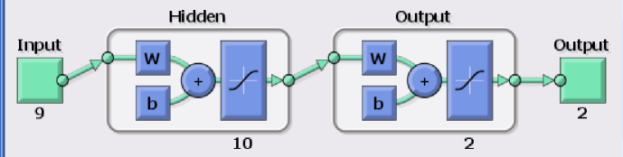
Figure 2: Schematic representation of a 2-layer artificial neural network used here with 9 input variables (redshift, $Ne3O2$, [O iii]$\lambda\lambda$4959,5007/[O iii]$\lambda$4363, $N2$/H$\alpha$,[O iii]/H$\beta$, [S ii], [O ii]/H$\beta$, H$\alpha$/H$\beta$, [Ar iii]/[O iii]) as the input vector x, 10 hidden neurons, and 2 output neurons (MPG or MRGs as target vectors t). This schematic is taken from the MATLAB Recognizing Patterns Documentation.

Once the network weights and biases are initialized, the network is ready for training. The process of training a neural network involves tuning the values of the weights and biases of the network to optimize network performance, as defined by the network performance function. The default performance function for feed-forward networks is mean squared error ($\varepsilon$) between the network outputs f and the target outputs t. It is defined as follows:

$$\varepsilon=\frac{1}{2}\sum_{k}(f_{k}-t_{k})^{2},$$ (2)

Depending on the network architecture, there can be millions of network weights and biases which makes network training a very complicated and computationally challenging task. The nprtool uses the simplest optimization algorithm - gradient descent. It updates the network weights and biases in the direction in which the performance function decreases most rapidly, the negative of the gradient. The gradient will become very small as the training reaches a minimum of the performance. The iteration of this algorithm can be written as

$$x_{k+1}=x_{k}-a_{k}g_{k},$$ (3)

where $x_{k}$ is a vector of current weights and biases, $g_{k}$ is the current gradient, and $a_{k}$ is the learning rate.

4 Spectral selection of MPGs

Once the network has been trained, it is applied to the testing dataset to obtain the predictions for each galaxy therein being either a MPG or a MRG. For illustration, we considered three ANN configurations that differ in terms of the number of variables. The first one uses all variables: redshift, $Ne3O2$, [O iii]$\lambda\lambda$4959,5007/[O iii]$\lambda$4363, $N2$/H$\alpha$,[O iii]/H$\beta$, [S ii], [O ii]/H$\beta$, H$\alpha$/H$\beta$, and [Ar iii]/[O iii]. In the second configuration, We study $T_{e}$ method, strong line methods, such as the $R_{23}$, $Ar3O3$ , $N2$ , $Ne3O2$, or $O3N2$ one by one to show which strong line ratios are most effective in the identification of MPGs. In the third configuration, we plot in Fig.5 the confusion matrices when the MPG threshold is fixed to $12\,+\,{\rm log(O/H)}$=8.39(corresponding to 0.5Z_☉) using all 9 variables to show the changes caused by the MPG threshold. The confusion matrices of configurations are plotted in Figures 3 and 5, respectively. For the introduction to confusion matrices, please see the Matlab Recognizing Patterns web site .

For the first configuration (i.e., using all variables), we achieve an MPG acquisition rate of $\sim$96 percent for MPG threshold of $12\,+\,{\rm log(O/H)}$=8.0. It is therefore apparent that the 9-variable ANN should be used for the purpose of selecting MPGs in any optical spectral catalog. We also plot the Receiver Operating Characteristic (ROC) curves for our analysis procedure in Fig. 4. The ROC curve provides a very reliable way of sorting out the optimal algorithm in signal detection theory. The ROC curve is a plot of the true positive rate (sensitivity) versus the false positive rate (1 - specificity). A perfect test would show points in the upper-left corner, with 100 percent accuracy. One sees in Fig. 4 that nprtool yields very reasonable ROC curves, indicating that the classifiers are quite discriminative.

Figure 3: the confusion matrices for training, testing, and validation, and the three kinds of data combined for setting the MPG threshold to $12\,+\,{\rm log(O/H)}$=8.0 using all 9 variables. The diagonal cells show the number of cases that were correctly classified, and the off-diagonal cells show the misclassified cases. The blue cell in the bottom right shows the total percent of correctly classified cases (in green) and the total percent of misclassified cases (in red).

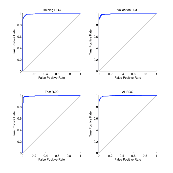
Figure 4: The colored lines in each axis represent Receiver Operating Characteristic (ROC) curve for training, testing and validation, and the three kinds of data are combined for setting the MPG threshold to $12\,+\,{\rm log(O/H)}$=8.0.

For the sencond configuration, we identify MPGs only using the essential information for $T_{e}$-method ( redshift, [O iii]$\lambda\lambda$4959,5007/[O iii]$\lambda$4363, [O iii]/H$\beta$, [S ii], [O ii]/H$\beta$), $R_{23}$-method (redshift, [O iii]/H$\beta$, [O ii]/H$\beta$), $N2$-method(redshift, $N2$/H$\alpha$), $O3N2$-method(redshift, $N2$/H$\alpha$, [O iii]/H$\beta$), $Ne3O2$-method(redshift, [Ne iii]$\lambda 3869$/[O ii]$\lambda 3727$ ) $Ar3O3$- method(redshift, [Ar iii]/[O iii]). We found that the acquisition rate for MPGs reduced by a few percent when using only one method, 92.3$\%$ for the $T_{e}$- method, 90.9$\%$ for the $R_{23}$-method, 96.2$\%$ for the $N2$-method , 96.2$\%$ for the $O3N2$-, 85.8$\%$ for the $Ne3O2$-method and 88.7$\%$ for the $Ar3O3$- method(See Table 1). All the oxygen abundance determination methods based on these strong line ratios are reliable to a certain degree. In any case, it is an essential parameter for redshift to identify MPGs because it is vital to make the accurate redshift correction when deriving the the flux of the strong emission line.

It is impressive that the acquisition rate for MPGs by $N2$-method and $Ne3O2$-method are comparable to it using all 9 variables. It might imply that both $N2$-method and $Ne3O2$-method are monotonic, free of internal reddening correction, and therefore superior to other oxygen abundance determination methods.

We add (H$\alpha$/H$\beta$) line ratio to each method for shown of the influence of internal reddening correction on identifying MPGs. This parameter is probed because the internal reddening correction is a fundamental step for determining $12\,+\,{\rm log(O/H)}$(Shi et al.2005, 2006). We find that the acquisition rate for MPGs increases from 85.8$\%$ to 88.1$\%$ for the $Ne3O2$-method , 90.9$\%$ to 92.5$\%$ for the $R_{23}$-method and 88.7$\%$ to 90.9$\%$ for the $Ar3O3$- method when adding (H$\alpha$/H$\beta$) to them(See Table 1). The acquisition rate for MPGs for the rest three methods( $T_{e}$-, $N2$-, $O3N2$- method) do not change when adding (H$\alpha$/H$\beta$) to them, which can be explained that the uncertainty of the internal reddening correction is comparable to the uncertainty of $T_{e}$-method and [N ii]$\lambda$6583/H$\alpha$$\lambda$6563, [O iii]$\lambda$5007/H$\beta$)/([N ii]$\lambda$6583/H$\alpha$flux ratio is not sensitive the internal reddening correction.

Table 1: The acquisition rate for MPGs as a function of the different variables.

	$T_{e}$	$N2$	$O3N2$	$R_{23}$	$Ne3O2$	$Ar3O3$
Z1	0.923	0.962	0.962	0.909	0.858	0.887
Z+ H$\alpha$/H$\beta$2	0.915	0.960	0.960	0.925	0.881	0.909

1: The strong emission line ratios for each method plus redshift to identify MPGs.
2: The strong emission line ratios for each method plus redshift and (H$\alpha$/H$\beta$) to identify MPGs.

To show the changes in performance caused by the MPG threshold, we plot in Fig.5 the confusion matrices when the MPG threshold is fixed to $12\,+\,{\rm log(O/H)}$=8.39(corresponding to 0.5Z_☉) using all 9 variables: redshift, $Ne3O2$, [O iii]$\lambda\lambda$4959,5007/[O iii]$\lambda$4363, $N2$/H$\alpha$, [O iii]/H$\beta$, [S ii], [O ii]/H$\beta$, H$\alpha$/H$\beta$and [Ar iii]/[O iii]. There are 8671 MPGs when the MPG threshold is fixed to $12\,+\,{\rm log(O/H)}$=8.39 and we select 10,000 MRGs galaxies for $12\,+\,{\rm log(O/H)}$=8.39 randomly to avoid systematic error caused by too many MRGs compared to MPGs. It is shown that the MPGs acquisition rate decreases a few percent compared to the MPG threshold of $12\,+\,{\rm log(O/H)}$=8.0. This may imply that $12\,+\,{\rm log(O/H)}$=8.39 is a less suitable MPG threshold than $12\,+\,{\rm log(O/H)}$=8.00.

Figure 5: The confusion matrices for training, testing, and validation, and the three kinds of data combined for the MPG threshold to $12\,+\,{\rm log(O/H)}$=8.39 using all 9 variables.

5 Conclusions

We have presented a promising new approach to select MPGs from spectral catalogs. It involves the application of an artificial neural network with a 2-layer feed-forward architecture. The input variables are spectral measurements, i.e., redshift and the most observably strong emission line ratios.

In the target selection, we have achieved an MPG acquisition rate of 96 percent and 92 percent for an MPG threshold of $12\,+\,{\rm log(O/H)}$=8.00 and $12\,+\,{\rm log(O/H)}$=8.39, respectively from $\sim$80,000 star forming galaxies. The oxygen abundance of a galaxy in the MPG sample have a 96 percent chance to be lower than $12\,+\,{\rm log(O/H)}$=8.00 for an MPG threshold of $12\,+\,{\rm log(O/H)}$=8.00.

All the oxygen abundance determination methods based on these strong line ratios are reliable to a certain degree, such as the $T_{e}$-, $R_{23}$-, $N2$- , $O3N2$-, $Ne3O2$- method, and so on. The acquisition rate for MPGs by $N2$-method and $O3N2$-method are comparable to it using all 9 variables. It shows serious potential to search new MPGs candidate with a single emission line ratio, such as [N ii]$\lambda$6583/H$\alpha$$\lambda$6563.

This new statistical methods developed in the context of the SDSS project can easily be extended to any other analysis requiring MPG selection when the physical property of the target can be quantitative.

Finally, we note that, aside from its relative simplicity and robustness, the ANN classification method that we have presented here can be extended and improved in a number of ways, such as increase of neuron number, adoption of three-layer network, or making the multi category classification. One have to be cautioned that both the classification accuracy and run-time may change dramatically in these processes.