Scaling relations and mass bias in hydrodynamical $f(R)$ gravity simulations of galaxy clusters

Abstract

We investigate the impact of chameleon-type $f(R)$ gravity models on the properties of galaxy clusters and groups. Our $f(R)$ simulations follow for the first time also the hydrodynamics of the intracluster and intragroup medium. This allows us to assess how $f(R)$ gravity alters the X-ray scaling relations of clusters and how hydrostatic and dynamical mass estimates are biased when modifications of gravity are ignored in their determination. We find that velocity dispersions and ICM temperatures are both increased by up to $1/3$ in $f(R)$ gravity in low-mass haloes, while the difference disappears in massive objects. The mass scale of the transition depends on the background value $f_{R0}$ of the scalar degree of freedom. These changes in temperature and velocity dispersion alter the mass-temperature and X-ray luminosity-temperature scaling relations and bias dynamical and hydrostatic mass estimates that do not explicitly account for modified gravity towards higher values. Recently, a relative enhancement of X-ray compared to weak lensing masses was found by the Planck Collaboration (2013). We demonstrate that an explanation for this offset may be provided by modified gravity and the associated bias effects, which interestingly are of the required size. Finally, we find that the abundance of subhaloes at fixed cluster mass is only weakly affected by $f(R)$ gravity.

1 Introduction

There are essentially two classes of models describing the late time accelerated expansion of the Universe. In the first class, dubbed “dark energy” models, a new component is added to the energy-momentum tensor of general relativity (GR). To drive the observed accelerated expansion, this matter species or field has an equation of state which provides a negative pressure. A prominent example for this type of model is vacuum energy as considered in the standard $\Lambda$ cold dark matter ($\Lambda$CDM) cosmology. In the second class, modifications to general relativistic gravity are introduced that account for the accelerated expansion. One of these so called “modified gravity” models is $f(R)$ gravity, in which a suitable scalar function $f(R)$ is added to the Ricci scalar $R$ in the gravitational part of the action.

Since Einstein’s general relativity is very well tested in the Solar system, modified gravity models need a mechanism which ensures that the modifications of gravity are suppressed locally so that observational constraints are not violated. Several such models with screening mechanisms have been constructed, such as the Chameleon (Khoury & Weltman, 2004), the Symmetron (Hinterbichler & Khoury, 2010), the Dilaton (Gasperini et al., 2002), and the Vainshtein (Vainshtein, 1972; Deffayet et al., 2002) mechanisms. In this work, we explore $f(R)$ gravity models which exhibit a Chameleon-type screening (Hu & Sawicki, 2007). The screening of modified gravity effects is related to large non-linear perturbations in the scalar degree of freedom which appear in this model. More precisely, the screening length below which gravity is significantly affected becomes negligibly small in these large perturbations which are associated with matter over-densities like our Galaxy. Because of these non-linearities, the effects on cosmic structure formation are only accessible through detailed numerical simulations.

Recent numerical works on Chameleon-type $f(R)$ models of modified gravity focused on quantities which can be studied with collisionless simulations. The scale-dependent enhancement of the matter power spectrum (e.g. Oyaizu, 2008; Li et al., 2012, 2013; Puchwein et al., 2013; Llinares et al., 2013) and halo mass function (e.g. Schmidt et al., 2009; Ferraro et al., 2011; Zhao et al., 2011a; Li & Hu, 2011) was analysed, as well as the impact of $f(R)$ gravity on cluster concentrations (Lombriser et al., 2012a) and density profiles (Lombriser et al., 2012b), halo velocity dispersions (Schmidt, 2010; Lombriser et al., 2012a; Lam et al., 2012), redshift-space distortions (Jennings et al., 2012), and the integrated Sachs-Wolfe effect (Cai et al., 2013).

Our modified gravity simulation code, mg-gadget (Puchwein et al. 2013), allows us to follow baryonic physics and modified gravity at the same time. This offers the opportunity to investigate the ICM temperatures, the hydrostatic mass bias, the X-ray luminosities and the thermal Sunyaev–Zeldovich (SZ) signals of galaxy cluster and groups. Here, we assess how $f(R)$ gravity affects these quantities, as well as cluster velocity dispersions, subhalo abundances and dynamical mass estimates.

In Sect. 2, we briefly summarize the main properties of the $f(R)$ gravity model which we consider. An overview of how our modified gravity simulation code works and what runs have been performed with it is provided in Sect. 3. Our results are presented in Sect. 4. We summarize our findings and draw our conclusions in Sect. 5.

2 ${f}(R)$ gravity

$f(R)$ gravity models generalize Einstein’s general relativity by adding a function $f(R)$ to the Ricci scalar $R$ in the gravitational part of the action. The action is then given by

$$S=\int{\rm d}^{4}x\sqrt{-g}\left[\frac{R+f(R)}{16\pi G}+\mathcal{L}_{m}\right],$$ (1)

where $g$ is the determinant of the metric, $G$ is the gravitational constant and $\mathcal{L}_{m}$ is the Lagrangian density of matter. Demanding that the variation of this action with respect to the metric vanishes leads to the modified Einstein equations (Buchdahl, 1970)

$$G_{\mu\nu}+f_{R}R_{\mu\nu}-\left(\frac{f}{2}-\Box f_{R}\right)g_{\mu\nu}-\nabla_{\mu}\nabla_{\nu}f_{R}=8\pi GT_{\mu\nu},$$ (2)

where $G_{\mu\nu}=R_{\mu\nu}-Rg_{\mu\nu}/2$ is the Einstein tensor and $f_{R}\equiv\text{d}f/\text{d}R$. Models which are compatible with observational constraints require $|f_{R}|\ll 1$. On scales much smaller than the horizon, the quasi-static approximation is valid (Oyaizu, 2008; Noller et al., 2014) so that time derivatives can be neglected in the above equation. Together, this allows us to simplify the field equation for $f_{R}$ to (e.g. Oyaizu (2008), also see Appendix A)

$$\nabla^{2}f_{R}=\frac{1}{3}\left(\delta R-8\pi G\delta\rho\right),$$ (3)

where $\delta R$ and $\delta\rho$ denote the perturbations in the scalar curvature and matter density, respectively. Considering Eq. (2) in the Newtonian limit, a modified Poisson equation for the gravitational potential is obtained (Hu & Sawicki 2007, also see Appendix A)

$$\nabla^{2}\Phi=\frac{16\pi G}{3}\delta\rho-\frac{1}{6}\delta R.$$ (4)

In order to follow cosmic structure formation in $f(R)$ models, our code needs to solve the two partial differential equations (3) and (4). The former equation is particularly challenging to solve due to its non-linearity.

However let us first consider our choice of $f(R)$. Since GR is well tested in the Solar system, modified gravity models should show the same behaviour as GR in high density regions, or more precisely in our local environment within the Milky Way. This is achieved in a class of models which exhibit a chameleon mechanism, such as the model proposed by Hu & Sawicki (2007),

$$f(R)=-m^{2}\frac{c_{1}\left(\frac{R}{m^{2}}\right)^{n}}{c_{2}\left(\frac{R}{m^{2}}\right)^{n}+1},$$ (5)

where $m^{2}\equiv H_{0}^{2}\Omega_{m}$. For a suitable choice of the parameters $c_{1}$, $c_{2}$ and $n$, the chameleon mechanism screens $f(R)$ effects in high density regions. By also requiring

$$\frac{c_{1}}{c_{2}}=6\frac{\Omega_{\Lambda}}{\Omega_{m}} c_{2}\left(\frac{R}{m^{2}}\right)^{n}\gg 1,$$ and (6)

an expansion history of the universe is obtained which closely mimics the one inferred with a $\Lambda$CDM cosmological model (see e.g. Hu & Sawicki, 2007). In this scenario, the derivative of $f(R)$ is given by

$$f_{R}=-n\frac{c_{1}\left(\frac{R}{m^{2}}\right)^{n-1}}{\left[c_{2}\left(\frac{R}{m^{2}}\right)^{n}+1\right]^{2}}\approx-n\frac{c_{1}}{c_{2}^{2}}\left(\frac{m^{2}}{R}\right)^{n+1},$$ (7)

where the second equality holds in the assumed limit $c_{2}\left(\frac{R}{m^{2}}\right)^{n}\gg 1$. For a more convenient characterization of a specific $f(R)$ model, the parameter set $c_{1}$ and $c_{2}$ can be replaced by the background value of $f_{R}$ at $z=0$, $\bar{f}_{R0}$, as follows: the background curvature of a Friedmann–Robertson–Walker universe is given by

$$\bar{R}=12H^{2}+6\frac{\text{d}H}{\text{d}\ln a}H,$$ (8)

which translates into

$$\bar{R}=3m^{2}\left[a^{-3}+4\frac{\Omega_{\Lambda}}{\Omega_{m}}\right]$$ (9)

for a flat $\Lambda$CDM expansion history. Plugging this equation for $a=1$ into Eq. (7) and additionally demanding that the first equality in Eq. (6) is satisfied constrains the parameters $c_{1}$ and $c_{2}$ completely for given values of $\Omega_{\Lambda}$, $\Omega_{m}$, $H_{0}$, $\bar{f}_{R0}$ and $n$. Hence, $\bar{f}_{R0}$ and $n$ can be used instead of $c_{1}$, $c_{2}$ and $n$ to completely specify the model. In the following sections, we will therefore describe the considered $f(R)$ models by their value of $\bar{f}_{R0}$. $n$ is fixed to $1$ in the simulations presented in this work.

3 The simulations

Our simulations were carried out with the modified gravity simulation code mg-gadget (Puchwein et al. 2013). The code is an extension and modification of p-gadget3, which is itself based on gadget-2 (Springel 2005). An advantage of using p-gadget3 as a basis for the modified gravity code is that numerical models for a large number of physical processes, such as hydrodynamics, gas cooling, star formation and associated feedback processes are already implemented in this code. It is, hence, possible to follow such baryonic processes and modified gravity at the same time. Especially the possibility to account for hydrodynamics in modified gravity simulations is essential for the analysis carried out in this work.

Here, we provide only a very brief overview of how the mg-gadget code solves the partial differential equations that arise in $f(R)$ gravity. A detailed description of the code functionality and the algorithms that are employed is given in Puchwein et al. (2013). To solve the equation for $f_{R}$, i.e. Eq. (3), the code uses an iterative multigrid-accelerated Newton-Gauss-Seidel relaxation scheme on an adaptively refined mesh. This method is computationally efficient, well suited for very non-linear equations and provides high spatial resolution in high density regions, like in collapsed haloes. Note however, that instead of solving directly for $f_{R}$, the code iteratively computes $u\equiv\ln(f_{R}/\bar{f}_{R}(a))$. This ensures that $f_{R}$ cannot attain unphysical positive values due to the finite step size of the iterative solver, which makes the code numerically more stable (see also Oyaizu, 2008).

Once $f(R)$ is known, the modified Poisson equation (4) can be rewritten as

$$\nabla^{2}\Phi=4\pi G(\delta\rho+\delta\rho_{\rm eff}),$$ (10)

where the effective mass density $\delta\rho_{\rm eff}$ encodes the modified gravity effects and is given by

$$\delta\rho_{\rm eff}=\frac{1}{3}\delta\rho-\frac{1}{24\pi G}\delta R.$$ (11)

Adopting $n=1$, the following expression for $\delta R$ can be obtained from Eq. (7)

$$\delta R=\bar{R}(a)\left(\sqrt{\frac{\bar{f}_{R}(a)}{f_{R}}}-1\right).$$ (12)

Hence, the code can compute the right-hand side of Eq. (10) using the solution for $f(R)$, as well as the true mass density. The resulting Poisson equation is subsequently solved with essentially the same TreePM gravity solver which p-gadget3 uses for standard Newtonian gravity. The hydrodynamics is followed with p-gadget3’s entropy conserving smoothed particle hydrodynamics scheme (Springel & Hernquist, 2002).

In the following, we will analyze four different sets of simulations, each of them consisting of a $\Lambda$CDM and one or more $f(R)$ simulations which, all based on the same initial conditions. The parameters of the simulations and the names by which we refer to them are summarized in Table 1. Three of these sets consist of pure dark matter, or more precisely collisionless simulations, while the fourth set includes non-radiative hydrodynamical runs as well.

Simulation	Box size $($\mathrm{M}\mathrm{p}\mathrm{c}$/h)$	Number of particles	Simulation type	Gravity
DM-small	$100$	$256^{3}$	Collisionless	GR and $|\bar{f}_{R0}|=10^{-5}$
DM-large	$200$	$256^{3}$	Collisionless	GR and $|\bar{f}_{R0}|=10^{-4/5/6}$
DM-high-res	$100$	$512^{3}$	Collisionless	GR and $|\bar{f}_{R0}|=10^{-4}$
Nonrad	$200$	$2\times 256^{3}$	Non-radiative hydro.	GR and $|\bar{f}_{R0}|=10^{-5}$

Table 1: Overview of the simulations we have performed. We will refer to the runs by the names provided in the first column. The box sizes are given in comoving coordinates.

4 Results

4.1 Velocity dispersions of clusters and groups

As a first step in exploring the dynamical properties of our simulated clusters and groups, we have computed the one-dimensional velocity dispersions of the ‘DM-large’ simulation particles within $r_{\rm 200crit}$, which is the radius of a sphere that is centred on the potential minimum of the cluster and inside which the mean density is 200 times the critical density of the Universe. To this end, the haloes have been identified and their potential minima have been found with the subfind code (Springel et al., 2001). The results, which are based on the DM-large simulations, are displayed in Fig. 1 for GR, as well as for$|\bar{f}_{R0}|=10^{-6}$, $10^{-5}$ and $10^{-4}$.

The figure illustrates both the enhancement of the velocity dispersion due to modified gravity effects, as well as their screening in massive haloes. For $|\bar{f}_{R0}|=10^{-4}$ the velocity dispersion is increased by about $1/3$ with respect to $\Lambda$CDM over the whole mass range. In this model, even the gravitational potential wells of clusters are not deep enough for the chameleon mechanism to become fully effective. This increment is, hence, theoretically expected. In particular, combining equations (10) and (11) for $\delta R\approx 0$, i.e. in the low-curvature regime, leads to forces larger by a factor of $4/3$ with respect to GR, which translates into an increase of the squared velocity dispersions by roughly the same factor.

For $|\bar{f}_{R0}|=10^{-5}$, the mass threshold for the onset of the chameleon mechanism is smaller. This is reflected by our results. At low masses, which correspond to more shallow potential wells, the velocity dispersion is again increased by a factor of $\sim 4/3$ compared to $\Lambda$CDM. At about $10^{14}M_{\odot}$ the chameleon mechanism sets in and the difference between $f(R)$ and $\Lambda$CDM decreases until it vanishes almost completely roughly above $10^{14.5}M_{\odot}$.

In the $|\bar{f}_{R0}|=10^{-6}$ cosmology, the $f(R)$ effects on gravity are screened essentially over the whole mass range shown in the figure. Thus, there is almost no difference in the median curves of the $\Lambda$CDM and $f(R)$ runs. A small deviation is, however, present at the low mass end. This presumably indicates the transition to the unscreened low-curvature regime. Overall, these results are in good agreement with the findings of Schmidt (2010).

One can obtain a simple analytic estimate of the velocity dispersion threshold above which the chameleon mechanism screens modified gravity effects. Note that in the low curvature regime $\nabla^{2}f_{R}\approx-\frac{8\pi G}{3c^{2}}\delta\rho\approx-\frac{2}{3c^{2}}\nabla^{2}\phi_{\rm N}$, where $\phi_{\rm N}$ is the Newtonian gravitational potential. From this one finds $\delta f_{R}\approx-\frac{2}{3c^{2}}\phi_{\rm N}$ in the unscreened regime. The chameleon effect becomes effective once strong non-linearities appear. According to Eq. (12), this happens when $|\delta f_{R}|$ approaches $|\bar{f}_{R}|$. Hence, chameleon screening is active for $|\phi_{\rm N}|\gtrsim\frac{3c^{2}}{2}|\bar{f}_{R}|$ (e.g. Hu & Sawicki, 2007; Cabré et al., 2012). For the sake of simplicity we ignore for the moment factors of approximately $\sim\sqrt{(4/3)}$ due to modified gravity effects when translating the Newtonian potential to a three-dimensional halo velocity dispersion $\sigma$. Assuming $\sigma_{\rm 3D}\approx\sqrt{\phi_{\rm N}}$, this results in a threshold value for the onset of chameleon screening of $\sigma_{\rm 3D}\gtrsim\sqrt{\frac{3c^{2}}{2}\bar{f}_{R}}$. Figure 2 displays this quantity as a function of redshift for models with $|\bar{f}_{R0}|=10^{-6}$, $10^{-5}$ and $10^{-4}$.

For $|\bar{f}_{R0}|=10^{-4}$ and $z=0$, the onset of screening is expected at $\sigma_{1\text{D}}=\sigma_{3\text{D}}/\sqrt{3}\approx\sqrt{10^{6.6}}\,{\rm km\,s^{-1}}$, which is even larger than the values found in our most massive simulated galaxy clusters. The theoretical value for $|\bar{f}_{R0}|=10^{-5}$ at $z=0$, i.e. ${\sigma_{1\text{D}}}=\sqrt{10^{5.6}}\,{\rm km\,s^{-1}}$, is in good agreement with the position of the transition region in the simulation. The theoretical value for the onset of screening in the $|\bar{f}_{R0}|=10^{-6}$ cosmology is $\sigma_{1\text{D}}\approx\sqrt{10^{4.6}}\,{\rm km\,s^{-1}}$, which is compatible with the slight increase in the velocity dispersion that we find for low mass objects in the corresponding simulation.

Note, however, that the simple derivation presented above neglects the effects of environment. In particular, the Newtonian gravitational potential is not only affected by an object’s mass but also by its surroundings. Thus, even objects with masses below the derived screening threshold can be screened, if they reside in a high density region. This effect could result in increased scatter of the properties of low mass objects in $f(R)$ gravity. Massive galaxy clusters are in contrast not expected to be strongly affected.

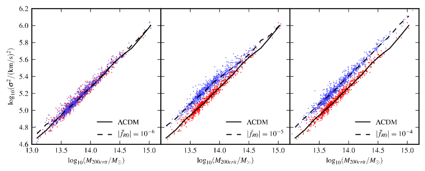
Figure 1: One-dimensional velocity dispersion of the ‘DM-large’ simulation particles as a function of halo mass $M_{\rm 200crit}$ for $\Lambda$CDM (red dots, solid line) and $f(R)$ (blue dots, dashed line) cosmologies and different $\bar{f}_{R0}$ values. Lines show the medians of the binned data.

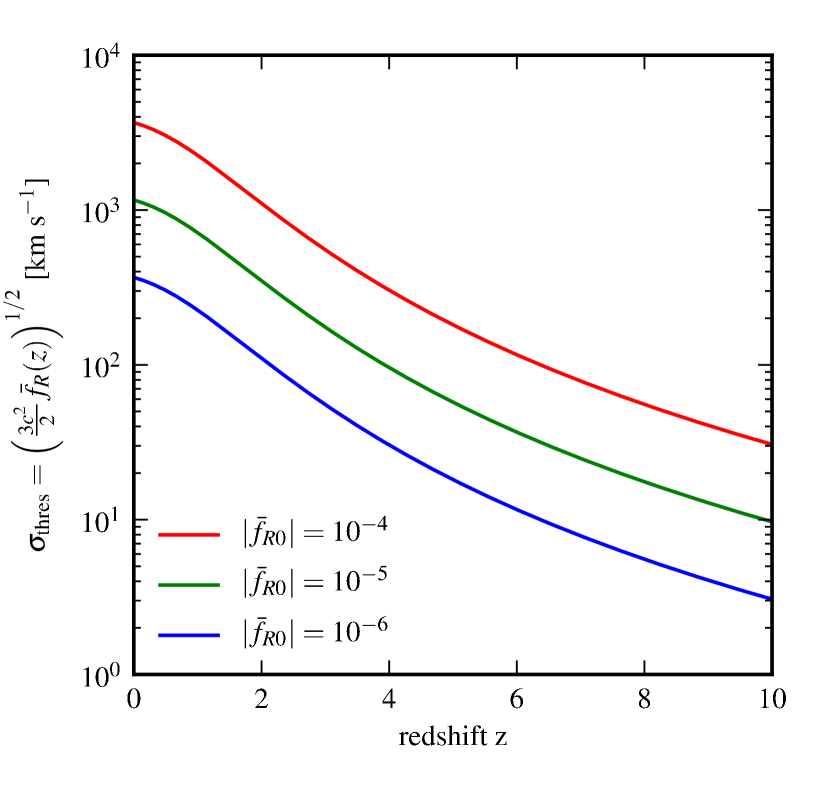
Figure 2: Approximate theoretical threshold value in the three-dimensional halo velocity dispersion for the screening of $f(R)$ effects on gravity due to the chameleon mechanism. In haloes exceeding this threshold, GR gravity is expected to be restored.

4.2 Temperatures of the intracluster and intragroup medium

As the temperature of the intracluster or intragroup medium is closely related to the halo velocity dispersion, we expect to find a similar behaviour in the mass-temperature scaling relation. For the ‘Nonrad’ simulation, this is indeed the case as illustrated in Figure 3, which displays the relation between the group/cluster masses and mass-weighted temperatures, $T_{\rm MW}=\sum T_{\rm particle}m_{\rm particle}/\sum m_{\rm particle}$ within a radius that encloses a mean density of $500$ times the critical density of the Universe. As theoretically expected, the non-radiative $\Lambda$CDM relation follows the slope of the self-similar prediction (Kaiser, 1986), i.e. $T\propto M^{2/3}$, which is indicated by the dashed line in the figure.

In $f(R)$ gravity, the $M$-$T$ relation deviates from the $\Lambda$CDM result. Like the velocity dispersions, the temperatures are boosted by about $30\%-40\%$ with respect to the standard cosmology at masses below approximately $10^{13.8}M_{\odot}$. This increment is again comparable to the enhancement of the gravitational forces. At about $10^{13.8}M_{\odot}$ screening as implied by the chameleon mechanism sets in. This reduces the difference in the $\Lambda$CDM and $f(R)$ relations with increasing mass until the curves coincide for $M_{\rm 500crit}\gtrsim 10^{14.5}M_{\odot}$.

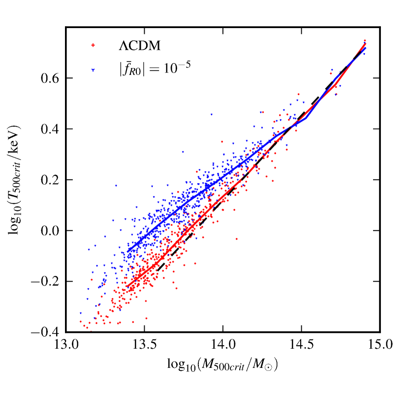
Figure 3: Relation between mass-weighted temperatures and group/cluster masses within $r_{\rm 500crit}$ in the ‘Nonrad’ simulation in a $\Lambda$CDM and a $|\bar{f}_{R0}|=10^{-5}$ cosmology. The solid lines show the median of the binned data, the dashed line indicates the slope of the self-similar scaling relation $T\propto M^{2/3}$.

The masses shown in Figures 1 and 3 were calculated for different spherical overdensity thresholds, i.e. within different radii. To be able to directly compare the enhancement of mass-weighted temperatures and halo velocity dispersions in $f(R)$ gravity, Figure 4 shows the relative difference in the median curves for both quantities. Here, all values were calculated within $r_{\rm 200crit}$. The figure visualizes the theoretically expected effects on both of these quantities. The curves coincide almost perfectly.

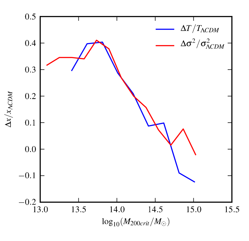
Figure 4: Relative difference between $\Lambda$CDM and $|\bar{f}_{R0}|=10^{-5}$ cosmologies in median velocity dispersion and mass-weighted temperature. All quantities were computed within $r_{\rm 200crit}$. The velocity dispersion was calculated for all friends-of-friends groups while the temperature was computed only for those consisting of at least $2000$ particles.

4.3 Mass bias

4.3.1 Dynamical mass estimates

A standard method for inferring the masses of distant galaxy clusters and groups is to relate the line-of-sight (LOS) velocity dispersion of their member galaxies to their mass by applying the virial theorem. Here, we investigate how these masses are biased in $f(R)$ gravity if modified gravity effects are not specifically corrected for in the analysis, i.e. when the standard relation between velocity dispersion and halo mass is used. To this end, we calculate the LOS velocity dispersion of the subhaloes identified by subfind for massive haloes in our $\Lambda$CDM and $f(R)$ simulations. Based on them, we then estimate the dynamical masses of the haloes with the method described in Bahcall & Tremaine (1981). As the velocity dispersions are enhanced in $f(R)$ gravity one expects the dynamical masses to be higher too. To assess the bias in these mass estimates, we compare the dynamical masses to the true masses, which are simply calculated by summing up the masses of the simulation particles within $r_{\rm 200crit}$.

Figure 5 shows the dynamical mass – true mass relation in $\Lambda$CDM and for $|\bar{f}_{R0}|=10^{-5}$ and $10^{-4}$. For $|\bar{f}_{R0}|=10^{-5}$, we combine results form the ‘DM-small’ and the ‘DM-large’ simulations to cover a larger range in halo mass. The true and dynamical masses of the 40 largest groups of each simulation are indicated by dots in the plot, solid lines show the medians for each cosmology. As expected, the dynamical masses exhibit a similar behaviour as the velocity dispersion. At low masses the dynamical mass estimates in an $f(R)$ cosmology are too high due to the larger dispersion of the subhalo velocities. This clearly demonstrates that in order to obtain accurate masses based on the velocity dispersions, one has to modify the virial theorem instead of using the standard relation which is valid only in GR. At higher masses the chameleon effect sets in and the $f(R)$ dynamical masses are compatible with the GR results. However, even the $\Lambda$CDM curve does not accurately recover the real mass (dashed line) in an intermediate mass region, i.e. around $M_{\rm 200crit}\approx 10^{14.5}M_{\odot}$. This is likely caused by the large scatter implied by the low number of objects.

For $|\bar{f}_{R0}|=10^{-4}$, shown in the figure’s right-hand panel, the behaviour at low masses is the same as in the left hand plot but the dynamical masses are overestimated in the whole mass range displayed in the figure. This is due to the much deeper potential wells that are required for the onset of the chameleon mechanism for larger $|\bar{f}_{R0}|$ values. In the considered mass range they are simply not deep enough for the screening of $f(R)$ effects to become effective. These results are consistent with the behaviour of the velocity dispersions for different $|\bar{f}_{R0}|$ presented in Schmidt (2010).

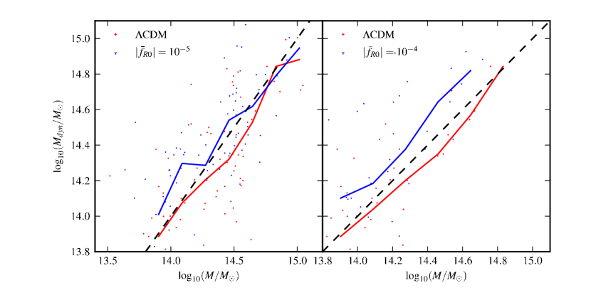
Figure 5: Dynamical vs. real mass for $\Lambda$CDM and $f(R)$ cosmology. The left-hand panel shows the $40$ largest groups of the ‘DM-small’ and ‘DM-large’ simulations, each for $\Lambda$CDM and $|\bar{f}_{R0}|=10^{-5}$ cosmologies. Both simulations use $256^{3}$ particles but differ in box size ($$100\text{\,}\mathrm{M}\mathrm{p}\mathrm{c}$/h$ and $$200\text{\,}\mathrm{M}\mathrm{p}\mathrm{c}$/h$, respectively). The right-hand panel displays the $40$ largest haloes of the ‘DM-high-res’ simulation carried out in $\Lambda$CDM and $|\bar{f}_{R0}|=10^{-4}$ cosmologies. All results are based on collisionless simulations. The dynamical masses are computed with the method described in Bahcall & Tremaine (1981) using the velocity dispersion of the subhaloes identified by subfind to represent the velocity dispersion of cluster galaxies. Solid lines indicate the median of the binned data, dashed lines the 1:1 relation.

The increment in dynamical masses is caused by the higher subhalo velocity-dispersion in $f(R)$ gravity. In contrast, there is only a small difference in subhalo abundance between modified gravity and GR in our simulations. This is illustrated in Figure 6.

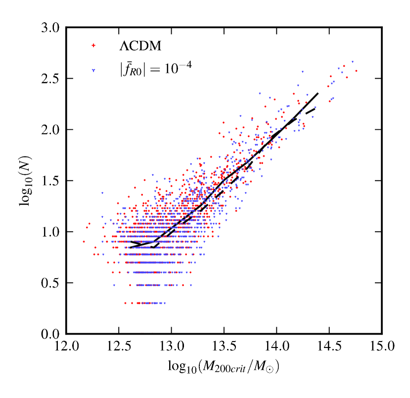
Figure 6: Number $N$ of resolved subhaloes as a function of the mass of the parent halo. Only objects for which the main halo is resolved by at least 2000 simulation particles in the ‘DM-high-res’ simulations are included. The lines show the medians of the binned data for $\Lambda$CDM (solid line) and $f(R)$ (dashed line).

4.3.2 Hydrostatic masses

Our hydrodynamical simulations offer the opportunity to investigate cluster mass estimates that are based on the properties of the ICM, a method which is used as a standard technique to interpret X-ray observations of galaxy clusters. These so called hydrostatic masses are compared to the true mass in Figure 7. The medians are indicated by solid lines. The dashed line shows the 1:1 relation. Hydrostatic masses are estimated from the pressure gradient at $r_{\rm 500crit}$.

To obtain results which are as realistic as possible for the given simulation, both thermal and non-thermal pressure contributions were considered. The thermal pressure is calculated from the temperatures of the gas particles while the non-thermal part is computed from the velocities of the simulation particles relative to their host halo. The latter corresponds to bulk motions in the ICM. Effectively, the pressure is, thus, computed based on the sum of the thermal and the kinetic energy (in the object’s rest frame) of the ICM.

The non-thermal pressure defined in this way can, however, be easily overestimated in merging clusters. Furthermore, in those objects the hydrostatic equilibrium assumption is likely violated. To prevent our results from being strongly affected by mergers, we introduce a criterion for the selection of clusters. Only objects whose average kinetic particle energy around $r_{\rm 500crit}$ does not exceed $0.5$ times the thermal energy of the particles are considered in the analysis. Additionally, criteria for identifying relaxed systems, based on considering the centre-of-mass displacement and the mass in substructures, were applied. These criteria are similar to those used in Neto et al. (2007). If the distance from the centre-of-mass to the minimum of the gravitational potential is larger than $0.105\times r_{\rm 200crit}$, the object is considered as not relaxed and excluded from the analysis. The same is the case if the mass of the substructures found by subfind exceeds $10\%$ of the total cluster mass. As the plot shows, these criteria ensure that hydrostatic and true mass are in good agreement in the $\Lambda$CDM model. It was also checked that the selection criteria do not bias the results in $f(R)$ gravity. In particular, we found that there is no significant difference in the fraction of relaxed objects at fixed halo mass in $f(R)$ gravity compared to $\Lambda$CDM. The ratio of thermal to non-thermal pressure remains also unchanged.

For the $f(R)$ cosmology, the hydrostatic masses were computed in the same way as for $\Lambda$CDM. In particular, modified gravity effects were not explicitly accounted for in the mass estimates. These estimates, thus, correspond to hydrostatic masses computed from observations assuming that the observer is unaware of the presence of modifications of gravity. As expected, this results in an overestimate of the true mass due to the modified relation between the mass distribution and the gravitational potential. As a cautionary remark, we would like to add that this mass bias should not be confused with hydrostatic mass biases that may arise in $\Lambda$CDM due to violations of the hydrostatic equilibrium condition or due to unaccounted non-thermal pressure components.

To compare the simulations to recent observational data, the results found by the Planck Collaboration (2013) were added to the plot (green symbols). Like for the simulations, the hydrostatic masses $M^{\rm hydro}_{500}$ are shown on the figure’s vertical axis, while the horizontal axis displays weak lensing masses $M^{\rm WL}_{500}$. Except for observational errors in the weak lensing analysis, the latter can be considered to represent the true mass as lensing deflection angles and mass estimates are not altered by $f(R)$-gravity effects in models with $|\bar{f}_{R0}|\ll 1$ (see Appendix A and Zhao et al., 2011b). The best fit region from that work, $M^{\rm WL}_{500}=(0.78\pm 0.08)M^{\rm hydro}_{500}$, is shaded in green.

Like in our $f(R)$ simulations, the Planck Collaboration (2013) found hydrostatic masses which are larger than the corresponding weak lensing masses. If this result is, indeed, substantiated by future studies and not caused by some observational bias, modified gravity could provide a theoretical explanation for it. One should keep in mind, however, that there are observational uncertainties that might also cause such a bias (some of them are discussed in Planck Collaboration et al. 2013, as well as in Applegate et al. 2012). Furthermore, there are also authors that find that hydrostatic masses are smaller than weak lensing masses (Mahdavi et al., 2013). Finally, we have to acknowledge that $|\bar{f}_{R0}|=10^{-5}$ might already be in tension with Solar system constraints (Hu & Sawicki, 2007). However, given that the onset of screening is not visible in Fig. 7 even for the most massive simulated clusters (see discussion below), it is quite possible that higher hydrostatic cluster masses also appear for somewhat lower $|\bar{f}_{R0}|$.

Comparing the mass difference in Figure 7 to the previous plots, one might be surprised why the effects of a chameleon screening of $f(R)$ gravity for objects with masses above $10^{14}M_{\odot}$ are not clearly visible, as this was the case for the previously analysed quantities and $|\bar{f}_{R0}|=10^{-5}$. The reason is most likely that the quantities in the other plots are calculated by averaging over the whole volume within the considered radius, while the hydrostatic masses are computed using the pressure and potential gradients at a relatively large specific radius, i.e. at $r_{\rm 500crit}$. It is, hence, more sensitive to the cluster outskirts, where the potential is not as deep as in the central region. This shifts the transition of the screened regime to larger cluster masses. As a consequence, the lack of more massive clusters in our simulations prevents us from seeing this transition in Fig. 7.

The increased dynamical and hydrostatic masses in $f(R)$ gravity are consistent with the theoretical expectations. Since gravity is enhanced by a factor of up to $4/3$ with respect to GR one expects an enhancement of mass estimates of the same order (Schmidt et al. 2009). Figures 5 and 7, indeed, show that an increment of this order is present in our results.

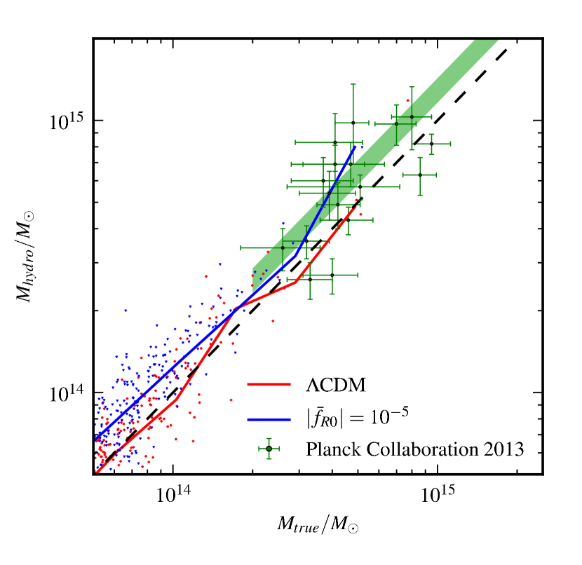
Figure 7: Relation between hydrostatic mass estimates and the true mass for relaxed (see text) clusters in the $\Lambda$CDM (red) and $|\bar{f}_{R0}|=10^{-5}$ (blue) simulations, respectively. Solid lines show the median of the binned data, the dashed line indicates the 1:1 relation. The green symbols with error bars are the data points of the Planck Collaboration (2013) (hydrostatic and weak lensing masses) and the green shaded region represent their best fit region. All values are measured within $r_{\rm 500crit}$. For the $f(R)$ model, mass estimates were computed assuming an observer is unaware of modified gravity effects.

4.4 Scaling relations

4.4.1 The $L$-$T$ scaling relation

Our ‘Nonrad’ simulations follow the evolution of the density and temperature distributions of the ICM. This allows us to investigate the X-ray properties of our simulated clusters. In particular, we calculate emission-weighted temperatures and X-ray luminosities for all clusters and groups found by subfind. To calculate the luminosity, metal line emission was neglected as the exact shape of the cooling function is unlikely to have a qualitative impact on the comparison between different cosmological models. Furthermore, the simulations do not follow the metal enrichment of the ICM, so that ad hoc assumptions about the metallicity would be necessary to include line emission. Finally, to be able to directly compare our simulated scaling relation to observations, it would be necessary to account for additional baryonic physics that is important in this context, like star formation and feedback from active galactic nuclei (see e.g. Puchwein et al., 2008).

We, hence, stick to the simple assumption of free–free bremsstrahlung and compute the luminosities according to $L\propto\sum\rho m\sqrt{T}$, where $\rho$ is the gas density, $T$ the gas temperature and $m$ the gas particle mass. The sum extends over all gas particles within $r_{\rm 500crit}$. The emission-weighted temperatures are estimated by weighting the temperatures of the gas particles within the same radius with their estimated X-ray luminosity.

Figure 8 shows the relation between X-ray luminosity and temperature for all groups and clusters which are resolved by at least 200 particles. Results are shown both for a $\Lambda$CDM and a $|\bar{f}_{R0}|=10^{-5}$ cosmology. The luminosities at fixed temperature are lower in $f(R)$ gravity compared to $\Lambda$CDM. This is not unexpected: as shown in Figure 3, the temperature of the ICM at a given halo mass is larger in $f(R)$ gravity. Or in other words, the mass of an object at given temperature will be lower in $f(R)$. Given that the luminosity is roughly proportional to $\sim M\sqrt{T}$, a lower mass $M$ translates to a lower X-ray luminosity. Also note that the slope of the cooling rate as a function of temperature would be even lower in the relevant range if metal cooling were accounted for. Including metal line cooling would, thus, not qualitatively change our results. As expected, the difference between the models decreases at high temperatures where the chameleon mechanism becomes effective.

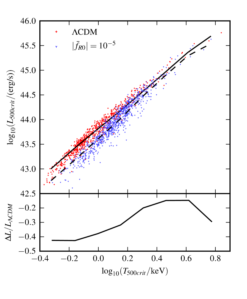
Figure 8: Upper panel: X-ray luminosities of clusters and groups as a function of their emission-weighted temperature. Results are shown for a $|\bar{f}_{R0}|=10^{-5}$ (blue, dashed line) and a $\Lambda$CDM (red, solid line) cosmology. The values are computed within $r_{\rm 500crit}$ for all objects resolved by at least 2000 simulation particles. The lines show the medians of the binned data. Lower panel: Relative difference of the medians shown in the upper panel.

4.4.2 The $Y_{\rm SZ}$-$M$ scaling relation

Another observational probe of the intracluster and intragroup medium is the spectral distortion of the cosmic microwave background that is caused by foreground galaxy clusters and groups. This distortion, known as the thermal SZ effect, can be described by the Compton-$y$ parameter, which is a scaled projection of the gas pressure in the intervening cluster or group. Integrating the Compton-$y$ parameter over the projected extent of the objects on the sky yields $Y_{\rm SZ}$, which correlates well with halo mass.

The relation between $Y_{\rm SZ}$ and mass is shown in Figure 9. It is computed using the temperatures and masses of the gas particles in the ‘Nonrad’ simulation outputs of both the $\Lambda$CDM and the $|\bar{f}_{R0}|=10^{-5}$ runs. The integrated Compton parameter is plotted against true and hydrostatic masses, where the latter have been computed in the same way as for Figure 7. Comparing the $Y_{\rm SZ}$-true mass relations, we find larger $Y_{\rm SZ}$ values in $f(R)$ than in $\Lambda$CDM. This is expected since $Y_{\rm SZ}$ depends on the electron temperatures which are larger in $f(R)$ gravity. Like for many of the previously analysed quantities, the difference between the models decreases at about ${10^{14}}{M_{\odot}}$ due to the chameleon mechanism becoming effective there.

As expected from Fig. 7, the $Y_{\rm SZ}$-hydrostatic mass relation, which could be probed by a comparison of X-ray and SZ data, is basically identical to the $Y_{\rm SZ}$-true mass relation in $\Lambda$CDM. In contrast, the $Y_{\rm SZ}$-mass relation strongly depends on the mass measure in $f(R)$ gravity. Larger hydrostatic masses in the $f(R)$ model shift the curve to the right. Interestingly, the $Y_{\rm SZ}$-hydrostatic mass relation is rather similar in $\Lambda$CDM and $f(R)$. Larger hydrostatic masses almost compensate the stronger SZ signal. This results in a shift mostly along the relation, rather than perpendicular to it. In observed scaling relations, it will therefore be easier to see effects of $f(R)$ gravity in the $Y_{\rm SZ}$-lensing mass relation.

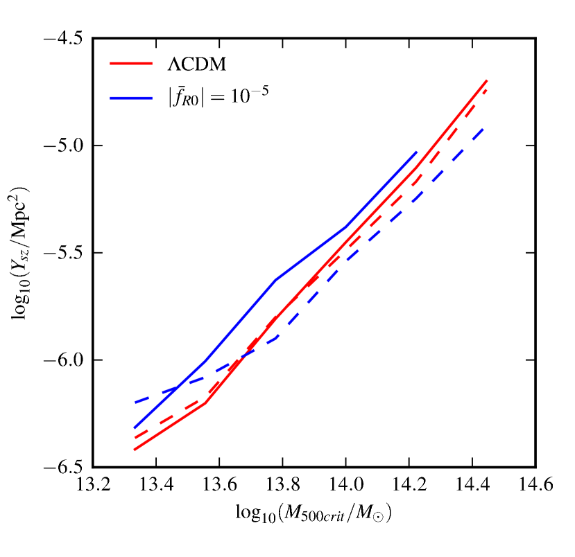
Figure 9: Integrated thermal SZ signal $Y_{\rm SZ}$ as a function of true (solid lines) and hydrostatic (dashed lines) mass for the $\Lambda$CDM (red) and the $|\bar{f}_{R0}|=10^{-5}$ (blue) cosmologies. The lines show the median values for all groups which fit the criteria for relaxed systems (see Sec. 4.3.2). Hydrostatic masses were estimated in the same way as for Figure 7.

5 Summary and conclusions

We have performed the first analysis of galaxy clusters and groups in cosmological hydrodynamical simulations of $f(R)$ gravity models, using the Hu & Sawicki (2007) parametrization. In addition, we have studied collisionless runs of the same model, as well as reference $\Lambda$CDM simulations. The hydrodynamical simulations allowed us to explore the effects of modified gravity on the ICM and its observable properties, as well as on hydrostatic mass estimates and X-ray and SZ scaling relations. The dynamics of cluster galaxies, as traced by self-bound subhaloes, were investigated both in hydrodynamical and collisionless runs. The effects of modified gravity on dynamical mass estimates were determined. Our main findings are the following.

• The dark matter velocity dispersions of low-mass haloes are boosted by roughly a factor $\sqrt{4/3}$ in $f(R)$ gravity compared to $\Lambda$CDM. This is consistent both with previous works (Schmidt 2010) and theoretical expectations, given that gravitational forces are increased by a factor of $4/3$ in these objects.

• The maximum halo mass for which this enhanced velocity dispersion is observed depends of the value $|\bar{f}_{R0}|$, as it controls in which objects the chameleon mechanism is effective. For $|\bar{f}_{R0}|=10^{-6}$ modified gravity effects are screened in almost the whole mass range we have explored, so that no changes in the velocity dispersions compared to $\Lambda$CDM are observed. For $|\bar{f}_{R0}|=10^{-5}$, velocity dispersions are increased below $\sim 10^{14.5}M_{\odot}$ and show little difference above this value. For $|\bar{f}_{R0}|=10^{-4}$, there is no screening even in massive clusters, so that velocity dispersions are boosted in all haloes in this case. We show that this trend is consistent with theoretical expectations.

• The mass-temperature scaling relation is affected by $f(R)$ gravity. More precisely, in unscreened, i.e. less massive haloes the temperature at fixed mass increases with respect to $\Lambda$CDM. In particular, we find that the gas temperatures and the variance of the dark matter velocities are boosted by the same halo mass-dependent factor.

• $f(R)$ gravity not only increases the velocity dispersion of dark matter particles, but also the dispersion of subhalo velocities. This translates into a bias in dynamical mass estimates. More precisely, halo masses estimated based on subhalo velocities overpredict the true mass in unscreened haloes unless modified gravity effects are explicitly accounted for in the analysis. In massive haloes in which the chameleon mechanism is effective, the dynamical masses are in good agreement with the true masses. The abundance of subhaloes is only very mildly affected by $f(R)$ gravity.

• Hydrostatic masses are also increased in $f(R)$ gravity compared to $\Lambda$CDM if modified gravity effects are not explicitly accounted for in the mass estimate. In contrast to the previously analysed quantities, we do not see a transition from the unscreened to the screened regime in the hydrostatic mass-true mass relation in our non-radiative hydrodynamical simulation. This has most likely the following reason: hydrostatic masses were computed from the pressure gradient at a specific, relatively large radius, namely $r_{\rm 500crit}$. There the gravitational potential is not as deep as in the central cluster or group region. Thus, at these large radii the transition between the unscreened and the screened regime is shifted towards more massive objects which are not present in the analysed simulations.

• While hydrostatic masses are biased in $f(R)$ gravity, lensing mass estimates are not affected. This results in an offset in the X-ray mass-lensing mass relation of roughly the same magnitude as recently found by the Planck Collaboration (2013). If their finding is substantiated by future studies, modified gravity could provide an explanation for this offset.

• We find a lower normalization of the X-ray luminosity-temperature scaling relation in $f(R)$ gravity. The increment in X-ray luminosities in $f(R)$ gravity is overcompensated by the boosted temperatures. This results in a lower normalization of the $L-T$ relation for objects in which modified gravity is not efficiently screened.

• The SZ signal of our simulated clusters and groups is affected by $f(R)$ gravity as well. The effect on the $Y_{\rm SZ}-M$ relation depends, however, significantly on the mass measure which is used. When plotted against hydrostatic masses, the relation in $f(R)$ gravity is only shifted along the GR-curve since both quantities are enhanced. The $f(R)$ effects on the SZ signal are much more clearly visible if $Y_{\rm SZ}$ is displayed as a function of true or lensing mass.

Overall, our analysis demonstrates that $f(R)$ gravity significantly affects the velocity dispersions, virial temperatures and scaling relations of unscreened haloes. Furthermore, an observer who is unaware of modifications of gravity would obtain biased mass estimates both from a dynamical analysis, as well as based on the assumption of hydrostatic equilibrium in a Newtonian potential.

In the future, it will be interesting to include further baryonic physics in cosmological hydrodynamical simulations of modified gravity, as well as to push to higher resolution. This will allow investigating modified gravity effects on galaxies and galaxy populations self-consistently, thereby complementing work based on semi-analytical galaxy formation models (see Fontanot et al., 2013).

Appendix A The modified Poisson equation and lensing masses in ${f}(R)$ gravity

The aim of this appendix is to derive the modified Poisson equation for $f(R)$ gravity (Eq. 4) and the equation for the scalar degree of freedom (Eq. 3), as well as to show that the relations between mass density and lensing deflection angles are identical in $f(R)$ gravity and GR. This ensures that lensing masses are not biased by $f(R)$ modifications of gravity.

Adopting the Newtonian gauge and assuming for simplicity a spatially flat background, the line element can be written as

$${\rm d}s^{2}=a(\eta)^{2}\left[-(1+2\Phi){\rm d}\eta^{2}+(1-2\Psi){\rm d}\mathbf{x}^{2}\right],$$ (13)

where $\eta$ denotes conformal time and is related to cosmic time $t$ by $a(\eta){\rm d}\eta\equiv{\rm d}t$. In this metric gravitational lensing is governed by $\Phi_{L}=(\Phi+\Psi)/2$ (Bartelmann 2010; Zhao et al. 2011b). To simplify the calculations, we define $F=f_{R}+1$ and rewrite Eq. (2) as

$$FR_{\mu\nu}-\frac{1}{2}fg_{\mu\nu}-\frac{1}{2}Rg_{\mu\nu}-\nabla_{\mu}\nabla_{\nu}F+g_{\mu\nu}\Box F=8\pi GT_{\mu\nu},$$ (14)

where the d’Alembert operator is defined by $\Box=g^{\mu\nu}\nabla_{\mu}\nabla_{\nu}$. Taking the trace of Eq. (14) leads to

$$FR-2f-2R+3\Box F=8\pi GT.$$ (15)

A.1 The equation for $f_{R}$

As $|f_{R}|\ll 1$ in all models we consider, we can approximate $F\approx 1$ in the first term of Eq. (15). Subtracting the background equation from the result and neglecting a $\delta f$ term, as $|\delta f|\approx|f_{R}\delta R|\ll|\delta R|$, yields

$$\Box f_{R}=\frac{1}{3}\left(\delta R-8\pi G\delta\rho\right),$$ (16)

where the energy-momentum tensor was assumed to be that of a pressure-less fluid, so that $\delta T=-\delta\rho$, and $\delta\rho$ is the perturbation in physical density. In the quasi-static limit, i.e. neglecting all time derivatives and assuming instantaneous propagation of gravity (see Noller et al., 2014, for a discussion of the validity of this assumption), this equation turns into

$$\frac{1}{a^{2}}\nabla^{2}f_{R}=\nabla^{2}_{\rm phys}f_{R}=\frac{1}{3}\left(\delta R-8\pi G\delta\rho\right),$$ (17)

where $\nabla^{2}$ and $\nabla^{2}_{\rm phys}$ denote the Laplace operators with respect to comoving and physical coordinates, respectively. The second equality is identical to Eq. (3), except that we have omitted the subscript in $\nabla^{2}_{\rm phys}$ in the latter equation for the sake of brevity.

A.2 The modified Poisson equation for the gravitational potential

Taking the $00$-component of Eq. (14) and plugging it into the metric Eq. (13) yields

$$FR_{00}+\frac{1}{2}(f+R)a^{2}(1+2\Phi)-\frac{1+2\Phi}{1-2\Psi}\nabla^{2}F=8\pi G\rho\,a^{2}.$$ (18)

The second time derivative of $F$, corresponding to the fourth term of Eq. (14), has here been canceled by the time component of the D’Alembert operator. The energy-momentum tensor was assumed to have the pressure-less perfect fluid form, i.e. $T_{00}=\rho\,a^{2}$.

In the following we adopt the weak field limit, i.e. we assume $|\Phi|\ll 1$ and $|\Psi|\ll 1$, and consider models with $|f_{R}|\ll 1$, so that we can approximate $F\approx 1$ in the first term. After subtracting the background equation, we find

$$\delta R_{00}+\frac{1}{2}\delta R\,a^{2}-\nabla^{2}f_{R}=8\pi G\delta\rho\,a^{2},$$ (19)

where $|\delta f|\approx|f_{R}\delta R|\ll|\delta R|$ has been used. Plugging in (17), one obtains

$$\delta R_{00}=\frac{16\pi G}{3}\delta\rho\,a^{2}-\frac{1}{6}\delta R\,a^{2}.$$ (20)

A similar calculation for the space-space components of (14) leads to

$$\delta R_{ii}-\frac{1}{2}\delta R\,a^{2}-\nabla_{i}\nabla_{i}\delta f_{R}+\nabla^{2}\delta f_{R}=0,$$ (21)

where we have again assumed $|\Phi|\ll 1$, $|\Psi|\ll 1$ and have adopted the quasi-static approximation. Summing over the spatial components, one obtains

$$\sum_{i=1}^{3}\delta R_{ii}-\frac{3}{2}\delta R\,a^{2}+2\nabla^{2}\delta f_{R}=0,$$ (22)

Using (17) and sorting terms yields

$$\sum_{i=1}^{3}\delta R_{ii}=\frac{16\pi G}{3}\delta\rho\,a^{2}+\frac{5}{6}\delta R\,a^{2}.$$ (23)

To obtain the Ricci tensor for the considered metric (13), the Christoffel symbols

$$\Gamma^{\kappa}_{\mu\nu}=\frac{1}{2}g^{\kappa\alpha}(g_{\alpha\nu,\mu}+g_{\mu\alpha,\nu}-g_{\mu\nu,\alpha})$$ (24)

must be calculated. Denoting derivatives with respect to conformal time and spatial comoving coordinates as $x^{\prime}\equiv\partial_{\eta}x$ and $x_{,j}\equiv\partial_{j}x$, the components can be written as

$$\Gamma^{0}_{00} =\frac{a^{\prime}}{a}+\Phi^{\prime},\quad \Gamma^{i}_{00} =\Phi_{,i}\;\;,$$

$$\Gamma^{0}_{0i} =\Phi_{,i}\;\;,\quad \Gamma^{i}_{0j} =\left(\frac{a^{\prime}}{a}-\Psi^{\prime}\right)\delta^{i}_{j},$$

$$\Gamma^{0}_{ij} =\left(\frac{a^{\prime}}{a}\left[1-2(\Phi+\Psi)\right]-\Psi^{\prime}\right)\delta_{ij},$$

$$\Gamma^{i}_{jk} =\Psi_{,i}\delta_{jk}-\Psi_{,j}\delta^{i}_{k}-\Psi_{,k}\delta^{i}_{j}.$$ (25)

The Ricci tensor can be computed from the connection forms as

$$R_{\mu\nu}=\Gamma^{\kappa}_{\mu\nu,\kappa}-\Gamma^{\kappa}_{\kappa\mu,\nu}+\Gamma^{\kappa}_{\kappa\gamma}\Gamma^{\gamma}_{\nu\mu}-\Gamma^{\kappa}_{\nu\gamma}\Gamma^{\gamma}_{\kappa\mu}.$$ (26)

Neglecting second and higher order terms in $\Phi$ and $\Psi$ the diagonal elements turn out to be

$$R_{00} = -3\mathcal{H}^{\prime}+3\Psi^{\prime\prime}+\nabla^{2}\Phi+3\mathcal{H}(\Phi^{\prime}+\Psi^{\prime}),$$ (27)

$$R_{ii} = (\mathcal{H}^{\prime}+2\mathcal{H}^{2})$$

$$+ \left[-\Psi^{\prime\prime}+\nabla^{2}\Psi-\mathcal{H}(\Phi^{\prime}+5\Psi^{\prime})-(2\mathcal{H}^{\prime}+4\mathcal{H}^{2})(\Phi+\Psi)\right]$$

$$+ \nabla_{i}\nabla_{i}(\Psi-\Phi),$$ (28)

in the coordinates defined by Eq. (13). Here, $\mathcal{H}=a^{\prime}/a$ is the conformal Hubble function. In the quasi-static regime and on scales much smaller than the Hubble radius, we can neglect all time derivatives of $\Phi$ and $\Psi$, as well as factors of $\mathcal{H}$ and its derivatives. This yields

$$\delta R_{00} = \,\,\,\nabla^{2}\Phi,$$ (29)

$$\sum_{i=1}^{3}\delta R_{ii} = \,\,\,3\,\nabla^{2}\Psi+\nabla^{2}(\Psi-\Phi)=4\,\nabla^{2}\Psi-\nabla^{2}\Phi.$$ (30)

Combining equations (20) and (29) results in the modified Poisson equation (Eq. 4) for the gravitational potential

$$\frac{1}{a^{2}}\nabla^{2}\Phi=\nabla^{2}_{\rm phys}\Phi=\frac{16\pi G}{3}\delta\rho-\frac{1}{6}\delta R.$$ (31)

A.3 Gravitational lensing in $f(R)$ gravity

Using this result together with (23) and (30) leads to a similar relation for $\Psi$

$$\frac{1}{a^{2}}\nabla^{2}\Psi=\nabla^{2}_{\rm phys}\Psi=\frac{8\pi G}{3}\delta\rho+\frac{1}{6}\delta R.$$ (32)

Thus the potential $\Phi_{L}=(\Psi+\Phi)/2$, which governs gravitational light deflection, satisfies

$$\nabla^{2}_{\rm phys}\Phi_{L}=\frac{\nabla^{2}_{\rm phys}\Phi+\nabla^{2}_{\rm phys}\Psi}{2}=4\pi G\delta\rho=\nabla^{2}_{\rm phys}\phi_{\rm N},$$ (33)

i.e. it satisfies the same standard Poisson equation as the Newtonian gravitational potential $\phi_{\rm N}$, and is hence unchanged despite the $f(R)$ effects on $\Phi$ and $\Psi$. As a consequence, the gravitational lensing deflection angle

$$\boldsymbol{\alpha}=\frac{2}{c^{2}}\int\boldsymbol{\nabla}_{\perp}\left(\frac{\Phi+\Psi}{2}\right)\,{\rm d}l=\frac{2}{c^{2}}\int\boldsymbol{\nabla}_{\perp}\phi_{\rm N}\,{\rm d}l,$$ (34)

is the same as in GR. Here $\boldsymbol{\nabla}_{\perp}$ is the component of the gradient with respect to physical coordinates which is perpendicular to the line of sight. The line element ${\rm d}l$ corresponds to proper distance. Weak lensing mass estimates are, thus, not affected by $f(R)$ gravity in models with $|\bar{f}_{R0}|\ll 1$.

References

- Applegate et al. (2012) Applegate D. E. et al., 2012, ArXiv e-prints: 1208.0605
- Bahcall & Tremaine (1981) Bahcall J. N., Tremaine S., 1981, ApJ, 244, 805
- Bartelmann (2010) Bartelmann M., 2010, Classical and Quantum Gravity, 27, 233001
- Buchdahl (1970) Buchdahl H. A., 1970, MNRAS, 150, 1
- Cabré et al. (2012) Cabré A., Vikram V., Zhao G.-B., Jain B., Koyama K., 2012, JCAP, 7, 34
- Cai et al. (2013) Cai Y.-C., Li B., Cole S., Frenk C. S., Neyrinck M., 2013, ArXiv e-prints: 1310.6986
- Deffayet et al. (2002) Deffayet C., Dvali G., Gabadadze G., Vainshtein A., 2002, Phys. Rev. D, 65, 044026
- Ferraro et al. (2011) Ferraro S., Schmidt F., Hu W., 2011, Phys. Rev. D, 83, 063503
- Fontanot et al. (2013) Fontanot F., Puchwein E., Springel V., Bianchi D., 2013, MNRAS, 436, 2672
- Gasperini et al. (2002) Gasperini M., Piazza F., Veneziano G., 2002, Phys. Rev. D, 65, 023508
- Hinterbichler & Khoury (2010) Hinterbichler K., Khoury J., 2010, Physical Review Letters, 104, 231301
- Hu & Sawicki (2007) Hu W., Sawicki I., 2007, Phys. Rev. D, 76, 064004
- Jennings et al. (2012) Jennings E., Baugh C. M., Li B., Zhao G.-B., Koyama K., 2012, MNRAS, 425, 2128
- Kaiser (1986) Kaiser N., 1986, MNRAS, 222, 323
- Khoury & Weltman (2004) Khoury J., Weltman A., 2004, Phys. Rev. D, 69, 044026
- Lam et al. (2012) Lam T. Y., Nishimichi T., Schmidt F., Takada M., 2012, Physical Review Letters, 109, 051301
- Li et al. (2013) Li B., Hellwing W. A., Koyama K., Zhao G.-B., Jennings E., Baugh C. M., 2013, MNRAS, 428, 743
- Li et al. (2012) Li B., Zhao G.-B., Teyssier R., Koyama K., 2012, JCAP, 1, 51
- Li & Hu (2011) Li Y., Hu W., 2011, Phys. Rev. D, 84, 084033
- Llinares et al. (2013) Llinares C., Mota D. F., Winther H. A., 2013, arXiv: 1307.6748
- Lombriser et al. (2012a) Lombriser L., Koyama K., Zhao G.-B., Li B., 2012a, Phys. Rev. D, 85, 124054
- Lombriser et al. (2012b) Lombriser L., Schmidt F., Baldauf T., Mandelbaum R., Seljak U., Smith R. E., 2012b, Phys. Rev. D, 85, 102001
- Mahdavi et al. (2013) Mahdavi A., Hoekstra H., Babul A., Bildfell C., Jeltema T., Henry J. P., 2013, ApJ, 767, 116
- Neto et al. (2007) Neto A. F. et al., 2007, MNRAS, 381, 1450
- Noller et al. (2014) Noller J., von Braun-Bates F., Ferreira P. G., 2014, Phys. Rev. D, 89, 023521
- Oyaizu (2008) Oyaizu H., 2008, Phys. Rev. D, 78, 123523
- Planck Collaboration et al. (2013) Planck Collaboration et al., 2013, A&A, 550, A129
- Puchwein et al. (2013) Puchwein E., Baldi M., Springel V., 2013, MNRAS, 436, 348
- Puchwein et al. (2008) Puchwein E., Sijacki D., Springel V., 2008, ApJ, 687, L53
- Schmidt (2010) Schmidt F., 2010, Phys. Rev. D, 81, 103002
- Schmidt et al. (2009) Schmidt F., Lima M., Oyaizu H., Hu W., 2009, Phys. Rev. D, 79, 083518
- Springel (2005) Springel V., 2005, MNRAS, 364, 1105
- Springel & Hernquist (2002) Springel V., Hernquist L., 2002, MNRAS, 333, 649
- Springel et al. (2001) Springel V., White S. D. M., Tormen G., Kauffmann G., 2001, MNRAS, 328, 726
- Vainshtein (1972) Vainshtein A., 1972, Physics Letters B, 39, 393
- Zhao et al. (2011a) Zhao G.-B., Li B., Koyama K., 2011a, Phys. Rev. D, 83, 044007
- Zhao et al. (2011b) Zhao G.-B., Li B., Koyama K., 2011b, Physical Review Letters, 107, 071303