A Merger Shock in Abell 2034.

Matt S. Owers¹¹affiliation: Australian Astronomical Observatory, PO Box 915, North Ryde, NSW 1670, Australia ⁵⁵affiliation: Australian Research Council Super Science Fellow; Email: matthew.owers@aao.gov.au , Paul E.J. Nulsen²²affiliation: Harvard Smithsonian Center for Astrophysics, 60 Garden Street, Cambridge, MA 02138, USA , Warrick J. Couch¹¹affiliation: Australian Astronomical Observatory, PO Box 915, North Ryde, NSW 1670, Australia ³³affiliation: Center for Astrophysics and Supercomputing, Swinburne University of Technology, Hawthorn, VIC 3122, Australia , Cheng-Jiun Ma²²affiliation: Harvard Smithsonian Center for Astrophysics, 60 Garden Street, Cambridge, MA 02138, USA ⁴⁴affiliation: Department of Physics & Astronomy, University of Waterloo, 200 University Ave. W., Waterloo, Ontario, N2L 3G1, Canada , Laurence P. David²²affiliation: Harvard Smithsonian Center for Astrophysics, 60 Garden Street, Cambridge, MA 02138, USA , William R. Forman²²affiliation: Harvard Smithsonian Center for Astrophysics, 60 Garden Street, Cambridge, MA 02138, USA , Andrew M. Hopkins¹¹affiliation: Australian Astronomical Observatory, PO Box 915, North Ryde, NSW 1670, Australia , Christine Jones²²affiliation: Harvard Smithsonian Center for Astrophysics, 60 Garden Street, Cambridge, MA 02138, USA , Reinout J. van Weeren²²affiliation: Harvard Smithsonian Center for Astrophysics, 60 Garden Street, Cambridge, MA 02138, USA

Abstract

We present a 250 ks Chandra observation of the cluster merger A2034 with the aim of understanding the nature of a sharp edge previously characterized as a cold front. The new data reveal that the edge is coherent over a larger opening angle and is significantly more bow-shock-shaped than previously thought. Within $\sim 27\arcdeg$ about the axis of symmetry of the edge the density, temperature and pressure drop abruptly by factors of $1.83^{+0.09}_{-0.08}$ , $1.85^{+0.41}_{-0.41}$ and $3.4^{+0.8}_{-0.7}$ , respectively. This is inconsistent with the pressure equilibrium expected of a cold front and we conclude that the edge is a shock front. We measure a Mach number $M=1.59^{+0.06}_{-0.07}$ and corresponding shock velocity $v_{\rm shock}\simeq 2057$ $\,\rm{km\,s^{-1}}$ . Using spectra collected at the MMT with the Hectospec multi-object spectrograph we identify 328 spectroscopically confirmed cluster members. Significantly, we find a local peak in the projected galaxy density associated with a bright cluster galaxy which is located just ahead of the nose of the shock. The data are consistent with a merger viewed within $\sim 23\arcdeg$ of the plane of the sky. The merging subclusters are now moving apart along a north-south axis approximately $0.3\,$ Gyr after a small impact parameter core passage. The gas core of the secondary subcluster, which was driving the shock, appears to have been disrupted by the merger. Without a driving “piston” we speculate that the shock is dying. Finally, we propose that the diffuse radio emission near the shock is due to the revival of pre-existing radio plasma which has been overrun by the shock.

Subject headings:

galaxies: clusters: individual (Abell 2034) — X-rays: galaxies: clusters

1. Introduction

Cluster mergers are natural outcomes of the hierarchical nature of large scale structure formation. Major mergers involving clusters of a similar mass are rare, although the impact on the cluster constituents can be significant given the extreme kinetic energies of up to $10^{64}\,$ erg (markevitch1999). Approximately $10\%$ of this energy is dissipated in the collisional intracluster medium (ICM) through shocks, turbulence and compression which produce spectacular observable effects at X-ray wavelengths (markevitch2007; sarazin2008). Observations of cluster mergers have proven valuable in constraining the nature of dark matter (e.g., in the Bullet cluster; clowe2006; randall2008b), the cosmic ray content of clusters (feretti2012), the intracluster magnetic field strength (vikhlinin2001a), and for understanding the physics of the ICM (ettori2000; vikhlinin2001b; russell2012; roediger2013). These studies show that deep multiwavelength observations of cluster mergers are critical if we are to understand the impact of large scale structure formation on the cluster constituents.

Early X-ray observations of cluster mergers using the ROSAT and ASCA satellites revealed a hot, apparently shock-heated ICM in regions affected by merger activity (henriksen1996; donelly1998; markevitch1999). However, the spatial resolution was not sufficient to see the surface brightness edge expected due to the compression of gas at the shock front. The launch of the Chandra X-ray observatory with its sub-arcsecond resolution and excellent sensitivity was expected to reveal many shock edges in merging clusters. In fact, while Chandra has uncovered a number of merger-related edges, the vast majority are cold fronts (markevitch2000; vikhlinin2002; owers2009c) and only a handful of shock fronts have been directly observed as sharp edges in Chandra images (in the Bullet, A520, A2146, A2744 and A754; markevitch2002; markevitch2005; russell2010; russell2012; owers2011a; marcario2011). The rarity of shock fronts is due to a number of factors which conspire against them being easily observable as edges in X-ray images. First, the edge created by the compression of gas at the shock front is best observed when the shock motion is very close to the plane of the sky. Second, shocks are most prominent in the central regions of clusters where the X-ray surface brightness is high. This constrains observability to the relatively short core passage phase of a merger. Third, merger velocities are of the order of a few thousand km/s so the shocks have Mach numbers $M\lesssim 3$ . This means that the temperature contrast across the edge can be low and, since temperature measurements are limited by the available counts, high quality observations are required to accurately measure the temperature jumps required to characterize edges as shocks.

Here we present new and significantly deeper Chandra observations of the merging cluster Abell 2034 (hereafter A2034). The previous $54\,$ ks Chandra observation presented by kempner2003 (2003; hereafter kempner2003) revealed an edge to the north of the cluster which was interpreted as a cold front, although it was noted that the temperature contrast across the edge was not as strong as in other cold fronts. Cold fronts are contact discontinuities which occur at the interface of low-entropy gas moving through a higher-entropy medium. By definition, the pressure across a contact discontinuity is continuous. owers2009c subsequently excluded A2034 from their sample of cold front clusters since the pressure across the edge did not appear to be continuous. The properties of the edge indicated that it may be a shock, although the data at hand were not of sufficient depth to conclusively show this. Interestingly, radio observations of A2034 show evidence for diffuse emission near the northern edge which was tentatively classified as a radio relic (kempner2001; vanweeren2011) although rudnick2009 classify the diffuse radio emission in A2034 as a halo. The emission from radio halos and relics is a result of the interaction of a population of relativistic electrons with the cluster magnetic field which results in synchrotron radiation at radio wavelengths. While the favored model for the production of relativistic electrons producing the large scale ( $\gtrsim 1\,$ Mpc) radio halos is reacceleration of mildly relativistic electrons due to merger driven turbulence (brunetti2008), it is likely that shocks provide the mechanism by which radio relics are formed (feretti2012). Models for shock-induced radio relics include the direct acceleration of thermal electrons (ensslin1998), the reacceleration of preexisting mildly relativistic electrons (markevitch2005) and the revival of fossil radio plasma by adiabatic compression from the shock (ensslin2001). The existence of a radio relic near the northern edge may therefore be taken as indirect evidence that the edge is a shock front.

The available $250\,$ ks of Chandra data allow us to show that the edge in A2034 is a shock front. The characterization of this edge as a shock, combined with the information provided from our optical spectroscopy taken with the MMT-Hectospec instrument, allow us to make a more precise determination of the merger history in A2034. The paper is structured as follows: In Section 2 we describe the Chandra and MMT data to be used in our analysis. In Section 3 we present images and temperature maps of the ICM, surface brightness and temperature profiles across the edge, define spectroscopically confirmed cluster membership and determine the spatial distribution of cluster members. In Sections LABEL:discussion and LABEL:conclusion we discuss our results and present our conclusions. Throughout the paper, we assume a standard $\Lambda$ CDM cosmology with $\Omega_{\rm M}=0.3$ , $\Omega_{\Lambda}=0.7$ and $H_{0}=70$ $\,\rm{km\,s^{-1}}$ ${\rm{Mpc}^{-1}}$ . The cluster redshift determined from our sample of confirmed cluster members is $z=0.1132$ (Section LABEL:membership) which, given the assumed cosmology, means $1\arcsec=2.06\,$ kpc.

2. Observations and data processing

2.1. Chandra Data

Details of the Chandra observations used in this paper are summarized in Table 1. All Chandra observations were taken on the ACIS-I chip array. The 54 ks Chandra observation used in kempner2003 (Chandra ObsID 2204) was taken on 2001 May. The newer 200 ks exposure was split into four separate observations (ObsIDs 12885, 12886, 13192 and 13193) taken during 2010 November. The aimpoint of the new observations was carefully chosen to ensure that none of the chip gaps obscure critical regions near the edge discussed in kempner2003. The Chandra data were reprocessed using the CHANDRA_REPRO script within the CIAO software package (version 4.4 fruscione2006). The script applies the latest calibrations to the data (CALDB 4.5.6), creates an observation-specific bad pixel file by identifying hot pixels and events associated with cosmic rays (utilizing VFAINT observation mode) and filters the event list to include only events with ASCA grades 0, 2, 3, 4, and 6. The DEFLARE script is then used to identify and filter periods contaminated by background flares. Table 1 lists the total and flare-filtered exposure times and it shows that our observations were not affected by significant background flares. For the imaging analyses, exposure maps which account for the effects of vignetting, quantum efficiency (QE), QE non-uniformity, bad pixels, dithering, and effective area were produced using standard CIAO procedures¹¹1cxc.harvard.edu/ciao/threads/expmap_acis_multi/. The energy dependence of the effective area is accounted for by computing a weighted instrument map with the SHERPA make_instmap_weights script using an absorbed MEKAL spectral model with $N_{\rm H}=1.58\times 10^{20}{\rm cm}^{-2}$ (dickey1990), the average cluster values of $kT=7.9$ keV and abundance 0.29 times solar (kempner2003) and $z=0.113$ .

Table 1Summary of the five Chandra X-ray pointings.

ObsIDs	R.A.	decl.	$T_{\rm exp}$	Cleaned $T_{\rm exp}$
			(ks)	(ks)
2204 (catalog ADS/Sa.CXO#obs/02204)	15:10:11.71	+33:29:11.79	53.95	53.15
12885 (catalog ADS/Sa.CXO#obs/12885)	15:10:13.40	+33:30:43.00	81.2	80.69
12886 (catalog ADS/Sa.CXO#obs/12886)	15:10:13.40	+33:30:43.00	91.3	91.3
13192 (catalog ADS/Sa.CXO#obs/13192)	15:10:13.40	+33:30:43.00	16.83	16.33
13193 (catalog ADS/Sa.CXO#obs/13193)	15:10:13.40	+33:30:43.00	7.67	7.67

Background subtraction for both imaging and spectroscopic analyses was performed using the period D and F blank sky backgrounds²²2cxc.harvard.edu/contrib/maxim/acisbg/ ${}^{,}$ ³³3cxc.harvard.edu/caldb/downloads/Release_notes/supporting/
README_ACIS_BKGRND_GROUPF.txt which were processed in the same manner as the observations. The blank sky backgrounds were reprojected to match the tangent point of the observations, and were normalized to match the $9-12\,$ keV counts in the observations using the source-free I0 and I2 chips. For the imaging analysis, we also made use of Maxim Markevitch’s make_readout_bg⁴⁴4cxc.cfa.harvard.edu/contrib/maxim/make_readout_bg script to produce a readout background to be subtracted as described in markevitch2000. This accounts for the readout streak produced by a bright point source at R.A.=15:10:41.2, decl.=33:35:05.1 which is associated with a cluster member galaxy. These readout streaks were masked during spectroscopic analyses.

2.2. MMT Hectospec data

We observed four fiber configurations over the period 2011 February to April centered on A2034 using the 300-fiber Hectospec multi-object spectrograph on the 6.5m MMT (see fabricant2005, for instrument details). Targets for the observations were selected using catalogs downloaded from the Sloan Digital Sky Survey DR7 (abazajian2009). We only included those objects which were within a radius of $30\arcmin=3.7\,$ Mpc of the central brightest cluster galaxy (BCG; R.A.=15:10:11.7, decl. = 33:29:11.5) and which were classified by the SDSS pipeline as galaxies. Galaxies which have colors that are redder than the cluster red-sequence are generally not cluster members. Therefore, we only included galaxies which have $B-R$ colours placing them on, or blueward of, the cluster red-sequence which was defined using existing spectroscopically confirmed cluster member galaxies from SDSS spectroscopy. We excluded objects with existing redshifts which place them well outside the redshift range of potential cluster members.

The four configurations were split into two bright and two faint configurations where the magnitude limits were $R<19.5$ and $r<20.3$ , respectively. The bright configurations were observed for $3\times 20$ minute exposures in generally good conditions with seeing FWHM= $0.73\arcsec-0.94\arcsec$ . The faint configurations had one set of $6\times 20$ minute exposures in relatively poor seeing (FWHM= $1.78\arcsec$ ) and another with $(5\times 20+1\times 480)$ minute exposures in $0.81\arcsec$ seeing. The observations were performed using the 270 groove mm ${}^{-1}$ grating which provided coverage of the wavelength interval $3500-10000\,$ Å at $\sim 6\,$ Å resolution. Around 30 fibers per configuration were allocated to blank sky regions for the purpose of sky subtraction. The spectra were reduced at the Smithsonian Astrophysical Observatory Telescope Data Center⁵⁵5tdc-www.harvard.edu (TDC) using the SPECROAD⁶⁶6tdc-www.harvard.edu/instruments/hectospec/specroad.html pipeline (mink2007). Redshifts were also determined at the TDC using the IRAF cross-correlation XCSAO software (Kurtz1992) and each spectrum was assigned a redshift quality of “Q” for a reliable redshift, “?” for questionable, and “X” for a bad redshift measurement. These observations provided 736 quality “Q” redshift measurements for extragalactic objects.

3. Results and Analysis

3.1. X-ray image

In Figure 1, we show a background-subtracted, exposure-corrected mosaic of the Chandra pointings. The most prominent feature is the sharp edge $\sim 190\arcsec\,(390\,$ kpc) to the north of the peak in the X-ray surface brightness. This is the edge that was interpreted as being due to a cold front by kempner2003, but called into question as such by owers2009c. The deeper data reveal that the edge is well defined over a larger opening angle than that seen in kempner2003 and has a morphology resembling a bow-shock-cone seen in projection. The axis of symmetry (hereafter referred to as the “nose”) is approximately due north of the X-ray brightness peak and corresponds to the central sector in Figure 9a of kempner2003. Under their assumption of a circular front, the nose of the shock cone was interpreted as an excess of emission located ahead of the edge by kempner2003. It is possible that their analysis was hindered by the position of a chip gap in ObsID 2204 over the western portion of the edge which significantly reduced the exposure in that region. Addressing the physical nature of the edge is the focus of this paper, and we will revisit the thermodynamic properties of the edge in more detail in Section 3.3.

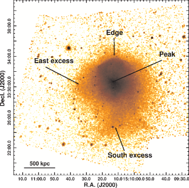
Refer to caption — Figure 1.— Combined, exposure-corrected and background-subtracted Chandra image in the $0.5-7.0\,$ keV energy band. The pixels are $1.968\arcsec$ on a side and the image has been smoothed with a Gaussian kernel with FWHM= $6\arcsec$ . Note the sharp edge to the north which we argue is a Mach $1.59$ shock.

As noted by kempner2003, to the south of the X-ray peak there is an extended region of low surface brightness emission which is $\sim 4$ ′ long. Our deeper data show that this low surface brightness emission is elongated with the axis of elongation pointing just east of south. Based on the fairly regular, diffuse morphology revealed by their shallower data, kempner2003 offered three explanations for this excess. Two of these explanations centred around the southern excess being associated with a smaller subcluster which is merging with A2034. The third and most favored explanation was that the south excess was due to the emission associated with a background cluster seen in projection through A2034. The highly elongated morphology, along with the lack of any clear galaxy association in the deeper SDSS images (Figure 2) indicate that the background cluster interpretation may be incorrect.

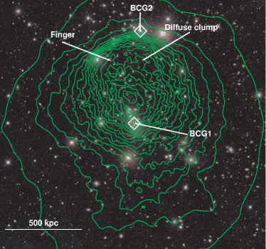
In Figure 2 we overlay contours from an adaptively smoothed Chandra image onto an SDSS RGB image. The peak in the X-ray emission is 172 kpc to the north of the BCG (hereafter, BCG1), while there does appear to be a less-prominent peak in the X-ray emission coincident with BCG1. Just north of the nose of the edge is another bright cluster member which we have labeled BCG2. Some $\sim 200$ kpc south of the nose is a diffuse clump of emission, while a finger of emission extends from the eastern portion of the edge toward the south. The deeper data also reveal a low surface brightness asymmetry $\sim 400\,$ kpc east of the peak in the X-ray brightness.

3.2. Temperature and Hardness ratio Maps

For the purpose of understanding the spectral properties of the ICM in A2034, we construct temperature and hardness ratio maps. The hardness ratio, defined here as the ratio of the flux in the $2-7$ keV and $0.5-7$ keV bands, does not produce a direct measure of the gas temperature. However, for a given number of source counts a hardness ratio map provides a simpler, higher signal-to-noise, model-independent diagnostic of the spectral properties in a region when compared with a single thermal component temperature map. Moreover, a hardness ratio map may reveal regions where a single component thermal model does not adequately describe the spectral properties of the ICM. Therefore, the hardness ratio and temperature maps can provide a complementary, quasi-independent, spatially resolved probe of the ICM spectral properties.

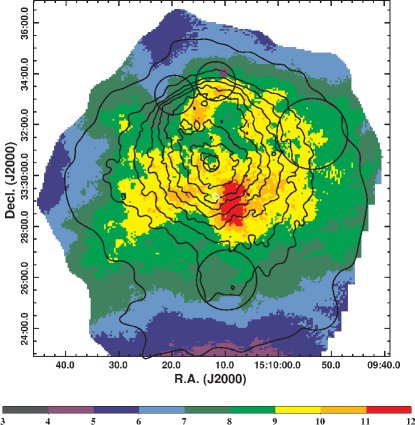
The temperature maps are generated in a similar manner to that described in randall2008 and are shown in the top left and top right panels of Figure 3. Briefly, each temperature map has pixels with a constant size ( $3.94\arcsec\times 3.94\arcsec$ ) and spectra for each pixel are extracted from a circular region with radius set such that the region contains a constant number of background subtracted 0.5-7 keV source counts. We produce a high spatial resolution map with 2000 source counts per extraction region, and a lower spatial resolution map with 8000 source counts per extraction region. The higher resolution temperature map provides a more accurate picture where there are abrupt changes in temperature, such as near shock and cold fronts. The lower resolution temperature map provides more accurate temperatures, particularly for the higher temperature regions, although it significantly smears out sharp gradients in temperature. For both maps, but more so the 8000 count map, in the low surface brightness regions the pixel values are correlated over large distances. To demonstrate this effect, we show extraction region sizes as black circles at five locations in the top left and top right panels of Figure 3.

Redistribution Matrix Files (RMFs) and Ancilliary Response Files (ARFs) are generated with the CIAO mkacisrmf and mkwarf tools, respectively. Because the RMFs can take several minutes to process, and because there are $\sim 200,000$ spectra to process, we extract the RMFs and ARFs on a more coarsely binned grid with $15.74\arcsec\times 15.74\arcsec$ pixels. The size of the extraction regions are generally much larger than the pixel size of this coarser grid, so the impact on the temperature measurements is small and well within the measurement uncertainties. The five spectra per pixel are fitted simultaneously in XSPEC (Version 12.7.1 arnaud1996) with an absorbed MEKAL model (mewe1985; mewe1986; Kaastra1992; liedahl1995). During the fitting the temperature is left as a free parameter which is tied across the spectra and the abundance is fixed at the global value $Z=0.33$ which is measured with respect to solar values (using ratios from anders1989). The normalizations are also left as free parameters, however for observations with similar pointings the values are tied together. Spectra are constrained to the energy range 0.7-7 keV, binned to contain at least one count per energy bin, and the modified Cash statistic, WSTAT, is minimized⁷⁷7heasarc.gsfc.nasa.gov/docs/xanadu/xspec/manual/
XSappendixStatistics.html.

The lower left panel of Figure 3 shows the upper confidence interval for the higher resolution, 2000 count, temperature map expressed as a fraction of the best fit temperature. The confidence intervals are measured at the $68\%$ level (corresponding to $\Delta(WSTAT)=1$ ) and are determined for a single parameter of interest. The confidence intervals are skewed about the best fit so that the upper confidence interval is generally a factor of $\sim 1.3$ higher than the lower confidence interval. Where the X-ray surface brightness is high, the upper confidence intervals are $10-15\%$ and $20-25\%$ of the best fit temperature for regions which have $kT<10$ keV and $kT>11$ keV, respectively. In the lower surface brightness regions, where the background flux begins to dominate, the relative uncertainties become much larger ( $>30\%$ ) where $kT>11$ keV. Given these uncertainties, regions with $kT<8\,$ keV are cooler than regions with $kT>10\,$ keV with $\gtrsim 90\%$ confidence.

Comparing the higher and lower resolution temperature maps, there is qualitative agreement on large scales. Clearly the distribution of temperatures is less patchy for the lower resolution, 8000 count, map and this is due to two main reasons. First, hot regions where $kT\gtrsim 11\,$ keV are less well constrained in the higher resolution, 2000 count, map and excursions to much higher temperatures on smaller scales may simply be due to statistical fluctuations which are not significant. The relative uncertainties on the lower resolution map are generally $<10\%$ and so the temperature map is considerably less noisy. Second, the large aperture required to collect 8000 counts smooths out real fluctuations in temperature which occur on scales smaller than the aperture. For example, the extraction region near the sharp edge to the north is roughly twice the diameter in the lower resolution map when compared with the higher resolution map (see the black circles in the top panels of Figure 3). Therefore, the temperature measurement on the brighter side of the edge is significantly contaminated by flux from the fainter side of the edge, washing out the sharp temperature gradient which is significant in the higher resolution map. For the remainder of this section, we focus our discussion around significant features seen in the higher resolution, 2000 count, map.

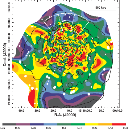
The lower right panel of Figure 3 shows the hardness ratio map. The map is produced by smoothing the background-subtracted and exposure-corrected 2-7 keV and 0.5-7 keV band images with a Gaussian kernel with an adaptive smoothing length. Rather than choosing an adaptive smoothing width based on one of the images (e.g., as in henning2009), we follow a similar method to that used in sanders2001. That is, we set the smoothing length such that the hardness ratio at each pixel has a relative uncertainty of $\sim 5\%$ . Comparison of the hardness ratio and temperature maps show that high temperature regions in the high resolution temperature map clearly map regions which are significantly harder in the hardness ratio map. This provides confidence that the regions with high temperature values in the 2000 count temperature map are regions with significantly harder, and likely hotter, emission. However, near the eastern portion of the edge there some differences between the high resolution temperature map and the hardness ratio map which we discuss below.

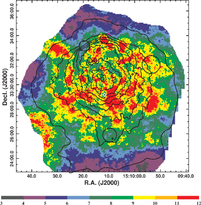
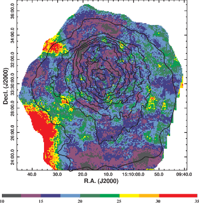
The distribution of temperatures is patchy and complicated and is broadly consistent with the map presented in kempner2003, although the deeper observations reveal several features associated with the northern edge which were not previously identified. The region corresponding to the nose of the northern edge has $kT\gtrsim 11$ keV and is significantly hotter than the ICM lying further north of the nose, which has $kT\simeq 6$ keV. This hotspot is highlighted by a black circle the radius of which shows the size of the extraction region there. While kempner2003 discuss a hot spot in the vicinity of the nose, it appears that the peak temperature in the hotspot seen in their Figure 7 lies somewhat further south and away from the nose. We confirm that the region discussed in kempner2003 is in fact hotter than its surrounds, but stress that it is separate from the hotspot detected at the nose. The sector of the edge lying to the west of the nose also shows a strong gradient in temperature in the sense that the temperature drops sharply going from the brighter side of the edge ( $\sim 9$ keV) to the fainter side ( $\sim 5-6$ keV). We note a second hot spot with $kT\gtrsim 12$ keV at the westernmost point of the edge. Thus, the nose and western sectors of the edge appear to harbour thermal properties which are more consistent with the edge being a shock front rather than a cold front.

In defining the position of the edge, kempner2003 appear to have focused on the sector just east of the nose. Figure 3 shows that the thermal properties of this eastern sector are somewhat abnormal. Near to the nose the temperature distribution is shock-like; inside the edge the temperature is $\simeq 9$ keV and drops abruptly to the north to $\simeq 7$ keV although there are several patches of hotter $\sim 8$ keV gas further ahead of the edge. These hotter $\simeq 8$ keV patches are also seen as a region of hard emission in the hardness ratio map. Following the edge further southeast, the temperature on the bright side of the edge drops abruptly to $6.5-7.5$ keV, similar to the temperature just outside the edge there. The constant temperature going from the inside to the outside of the edge does not appear to be consistent with the behavior expected of a shock or cold front. The hardness ratio map shows a finger of emission which starts at the edge and extends to the south. This finger is significantly softer than the surrounding ICM. The hardness ratio map has better spatial resolution than the temperature map, and it shows that this soft finger does not follow the surface brightness contours which trace the edge. The nature of this soft finger of emission is unclear, but it is likely responsible for the odd behaviour observed in the temperature map near the eastern portion of the edge. Since projection effects and cross contamination of emission from either side of the edge may wash out temperature gradients at the edge, we will investigate the profile across the edge further in Section 3.3 using well-defined regions inside and outside the edge.

Aside from the edge, there are several other features of note in the temperature map. As noted in kempner2003, the temperature at the peak in the X-ray surface brightness is cooler than its surrounds. To the south of the peak in the X-ray surface brightness is a band of hot $\gtrsim 11$ keV gas that extends $\sim 750$ kpc along an east-west axis (similar to the hot region seen just west of the main cluster in the Bullet; owers2009c). Embedded within this hot band is a region of enhanced surface brightness and cooler $kT\simeq 7.5$ keV gas which is spatially coincident with BCG1 (open white diamond symbol in the left panel of Figure 3). Further south, the temperature maps show that the extended region of low surface brightness emission discussed in Section 3.1 harbors cooler $\sim 6.5-7.5$ keV gas. At large radii, the temperature of the gas is generally much cooler than the central regions and has $kT\lesssim 5$ keV.

3.3. Profiles across the edge

3.3.1 Surface brightness profile

As a first step toward understanding the physical nature of the northern edge, we examine the surface brightness profile in that region with the aim of measuring the density jump at the edge. To that end we import the broken powerlaw density model (described in detail in owers2009c) into the Sherpa package and fit to the 0.5-7 keV image near the edge. Initially, we fit to an annular sector centered at R.A.=15:10:11.93, decl. = 33:30:36.77 and with an angular range $50-130\arcdeg$ , where angles are measured north from west. The sector is shown as a white dashed region in the right panel of Figure 3. The center is chosen as the approximate center of the radius of curvature of the edge, while the opening angle is chosen to match the range over which the edge is clearly visible. Given the complicated surface brightness distribution away from the edge and toward the cluster centre, and the limited accuracy of the powerlaw model approximation to the data at larger radii, we also constrain the radial range of the data fitted to $147\arcsec<r<276\arcsec$ . Because of the low counts per pixel, during fitting we minimize the CSTAT statistic and use a combination of Monte-Carlo and simplex methods for the minimization. We fit for the powerlaw slopes and amplitudes, the position of the edge and the ellipticity. The centroid of the model is fixed to the initial estimate of the center of curvature of the front, while the position angle is set to $90\arcdeg$ to bisect the edge. A constant is added to the broken powerlaw model to account for the background. The best fitting values and their associated uncertainties are presented in Table 2. The density jump across the edge is well approximated as the square root of the ratio of the surface brightness amplitudes just inside, $A_{1}$ , and outside, $A_{2}$ , the edge, as determined during the fitting (owers2009c). This gives a density jump of $1.72^{+0.05}_{-0.04}$ .

Table 2Parameters for the best fitting density models to the surface brightness across the northern edge.

Sector	Centroid	$\theta$ ( $\Delta\theta$ )	$R_{\rm f}$	Ellipticity	$\alpha_{1}$	$\alpha_{2}$	$A_{1}$	$A_{2}$	$\sqrt{A_{1}/A_{2}}$
	(J2000)	(degrees)	(kpc)				( $10^{-8}$ )	( $10^{-8}$ )
Total	15:10:11.93, 33:30:36.77	90 (50-130)	$402.0^{+0.4}_{-0.8}$	$0.14^{+0.01}_{-0.01}$	$1.50^{+0.10}_{-0.11}$	$2.32^{+0.07}_{-0.07}$	$7.30^{+0.22}_{-0.19}$	$2.46^{+0.12}_{-0.11}$	$1.72^{+0.05}_{-0.04}$
Nose	15:10:11.93, 33:30:36.77	90 (76.67-103.33)	$404.4^{+0.9}_{-1.4}$	$0.29^{+0.02}_{-0.04}$	$1.14_{-0.15}^{+0.15}$	$2.30_{-0.13}^{+0.13}$	$8.02^{+0.34}_{-0.32}$	$2.40^{+0.21}_{-0.18}$	$1.83^{+0.09}_{-0.08}$
East	15:10:09.73, 33:30:17.07	116.67 (103.33-130)	$447.4^{+0.5}_{-1.7}$	$0.00^{----}_{----}$	$1.61_{-0.32}^{+0.23}$	$2.57_{-0.16}^{+0.13}$	$9.93^{+0.71}_{-0.45}$	$2.85^{+0.29}_{-0.20}$	$1.86^{+0.12}_{-0.08}$
West	15:10:11.93, 33:30:36.77	63.33 (50-76.67)	$391.6^{+1.1}_{-2.0}$	$0.00^{----}_{----}$	$1.32^{+0.23}_{-0.27}$	$2.26_{-0.13}^{+0.14}$	$6.03^{+0.48}_{-0.35}$	$2.17_{-0.18}^{+0.23}$	$1.67^{+0.11}_{-0.08}$

Note. — $R_{\rm f}$ is the position of the edge. The East and West sectors have ellipticity fixed to zero. The $\alpha_{1}$ and $\alpha_{2}$ values are the powerlaw slopes inside and outside the edge, respectively. The $A_{1}$ and $A_{2}$ values give the surface brightness just inside and just outside the edge, respectively, and they have units ${\rm photons/cm^{2}/s/pixel}$ where one pixel is $1.968\arcsec\times 1.968\arcsec$ . For a detailed description of the density model, see owers2009c.