Skew and implied leverage effect: smile dynamics revisited

Abstract

We revisit the “Smile Dynamics” problem, which consists in relating the implied leverage (i.e. the correlation of the at-the-money volatility with the returns of the underlying) and the skew of the option smile. The ratio between these two quantities, called “Skew-Stickiness Ratio” (SSR) by Bergomi Ber2 , saturates to the value $2$ for linear models in the limit of small maturities, and converges to $1$ for long maturities. We show that for more general, non-linear models (such as the asymmetric GARCH model), Bergomi’s result must be modified, and can be larger than $2$ for small maturities. The discrepancy comes from the fact that the volatility skew is, in general, different from the skewness of the underlying. We compare our theory with empirical results, using data both from option markets and from the underlying price series, for the S&P500 and the DAX. We find, among other things, that although both the implied leverage and the skew appear to be too strong on option markets, their ratio is well explained by the theory. We observe that the SSR indeed becomes larger than $2$ for small maturities.

I Introduction

Among the best known “stylized facts” about option smiles are a) their skew, i.e. the fact that downstrike volatilities are generally higher than upstrike volatilities, reflecting the anticipated negative skewness of market moves and b) the “implied leverage effect”, i.e. the tendency of at-the-money volatilities to increase when the underlying market goes down. A huge amount of effort has been devoted to building a theoretical framework that accounts quantatively for these features (see e.g. BaFo ; BP ; SABR ; Bergomi ). Simple “rules of thumb” are used by market makers in order to relate these two effects. One of them is the “sticky strike” rule, which assumes that the implied volatility of an option only depends on its strike $K$. Assuming the smile to be locally linear around the money, one defines:

$$\sigma_{{\rm BS},T}(K)\approx\sigma_{{\rm{ATM}},T}\left[1+\text{Skew}_{T}\,\mathcal{M}\right],\quad{\mbox{where}}\quad\mathcal{M}=\frac{\ln(K/S)}{\sigma_{{\rm{ATM}},T}\sqrt{T}}\ll 1,$$ (I.1)

and $\sigma_{{\rm{ATM}},T}=\sigma_{{\rm BS},T}(K=S)$ is the “at-the-money” implied volatility, $T$ the maturity, $\mathcal{M}$ is the rescaled moneyness, assumed to be small, and $\text{Skew}_{T}$ is the relative slope of the smile, that we will call throughout the “skew”. Assuming “sticky strike” as defined above therefore immediately leads to the following relation between the change of $\sigma_{{\rm{ATM}},T}$ and the skew:

$$\delta\sigma_{{\rm BS},T}(K)=0=\delta\sigma_{{\rm{ATM}},T}+\text{Skew}_{T}\,\frac{\delta S}{S\sqrt{T}}\longrightarrow\delta\sigma_{{\rm{ATM}},T}=-\text{Skew}_{T}\frac{\delta S}{S\sqrt{T}}.$$ (I.2)

More generally, L. Bergomi Ber2 proposed to introduce the (maturity dependent) Skew-Stickiness Ratio (SSR) $R_{T}$ defined as:

$$\delta\sigma_{{\rm{ATM}},T}:=-R_{T}\,\text{Skew}_{T}\,\frac{\delta S}{S\sqrt{T}},$$ (I.3)

with $R_{T}\equiv 1$ if the above “sticky strike” rule holds, and $R_{T}\equiv 0$ for the so-called “sticky delta” rule, where the volatility only depends on the moneyness (and is thus trivially constant at the money, for $\mathcal{M}=0$). The definition of $R_{T}$ in (I.3) should be understood in the sense of a standard regression of $\delta\sigma_{{\rm{ATM}},T}$ against ${\delta S}/{S}$.

Can these rules be given some theoretical foundation, and what value of $R_{T}$ should one expect? Recently, Bergomi Ber2 and Ciliberti-Bouchaud-Potters CBP ; CBP-E independently and using a slightly different framework, proposed a theory for $R_{T}$ and compared the results with empirical data. Bergomi assumes a general linear model for the forward volatility dynamics and expands to lowest order in vol-of-vol, whereas Ciliberti et al. use a cumulant expansion for the smile. The two results coincide and provide the following expression for the SSR :

$$R_{T}=\frac{\sum_{\ell=1}^{T}g_{L}(\ell)}{\sum_{\ell=1}^{T}(1-\frac{\ell}{T})g_{L}(\ell)},$$ (I.4)

where $g_{L}(\ell)$ is the so-called leverage correlation function of the underlying price process BMP ; BP ; CBP :

$$g_{L}(\ell)=\frac{E[r_{i}r_{i+\ell}^{2}]}{\sigma^{3}},$$ (I.5)

where $r_{i}$ is the return at time $i$ and $\sigma^{2}=E[r_{i}^{2}]$ the average square volatility of the process. It is interesting to give an explicit expression for $R_{T}$ in the case where $g_{T}(\ell)$ is a simple exponential function $-A\exp(-\ell/\tau)$ with a relaxation time $\tau$. This shape is actually not a bad approximation for major stock indices, with $A\sim 0.2$ and $\tau\sim 30-50$ days CBP . The SSR then takes the following form:

$$R_{T}\approx\frac{T(1-e^{-T/\tau})}{T-\tau(1-e^{-T/\tau})},\qquad(\tau\gg 1),$$ (I.6)

which displays the following limits: $R_{T}\approx 2$ ($1\ll T\ll\tau$) and $R_{T}\approx 1+\tau/T$ ($T\gg\tau$). As shown in Bergomi Ber2 , these limiting values are in fact independent of $g_{L}(\ell)$, provided it decays fast enough for large $\ell$. Note however that for $\tau=50$ days and $T=250$ days (1 year of trading), $R_{T}\approx 1.25$ still substantially larger than unity.

These results are interesting, but the framework within which they were obtained turns out to be restrictive, for several reasons. First, as shown in DVCB , the cumulant expansion for the smile (and hence the theoretical approximation for the skew $\text{Skew}_{T}$) is very inaccurate in practice. An alternative, general smile formula, without any assumption on the underlying model (except the existence of all moments of order $\;\leqslant\;2$ for the returns) was derived in DVCB . One of the salient features of this new formula is that the coefficients of the quadratic expansion involve low moments of the return distribution which do not necessarily coincide with the coefficients given by a standard cumulant expansion. Second, the class of linear models considered by Bergomi Ber2 and Bergomi & Guyon BG cannot handle the strong, non-linear leverage effect that seems to characterize stock index returns. The main purpose of this paper is to show that one can derive analytically the skew term of the expansion within a large class of non linear Gaussian models. We specialize our general results to the case of the totally assymetric GARCH model, which is believed to provide a good description of the (non-linear) leverage effect of stock indices. We finally compare our theoretical results with empirical data and comment on the remaining discrepancies.

II Main theoretical results

II.1 The framework

Similarly to Bergomi , we choose to model the full forward variance curve $\{v_{i}^{i+\ell}\}_{\ell\;\geqslant\;0}$ directly. This approach is general and flexible as it does not assume any shape for the instantaneous forward variance curve; in particular, one can either choose to calibrate the model on the market forward variance curve (using the options market) or assume some form for the forward variance curve using either historical data or an underlying variance model. We introduce a sequence $(\epsilon_{i})_{i\in\mathbb{Z}}$ of i.i.d. standard Gaussian variables and an arbitrary function $f$ that satisfies $E[f(\epsilon_{i})]=0$. Let $\mathcal{F}_{i}=\sigma\{\epsilon_{j};\>j\;\leqslant\;i\}$ be the relevant filtration. We adopt the following framework for the (log) price $S_{i}$:

$$r_{i}:=\ln\frac{S_{i+1}}{S_{i}}=\sigma_{i}\>\epsilon_{i},\quad v_{i+1}^{i+\ell}-v_{i}^{i+\ell}=\nu\lambda_{i}^{i+\ell}(\{v_{i}^{u}\}_{u\;\geqslant\;i})f(\epsilon_{i})$$ (II.1)

where $v_{i}^{i+\ell}=E\left[\sigma_{i+\ell}^{2}|\mathcal{F}_{i-1}\right]$ is the forward variance (with $\sigma_{i}^{2}\equiv v_{i}^{i}$), $\nu$ is an expansion parameter (the vol of vol) and the set of $\lambda_{i}^{i+\ell}(\{v_{i}^{u}\}_{u\;\geqslant\;i})$ are arbitrary functions that describe the coupling of the variance curve with the current residual return $\epsilon_{i}$, that may themselves depend on the current forward variance curve $\{v_{i}^{u}\}_{u\;\geqslant\;i}$. The initial ($t=1$) variance curve is $v_{1}^{j}$, $j\;\geqslant\;1$, and the total expected variance up to maturity is $V_{T}=\sum_{j=1}^{T}v_{1}^{j}$. In the linear case, i.e. $f(x)=x$, we recover (in a discrete setting) the framework of Bergomi & Guyon BG . In the sequel, we will restrict to a first order expansion in $\nu$ as we focus in this paper on the skew term in the smile expansion (I.1). Within this approximation, the functions $\lambda_{i}^{i+\ell}$ are functions of the initial (deterministic) curve $v_{1}^{j}$. We will make this dependence implicit, as this lightens the notations.

Note that since the $\epsilon_{i}$ are i.i.d Gaussian variables with $E[f(\epsilon_{i})]=0$, one deduces the following equality, that relates $\lambda_{i}^{i+\ell}$ to the leverage correlation function:

$$E[r_{i}r_{i+\ell}^{2}]=\nu\sqrt{v_{i}^{i}}\lambda_{i}^{i+\ell}E[f^{\prime}(\epsilon_{i})].$$ (II.2)

II.2 The smile formula

We get the following smile formula at order 1 in $\nu$ (see proof in the appendix):

$$\sigma_{{\rm BS},T}=\sqrt{\frac{V_{T}}{T}}+\frac{\nu}{2\sqrt{V_{T}T}}\sum_{i=1}^{T}\sum_{j=1}^{i-1}\lambda_{j}^{i}E\left[f\left(\frac{\sqrt{v_{1}^{j}}}{V_{T}}\left(\ln\left(\frac{K}{S}\right)+\frac{V_{T}}{2}\right)+Y_{j}\right)\right]$$ (II.3)

where $Y_{j}$ a centered gaussian variable of variance $E[Y_{j}^{2}]=1-v_{1}^{j}/V_{T}$.

We therefore get the following smile expansion at order $1$ in $\nu$ and in the modified rescaled moneyness $\mathcal{M}:=(\ln(K/S)+\frac{V_{T}}{2})/\sigma_{{\rm{ATM}},T}\sqrt{T}$:

$$\sigma_{{\rm BS},T}=\sigma_{{\rm{ATM}},T}\left[1+\text{Skew}_{T}\mathcal{M}\right],\qquad\sigma_{{\rm{ATM}},T}\equiv\sqrt{\frac{V_{T}}{T}},$$ (II.4)

where the skew is given by the general expression

$$\text{Skew}_{T}=\frac{\nu}{2V_{T}^{3/2}}\sum_{i=1}^{T}\sum_{j=1}^{i-1}\sqrt{v_{1}^{j}}\lambda_{j}^{i}E[f^{\prime}(Y_{j})]$$ (II.5)

Note that our method in fact enables one to derive a smile formula to quadratic order in $\mathcal{M}$ and to second order in $\nu$. For the sake of simplicity, we do not write the corresponding (cumbersome) expressions here. However, in the linear case $f(x)=x$, we recover exactly the formulae of Bergomi-Guyon BG established in a continuous setting, by working on a time step $\delta t$ and then taking the limit as $\delta t\to 0$.

II.3 Skew and Skewness

Recall that using a standard cumulant expansion one derives the following smile formula (BaFo ; BCP ; BP ):

$$\sigma_{{\rm BS}}=\sigma_{{\rm{ATM}},T}\left[1+\frac{\mathcal{S}_{T}}{6}\mathcal{M}\right],\qquad\sigma_{{\rm{ATM}},T}\equiv\sqrt{\frac{V_{T}}{T}},$$ (II.6)

where $\mathcal{S}_{T}$ is the skewness of $\ln(S_{T}/S_{1})$, i.e. the return between now and maturity. Within the present framework, the skewness at order 1 in $\nu$ can be computed as:

$$\frac{\mathcal{S}_{T}}{6}=\frac{\nu}{2V_{T}^{3/2}}\left(\sum_{i=2}^{T}\sum_{j=1}^{i-1}\sqrt{v_{1}^{j}}\lambda_{j}^{i}\right)E[f^{\prime}(\epsilon)],$$ (II.7)

which is close to, but different from, the formula above for the skew $\text{Skew}_{T}$. However, for a linear model where $f^{\prime}(x)\equiv 1$, the two formulas exactly coincide. To first order in $\nu$, the skewness of the returns and the skew of the smile are therefore identical for a general linear model:

$$f(x)=x\longrightarrow\text{Skew}_{T}\equiv\frac{\mathcal{S}_{T}}{6}.$$ (II.8)

II.4 The implied leverage coefficient and the SSR

One can also readily compute the implied leverage within our general non-linear model. The difference between tomorrow’s volatility and today’s volatility for ATM options of maturity $T$ is given by:

$$\frac{1}{T}\delta V_{T}=\frac{1}{T}\left[\sum_{j=2}^{T+1}v_{2}^{j}-\sum_{j=1}^{T}v_{1}^{j}\right]=\frac{1}{T}(v_{1}^{T+1}-v_{1}^{1})+\frac{\nu f(\epsilon_{1})}{T}\left[\sum_{j=2}^{T+1}\lambda_{1}^{j}\right]$$ (II.9)

Using $\delta V_{T}=2T\sigma_{{\rm{ATM}},T}\,\delta\sigma_{{\rm{ATM}},T}$, $E[r_{1}f(\epsilon_{1})]\equiv\sigma_{1}E[f^{\prime}(\epsilon_{1})]$ and integration by parts for the Gaussian variable $\epsilon_{1}$ , we finally deduce a formula for the implied leverage $\gamma_{T}$, i.e. the correlation between the return and the change of implied ATM volatility as:

$$\gamma_{T}:=\frac{E[\delta\sigma_{{\rm{ATM}},T}\cdot r_{1}]}{E[r_{1}^{2}]}=\frac{\nu E[f^{\prime}(\epsilon_{1})]}{2\sqrt{T\sigma_{1}^{2}V_{T}}}\left[\sum_{j=2}^{T+1}\lambda_{1}^{j}\right].$$ (II.10)

where we have used $E(\epsilon_{1})=0$. Here, we have neglected any drift effect, which is reasonable for option pricing in a risk neutral framework.

The average SSR is defined, consistently with Eq. (I.3), as:

$${R_{T}}:=\frac{\gamma_{T}\sqrt{T}}{\text{Skew}_{T}}.$$ (II.11)

In a linear model where skew and skewness are identical (up to a factor $6$), the final expression for the SSR is therefore given by:

$$\left.\widehat{R}_{T}\right|_{lin.}=\frac{V_{T}}{\sigma_{1}}\frac{\sum_{j=2}^{T+1}\lambda_{1}^{j}}{\sum_{i=2}^{T}\sum_{j=1}^{i-1}\sqrt{v_{1}^{j}}\lambda_{j}^{i}},$$ (II.12)

which is precisely Bergomi’s result in a discrete time setting Ber2 . Note that for a flat forward variance curve and for a time-translation invariant model, one has $v_{1}^{j}=v_{1}^{1}\equiv\sigma_{1}^{2}$, $V_{T}=Tv_{1}^{1}$, and $\lambda_{j}^{i}\propto g_{L}(j-i)$ where $g_{L}$ is the leverage correlation function introduced above. In this case, one recovers exactly Eq. (I.4) above.

However, in the general case, ${R}_{T}$ is not given by the above expression, but is corrected by a factor that accounts for the difference between the skew and the skewness:

$${R_{T}}=\left.\widehat{R}_{T}\right|_{lin.}\times\frac{\mathcal{S}_{T}/6}{\text{Skew}_{T}}.$$ (II.13)

We will study below this correction factor, both within the asymmetric GARCH model and using empirical data.

Note finally that using Eq. (II.2), the implied leverage can alternatively be re-written in terms of the leverage correlation function as:

$$\gamma_{T}=\frac{1}{2\sqrt{T\sigma_{1}^{4}V_{T}}}\left[\sum_{j=2}^{T+1}E[r_{1}r_{j}^{2}]\right],$$ (II.14)

or, for a flat forward variance curve;

$$\gamma_{T}=\frac{1}{2T\sigma_{1}^{3}}\left[\sum_{j=2}^{T+1}E[r_{1}r_{j}^{2}]\right].$$ (II.15)

In fact, expressions (II.14) and (II.15) for $\gamma_{T}$ are quite general and valid in a much more general setting than the one we consider here; indeed, they do not rely on any modelling assumption for the returns $r_{i}$.

III The asymmetric GARCH model

In order to give some flesh to the above formulae in the context of an empirically relevant, non-linear model for price changes, we consider the following so-called fully asymmetric GARCH model:

$$r_{i}=\sigma_{i}\epsilon_{i},\quad\sigma_{i+1}^{2}=v_{0}^{2}+\rho(\sigma_{i}^{2}-v_{0}^{2})+\nu\sigma_{i}^{2}\left(\epsilon_{i}^{2}1_{\epsilon_{i}<0}-\frac{1}{2}\right)$$ (III.1)

where $(\epsilon_{i})_{i\in\mathbb{Z}}$ are i.i.d. standard Gaussian random variables. In the notation above, one has $f(x)=x^{2}1_{x<0}-1/2$.

We set $\sigma_{i}^{2}=v_{0}^{2}(1+\mathcal{X}_{i})$, so that the above is equivalent to the following recursion

$$\mathcal{X}_{i+1}=\rho\mathcal{X}_{i}+\nu(1+\mathcal{X}_{i})(\epsilon_{i}^{2}1_{\epsilon_{i}<0}-\frac{1}{2})$$ (III.2)

By iterating the above expression, we get the following exact expression for $\sigma_{i}^{2}$ ($i\;\geqslant\;2$):

$$\sigma_{i}^{2}=v_{0}^{2}(1+\rho^{i-1}\mathcal{X}_{1})+\nu\sum_{j=1}^{i-1}\rho^{i-1-j}\sigma_{j}^{2}\left(\epsilon_{j}^{2}1_{\epsilon_{j}<0}-\frac{1}{2}\right)$$ (III.3)

Therefore, to first order in $\nu$, we get, for arbitrary $j$ and $i$ with $j-i\;\geqslant\;1$:

$$\sigma_{j}^{2}=v_{0}^{2}(1+\rho^{j-i}\mathcal{X}_{i})+\nu V_{0}^{2}\sum_{k=i}^{j-1}\rho^{j-1-k}(1+\rho^{k-i}\mathcal{X}_{i})\left(\epsilon_{k}^{2}1_{\epsilon_{k}<0}-\frac{1}{2}\right)$$ (III.4)

which leads to the following expression for the forward variance curve

$$v_{i}^{j}=E[\sigma_{j}^{2}|\mathcal{X}_{i}]=v_{0}^{2}(1+\rho^{j-i}\mathcal{X}_{i})$$ (III.5)

To first order in $\nu$, we also obtain:

$$v_{i+1}^{j}-v_{i}^{j} =\nu v_{0}^{2}\rho^{j-i-1}(1+\mathcal{X}_{i})\left(\epsilon_{i}^{2}1_{\epsilon_{i}<0}-\frac{1}{2}\right)$$

$$=\frac{\nu}{\rho}(v_{0}^{2}(\rho^{j-i}-1)+v_{i}^{j})\left(\epsilon_{i}^{2}1_{\epsilon_{i}<0}-\frac{1}{2}\right)$$

Therefore, we finally obtain for the $\lambda_{i}^{j}$ (which indeed explicitly depend on the forward rate):

$$\lambda_{i}^{j}=\frac{1}{\rho}(v_{0}^{2}(\rho^{j-i}-1)+v_{i}^{j})$$ (III.6)

Finally, since $f^{\prime}(x)=2x1_{x<0}$, we get the following expression for the skew and the skewness :

$$\text{Skew}_{T} =-\sqrt{\frac{2}{\pi}}\frac{\nu}{2V_{T}^{3/2}}\sum_{j=2}^{T}\sum_{i=1}^{j-1}\sqrt{v_{1}^{i}}\lambda_{i}^{j}\sqrt{1-\frac{v_{1}^{i}}{V_{T}}}$$

$$=-\sqrt{\frac{2}{\pi}}\frac{\nu v_{0}^{3}}{2V_{T}^{3/2}}\sum_{j=2}^{T}\sum_{i=1}^{j-1}\sqrt{1+\rho^{i-1}\mathcal{X}_{1}}(\rho^{j-i-1}+\rho^{j-2}\mathcal{X}_{1})\sqrt{1-\frac{v_{1}^{i}}{V_{T}}}$$

and

$$\frac{\mathcal{S}_{T}}{6} =-\sqrt{\frac{2}{\pi}}\frac{\nu}{2V_{T}^{3/2}}\sum_{j=2}^{T}\sum_{i=1}^{j-1}\sqrt{v_{1}^{i}}\lambda_{i}^{j}$$

$$=-\sqrt{\frac{2}{\pi}}\frac{\nu v_{0}^{3}}{2V_{T}^{3/2}}\sum_{j=2}^{T}\sum_{i=1}^{j-1}\sqrt{1+\rho^{i-1}\mathcal{X}_{1}}(\rho^{j-i-1}+\rho^{j-2}\mathcal{X}_{1})$$

Here, the variance $V_{T}$ is given by:

$$V_{T} =\sum_{i=1}^{T}v_{1}^{i}=v_{0}^{2}\left(T+\frac{1-\rho^{T}}{1-\rho}\mathcal{X}_{1}\right),$$

therefore leading to the following skewness/skew ratio:

$$\frac{\mathcal{S}_{T}/6}{\text{Skew}_{T}}=\frac{\sum_{j=2}^{T}\sum_{i=1}^{j-1}\sqrt{1+\rho^{i-1}\mathcal{X}_{1}}(\rho^{j-i-1}+\rho^{j-2}\mathcal{X}_{1})}{\sum_{j=2}^{T}\sum_{i=1}^{j-1}\sqrt{1+\rho^{i-1}\mathcal{X}_{1}}(\rho^{j-i-1}+\rho^{j-2}\mathcal{X}_{1})\sqrt{1-\frac{1+\rho^{i-1}\mathcal{X}_{1}}{T+\frac{1-\rho^{T}}{1-\rho}\mathcal{X}_{1}}}}$$ (III.7)

This expression drastically simplifies when the initial volatility is equal to the average volatility, i.e. $\mathcal{X}_{1}=0$. In this case, one simply obtains:

$$\frac{\mathcal{S}_{T}/6}{\text{Skew}_{T}}=\sqrt{\frac{T}{T-1}},$$ (III.8)

which is equal to $2$ for $T=2$ and tends to unity when $T\to\infty$. We see clearly that in this model, the skew is systematically smaller than its third cumulant estimate, i.e. the skewness. Dividing by the skewness instead of the skew therefore leads to an underestimate of the “true” SSR. Finally, the implied leverage is given by:

$$\gamma_{T}\approx-\frac{\nu\sqrt{1+\mathcal{X}_{1}}}{\sqrt{2\pi}\sqrt{T(T+\frac{1-\rho^{T}}{1-\rho}\mathcal{X}_{1})}}\frac{1-\rho^{T}}{1-\rho}.$$ (III.9)

IV Data analysis: skew, skewness and SSR

The central result of our paper is given by Eqs. (II.12, II.13), that relates Bergomi’s Skew-Stickiness Ratio (SSR) $R_{T}$ to empirically measurable quantities. The three questions we want to address here are:

1. How well does our central result Eq. (II.13) account for the SSR of index option markets?

2. How strong is the correction factor $\mathcal{S}_{T}/6\,\mathrm{Skew}_{T}$, induced by non-linear effects?

3. How well are these features reproduced by the (non-linear) asymmetric GARCH model investigated in the above section?

In order to discuss these issues, we need data both from the option markets and from the underlying contract. We have focused on two markets, S&P 500 index and DAX, for which we have full information on both the underlying and on the option smiles for various maturities. Our data set runs from 2000 to 2013 for the S&P 500 and from 2002 to 2013 for the DAX.

We extract from the data various statistical quantities.

1. From the historical returns $r_{i}$ of the underlying index, we measure:

   • The leverage correlation function $g_{L}(\ell)$, obtained as a time average of the ratio $r_{i}r_{i+\ell}^{2}/\sigma_{i}^{3}$, where $\sigma_{i}^{2}$ is a 20 day exponential moving average (EMA) of the past squared returns.

   • A low moment estimator of the skewness of the distribution of returns over $T$ days, defined as:

     $$\beta_{T}=\sqrt{\frac{\pi}{2}}\left[1-2P(\widetilde{r}_{T}>0)\right],$$ (IV.1)

     where $\widetilde{r}_{T}$ is the detrended T-day return and $P(\widetilde{r}_{T}>0)$ is the probability that $\widetilde{r}_{T}$ is positive. We determined the local drift using an EMA filter with timescale $T=1000$ days.

   It turns out that the skew of the smile, $\text{Skew}_{T}$, should be on average equal to $\beta_{T}$ for fairly priced options DVCB . Moreover, the standard skewness of the returns, $\mathcal{S}_{T}$, can be obtained from the leverage correlation function as BP

   $$\mathcal{S}_{T}=\frac{\zeta_{1}}{\sqrt{T}}+\frac{3}{\sqrt{T}}\sum_{\ell=1}^{T}\left(1-\frac{\ell}{T}\right)g_{L}(\ell)$$ (IV.2)

   where $\zeta_{1}$ is the skewness of daily returns.

2. From option prices we extract the volatility smile for different moneyness and maturities, which allows us to measure:

   • The skew of the smile $\text{Skew}_{T}$, defined from Eq. (I.1), that we average over the whole time period, for a set of fixed maturities.

   • The implied leverage coefficient $\gamma_{T}$, measured as the regression coefficient of the changes of ATM implied vol on the returns of the underlying.

   • Finally, Bergomi’s SSR is obtained as the time-averaged local SS Ratio, measured as:

     $$\widehat{\mathcal{R}}_{T}(t;M)=M\frac{\sum_{i=t-M}^{t}\left(\sigma_{{\rm{ATM}},T}(i+1)-\sigma_{{\rm{ATM}},T}(i)\right)\times r_{i}}{\sum_{i=t-M}^{t}\text{Skew}_{T}(i)\times\sum_{i=t-M}^{t}r_{i}^{2}}$$ (IV.3)

     where $M=50$ is the size of the moving average window. Our empirical estimate of the SSR is then obtained as:

     $${\mathcal{R}}_{T}=\langle\widehat{\mathcal{R}}_{T}(t;M)\rangle_{t}.$$ (IV.4)

In order to compare $\gamma_{T}$ and ${\mathcal{R}}_{T}$ with theoretical estimates, we furthermore assume that the underlying process is time-translation invariant and that the forward variance is flat on average, which allows us to obtain $\gamma_{T}$ from Eq. (II.15) CBP-E :

$$\gamma_{T}^{th.}\approx\frac{1}{2T}\sum_{\ell=1}^{T}g_{L}(\ell).$$ (IV.5)

Our results are summarized in three figures, each showing data for the S&P 500 (left) and DAX (right).

• In Fig. 1-a,b, we show as a function of the maturity $T$ the unconditional skew $\text{Skew}_{T}$ and unconditional implied leverage $\gamma_{T}$, both extracted from option data, which we compare with their theoretical estimates, $\beta_{T}$ and $\gamma_{T}^{th.}$, obtained using the historical returns of the underlying. We conclude that (a) the options skews on the S&P index are stronger than predicted by $\beta_{T}$, but match very well for the DAX; (b) the implied leverage $\gamma_{T}$ of S&P options is well estimated for short maturies, but systematically too strong for larger maturities, as observed in CBP-E . For the DAX, on the other hand, the implied leverage $\gamma_{T}$ appears to be too weak for short maturities and too strong for large maturities.

• In Fig. 2-a,b, we show Bergomi’s SSR $R_{T}$ as a function of maturity, together with our theoretical estimate $R_{T}^{th.}=\gamma_{T}^{th.}\sqrt{T}/\beta_{T}$, based either on the historical returns (using Eq. IV.5) or on the predictions based on the asymmetric GARCH model, itself calibrated on historical returns . We find that the overall agreement is quite good, in particular with the predictions of the asymmetric GARCH model which are less noisy than the direct estimate based on historical returns. Therefore, although both the implied leverage $\gamma_{T}$ and the skew $\text{Skew}_{T}$ appear to be too strong on option markets, their ratio is about right! Still, observe that $R_{T}$ clearly becomes larger than the asymptotic Bergomi value $2$ for small maturities. This is due to the correction factor $(\mathcal{S}_{T}/6)/\text{Skew}_{T}>1$ that appears in Eq. (II.13), to which we turn next.

• In Fig 3-a,b, we now plot the expected value of the correction factor $(\mathcal{S}_{T}/6)/\text{Skew}_{T}$ as a function of maturity, again using either a direct estimate based on Eqs. (IV.1), (IV.2), or on the prediction of the asymmetric GARCH model with empirically calibrated parameters. We see that in the case of the S&P 500 the value of this ratio is overall not very well captured by the GARCH model, which underestimates this ratio, as already noticed in DVCB . One of the known weaknesses of the GARCH model is that it fails to capture the long-range memory of the volatility process. This might explain part of the discrepancy seen here. In the case of the DAX, the ratio is much closer to unity (except for small maturities where it is below $1$), suggesting that non-linear effects are weaker in this case.

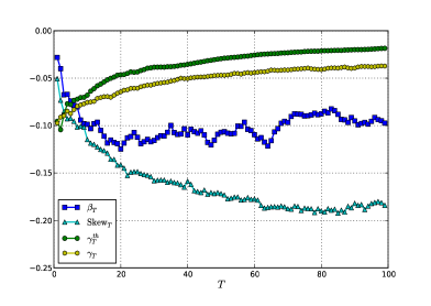
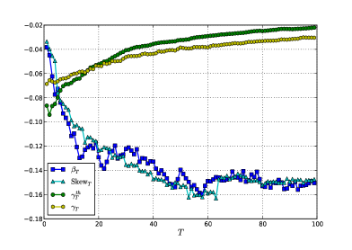
Figure 1: Comparison between theoretical prediction of the unconditional values of $\mathrm{Skew}_{T}$ and of $\gamma_{T}$, and their estimation based on option data. The left panel shows the result for S&P 500 whereas the right panel is for DAX.

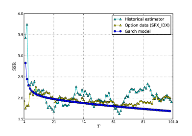
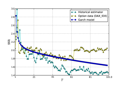
Figure 2: Comparison between the real SSR estimated with option data as $\gamma_{T}\sqrt{T}/\mathrm{Skew}_{T}$ and the theoretical prediction based on historical data, $\gamma_{T}^{th.}\sqrt{T}/\beta_{T}$. The left panel shows the result for S&P 500 whereas the right panel is for DAX.

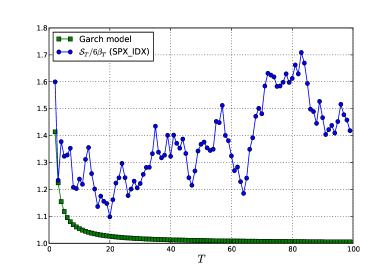
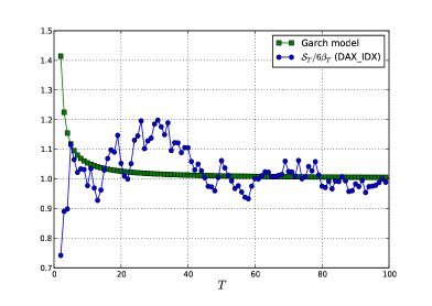
Figure 3: Comparison between $(\mathcal{S}_{T}/6)/\mathrm{Skew}_{T}$ estimated with S&P 500 data and the prediction of GARCH model for S&P 500 (left panel) and DAX (right panel).

V Conclusion

In this paper, we have revisited the problem of the dynamics of smiles, as envisaged in Ber2 ; CBP ; CBP-E , which consists in relating the “implied leverage” (i.e. the correlation of the at-the-money volatility with the returns of the underlying) and the skew of the option smile. As noticed by Bergomi Ber2 , the ratio between these two quantities, dubbed the “Skew-Stickiness Ratio” (SSR), saturates to the value $2$ for linear models in the limit of small maturities, and converges to $1$ for long maturities, the latter value corresponding to the well-known “Sticky Strike” rule-of-thumb used by market makers. We have shown that for more general, non-linear models (such as the asymmetric GARCH model), Bergomi’s result must be modified, and can be larger than $2$ for small maturities. The discrepancy comes from the fact that the volatility skew is, in general, different from the skewness of the underlying, as is found using either a cumulant expansion or a vol-of-vol expansion for linear models. The correct skew is rather given by a low-moment estimate of asymmetry, namely the difference between the probability of negative returns and the probability of positive returns (multiplied by $\sqrt{\pi/2}$). We compare our theory with empirical results, using data both from option markets and from the underlying price series, for the S&P500 and the DAX. We find, among other things, that although both the implied leverage $\gamma_{T}$ and the skew $\text{Skew}_{T}$ appear to be too strong on option markets (in particulr for the S&P500), their ratio is well explained by the theory. We observe that the SSR clearly becomes larger than $2$ for small maturities. The asymmetric GARCH model, calibrated on historical data, explains well the values of the SSR, but fails to reproduce accurately the different measures of skewness, in particular for the S&P 500. The inadequacy of the asymmetric GARCH model to account for all the properties of options smiles was also noted in DVCB .

It would also be quite interesting to extend our study to establish analoguous relations between the curvature of the smiles and measures of kurtosis DVCB , and test them on data as well.

We thank S. Ciliberti and L. De Leo for interesting discussions on these topics.

VI Appendix: Proofs

VI.1 Smile formula

We prove the smile formula. By differentiating (II.1), we get the following decomposition at order 1 in $\nu$:

$$v_{u}^{u}=v_{1}^{u}+\nu\xi_{u}^{u,1}$$ (VI.1)

where $v_{1}^{u}$ is the forward curve at time $0$ and $\xi_{i}^{u,1}$ is given by the following expression ($u\;\geqslant\;2$):

$$\xi_{u}^{u,1}=\sum_{j=1}^{u-1}\lambda_{j}^{u}f(\epsilon_{j})$$ (VI.2)

Therefore, we get the following at order 1 in $\nu$:

$$\sigma_{u}=\sqrt{v_{1}^{u}}+\frac{\nu}{2\sqrt{v_{1}^{u}}}\xi_{u}^{u,1}$$ (VI.3)

We set the following:

$$V_{T}:=\sum_{i=1}^{T}v_{1}^{i},\quad N=\sum_{i=1}^{T}\sqrt{v_{1}^{i}}\epsilon_{i}-\frac{1}{2}\sum_{i=1}^{T}v_{1}^{i}$$ (VI.4)

and:

$$\widetilde{N}=\frac{1}{2}\sum_{i=1}^{T}\frac{\xi_{u}^{u,1}}{\sqrt{v_{1}^{u}}}-\frac{1}{2}\sum_{i=1}^{T}\xi_{u}^{u,1}$$ (VI.5)

Therefore, we have $\ln S_{T}=N+\nu\widetilde{N}$ We introduce the function:

$$F(\nu)=E\left[(Se^{N+\nu\widetilde{N}}-K)_{+}\right]$$ (VI.6)

Note that we get the following expression for the derivative:

$$F^{\prime}(0)=SE\left[\widetilde{N}e^{N}1_{N>\ln\frac{K}{S}}\right]$$ (VI.7)

We get the following:

$$SE\left[\widetilde{N}e^{N}1_{N>\ln\frac{K}{S}}\right] =\frac{S}{2}\sum_{i=1}^{T}\frac{1}{\sqrt{v_{1}^{i}}}E\left[\xi_{i}^{i,1}\epsilon_{i}e^{N}1_{N>\ln\frac{K}{S}}\right]-\frac{S}{2}\sum_{i=1}^{T}E\left[\xi_{i}^{i,1}e^{N}1_{N>\ln\frac{K}{S}}\right]$$

$$=\frac{K}{2}\sum_{i=1}^{T}E\left[\xi_{i}^{i,1}\left|N=\ln\frac{K}{S}\right.\right]\frac{e^{-(\ln K/S+V_{T}/2)^{2}/2V_{T}}}{\sqrt{2\pi V_{T}}}$$

$$=\frac{K}{2}\sum_{i=1}^{T}\sum_{j=1}^{i-1}\lambda_{j}^{i}E\left[f(\epsilon_{j})\left|N=\ln\frac{K}{S}\right.\right]\frac{e^{-(\ln K/S+V_{T}/2)^{2}/2V_{T}}}{\sqrt{2\pi V_{T}}}$$

$$=\frac{K}{2}\sum_{i=1}^{T}\sum_{j=1}^{i-1}\lambda_{j}^{i}E\left[f(\epsilon_{j})\left|N=\ln\frac{K}{S}\right.\right]\frac{e^{-(\ln K/S+V_{T}/2)^{2}/2V_{T}}}{\sqrt{2\pi V_{T}}}$$

Now, recall that we have the decomposition $\epsilon_{j}=\frac{\sqrt{v_{1}^{j}}}{V_{T}}(N+\frac{V_{T}}{2})+Y_{j}$ and thus we get:

$$SE\left[\widetilde{N}e^{N}1_{N>\ln\frac{K}{S}}\right]=\frac{K}{2}\sum_{i=1}^{T}\sum_{j=1}^{i-1}\lambda_{j}^{i}E\left[f(\frac{\sqrt{v_{1}^{j}}}{V_{T}}(\ln\frac{K}{S}+\frac{V_{T}}{2})+Y_{j})\right]\frac{e^{-(\ln K/S+V_{T}/2)^{2}/2V_{T}}}{\sqrt{2\pi V_{T}}}$$ (VI.8)

Now, by using the vega (VI.12) below, we get:

$$\delta V_{T}=\nu\sum_{i=1}^{T}\sum_{j=1}^{i-1}\lambda_{j}^{i}E\left[f(\frac{\sqrt{v_{1}^{j}}}{V_{T}}\left(\ln\frac{K}{S}+\frac{V_{T}}{2}\right)+Y_{j})\right]$$ (VI.9)

Since $\delta\sigma_{ATM,T}=\frac{\delta V_{T}}{2\sqrt{V_{T}T}}$, we get the smile formula.

VI.2 Skewness

We get the following for the skewness $\mathcal{S}_{T}$ at order 1 in $\nu$:

$$\frac{\mathcal{S}_{T}}{6} =\frac{1}{2}\frac{\sum_{i=2}^{T}\sum_{j=1}^{i-1}E[r_{j}\sigma_{i}^{2}]}{V_{T}^{3/2}}$$

$$=\frac{\nu}{2}\frac{\sum_{i=2}^{T}\sum_{j=1}^{i-1}\sqrt{v_{1}^{j}}E[\epsilon_{j}\xi_{i}^{i,1}]}{V_{T}^{3/2}}$$

$$=\frac{\nu}{2}\frac{\sum_{i=2}^{T}\sum_{j=1}^{i-1}\sqrt{v_{1}^{j}}\lambda_{j}^{i}}{V_{T}^{3/2}}E[f^{\prime}(\epsilon)]$$

VI.3 Greeks

Lemma VI.1 (Greeks).

If we set $v\equiv V_{T}$ and:

$$\mathcal{{\rm BS}}(S,v)=SN\left(\frac{\ln(S/K)+\frac{1}{2}v}{\sqrt{v}}\right)-KN\left(\frac{\ln(S/K)-\frac{1}{2}v}{\sqrt{v}}\right)$$ (VI.10)

we get the following expression for the derivatives:

$$\frac{\partial\mathcal{{\rm BS}}(S,v)}{\partial S}=N\left(\frac{\ln(S/K)+\frac{1}{2}v}{\sqrt{v}}\right),$$ (VI.11)

$$\frac{\partial\mathcal{{\rm BS}}(S,v)}{\partial v}=\frac{S}{2\sqrt{v}}N^{\prime}\left(\frac{\ln(S/K)+\frac{1}{2}v}{\sqrt{v}}\right)=\frac{S}{2\sqrt{2\pi}\sqrt{v}}e^{-\frac{(\ln(S/K)+\frac{1}{2}v)^{2}}{2v}}$$ (VI.12)

and

$$\frac{\partial^{2}\mathcal{{\rm BS}}(S,v)}{\partial v^{2}}=-\frac{S}{4\sqrt{2\pi}v^{3/2}}e^{-\frac{(\ln(S/K)+\frac{1}{2}v)^{2}}{2v}}+\frac{S}{4\sqrt{2\pi}v^{5/2}}((\ln S/K)^{2}-v^{2}/4)e^{-\frac{(\ln(S/K)+\frac{1}{2}v)^{2}}{2v}}$$ (VI.13)

Finally,

$$\frac{\partial^{2}\mathcal{{\rm BS}}(S,v)}{\partial S\partial v}=\left(\frac{1}{4\sqrt{v}}-\frac{\ln(S/K)}{2v^{3/2}}\right)\frac{1}{\sqrt{2\pi}}e^{-\frac{(\ln(S/K)+\frac{1}{2}v)^{2}}{2v}}$$ (VI.14)

References

- (1) Bergomi L.: Smile Dynamics IV, RISK, 94-100 (december 2009).
- (2) Backus D., Foresi S., Lai K., Wu L.: Accounting for biases in Black-Scholes, Working paper of NYU Stern school of Business 1997.
- (3) Bergomi L.: Smile Dynamics I, RISK, 117-123 (September 2004); Smile Dynamics II, RISK, 67-73 (October 2005); Smile Dynamics III, RISK, 90-96 (October 2008).
- (4) Bouchaud J.P., Potters M.: Theory of Financial Risk and derivative Pricing Cambridge University Press 2003.
- (5) P. Hagan, D. Kumar, A. Lesniewski, and D. Woodward, Managing Smile Risk, Wilmott magazine pp. 84-108 (2002).
- (6) Ciliberti S., Bouchaud J.P., Potters M.: Smile Dynamics: a Theory of the implied leverage effect, Wilmott Journal 1 (2), 87-94 ( April 2009).
- (7) Ciliberti S., Bouchaud J.P., Potters M.: Erratum for: Smile Dynamics - a Theory of the Implied Leverage Effect, arXiv:1105.5082.
- (8) De Leo L., Vargas V., Ciliberti S. , Bouchaud J.P.: Smile in the low moments, RISK, 64-67 (July 2013)
- (9) Bergomi L., Guyon J.: Stochastic volatility’s orderly smiles, RISK, 60-66 (may 2012)
- (10) Bouchaud J.P., Cont R. and Potters M.: Europhysics Letters 41 1998.
- (11) Bouchaud, J.P., Matacz, A. and Potters, M.: Leverage Effect in Financial Markets: The Retarded Volatility Model, Phys. Rev. Lett., 87 (2001), 228701.