Abstract

Recently it has been proposed, in the context of experiments designed to resolve the neutrino mass hierarchy, to use the average posterior probability of one of the hypotheses as a measure of sensitivity of future experiments. This has led to sensitivity estimates that are drastically lower than common conventions. We point to the fact that such estimates can be severely misleading: the probability that an experiment would actually produce a result similar to the average value can be in fact negligibly small. We emphasize again the simple relation between median significance and the likelihood ratio evaluated with the “Asimov” data set, which can be used to express experimental sensitivity in Bayesian terms as well.

1 Introduction

One of the goals of future neutrino experiments is to resolve the neutrino mass hierarchy, that is, determine the sign of $\Delta m^{2}_{32}$. This is essentially a testing of two simple hypotheses, since the absolute value $|\Delta m^{2}_{32}|$ is known to a high level of accuracy [1]. The hypotheses are denoted by NH (normal hierarchy): $\Delta m^{2}_{32}>0$ and IH (inverted hierarchy):$\Delta m^{2}_{32}<0$.

It was recently suggested to calculate the average value of the posterior probability $P(\text{NH})$ under the hypothesis NH as a measure of sensitivity of future experiments [2][3]. This has led to sensitivity estimates that are drastically lower than other common conventions. For example, it was concluded that to reach a discovery sensitivity, an experiment would need to have an average value of the test statistic $\Delta\chi^{2}$ (which is equal to minus two times log of the likelihood ratio) at an extraordinarily high level of $\sim 100$ [4]. This conventionally corresponds to an expected significance of $10\sigma$.

The general problem with calculating averages is that the result strongly depends on the choice of the quantity which is being averaged: the posterior probability calculated from the average likelihood ratio, for example, is very different from the average posterior probability, etc. This makes such quantities particularly difficult to interpret. For probabilities in general, which are confined to the range [0,1] and can have highly skewed distributions, the average can be particularly misleading, since it can represent highly unlikely outcomes. This is in fact already quite clearly evident from Fig. 3 in Ref. [2], which compares the average posterior probability to its lower 90% quantile: for an experiment with an average $\Delta\chi^{2}$ of 40, the 90% quantile of $P(\text{IH})$ is $10^{-5}$ while the average is greater than $10^{-3}$. In other words, there is more than 90% probability that the experiment will produce a result much better than its “expectation”. It can also be seen that this discrepancy is increasing with the average $\Delta\chi^{2}$, therefore the probability of obtaining a result equal to or worse than the expectation becomes exceedingly small.

In the following section we recall some of the asymptotic properties of tests based on the likelihood ratio, in order to clarify the use of the “Asimov” data set in determining conventional measures of sensitivity, and the relation between them and the average posterior probability. We use this to further illustrate the inappropriateness of averaged probabilities as a measure of sensitivity.

2 The conventional presentation of experimental sensitivity

The median result that an experiment is expected to produce under a given hypothesis is commonly used to present experimental sensitivity, usually together with “$\pm 1\sigma$” and “$\pm 2\sigma$” bands, i.e. the corresponding quantiles. This has been the main convention in high energy physics since at least the days of LEP, see e.g. Refs. [5][6][7]. For the purpose of the following discussion we will assume that the asymptotic distributions of the likelihood ratio test statistic given in Ref. [8] are valid. Under those conditions, the likelihood ratio test statistic

$$q=-2\log\frac{P(x|H_{0})}{P(x|H_{1})}$$ (1)

is normally distributed. We denote the standard deviation by $\sigma$ and the distance between the two hypotheses by $Z\sigma$, as illustrated in Fig. 1.

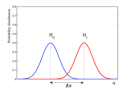
Figure 1: Distributions of likelihood ratio test statistic $q$ for the two hypotheses $H_{0}$ and $H_{1}$ and the definition of $Z$.

In frequentist terminology $Z$ is conventionally called the median or expected significance. The median value of $q$ under hypothesis $H_{1}$ is denoted by $q_{A}$. This corresponds to the value of the likelihood ratio statistic obtained with the so called “Asimov” data set, which for poisson or gaussian data is just the expected value of the data $x$ under hypothesis $H_{1}$. The observed significance, i.e. the distance between the observed $q$ and $H_{0}$ in units of standard deviation is given by

$$z^{obs}=\frac{q+q_{A}}{2\sqrt{q_{A}}}$$ (2)

and the corresponding $p$-value is $1-\Phi(z^{obs})$, where $\Phi$ is the standard normal cumulative distribution. The median significance which is obtained by $q=q_{A}$ is therefore

$$z^{med}=Z=\sqrt{q_{A}}.$$ (3)

Note that while $q$ does not have a $\chi^{2}$ distribution, the median significance is related to the median $q_{A}$ via the simple relation $Z=\sqrt{q_{A}}$.

The Bayesian posterior probability of $H_{1}$ (assuming equal prior probabilities for both hypotheses) is given directly from the likelihood ratio by

$$P(H_{1})=(1+e^{-q/2})^{-1}.$$ (4)

Since $z^{obs}$ is a standard normal random variable, any quantile of a monotonically related quantity such as $P(H_{1})$ can be immediately calculated by substituting the corresponding quantiles of $z^{obs}$. For example, the central 68% ‘sensitivity band’ is obtained by taking $z^{obs}=[Z+1,Z-1]$, that is

$$q_{\pm 1}=q_{A}\pm 2\sqrt{q_{A}}=Z^{2}\pm 2Z,$$ (5)

and by substituting this into (4) one gets the corresponding quantiles for $P(H_{1})$.

The average posterior probability is given by

$$E[P(H_{1})]=\int_{-\infty}^{+\infty}dqf(q|H_{1})(1+e^{-q/2})^{-1}$$ (6)

and by noting that $P(H_{1})$ is smaller than $1/2$ when $q<0$ the following simple bound can be derived:

$$E[P(H_{1})] \leq \mbox{\small$\frac{1}{2}$}\int_{-\infty}^{0}dqf(q|H_{1})+\int_{0}^{+\infty}dqf(q|H_{1})$$

$$= 1-\mbox{\small$\frac{1}{2}$}\Phi(-Z/2)$$

which implies that the averaging has a similar effect, roughly, to reducing $Z$ by half. In Fig. 2 we compare this bound on the average value of $P(H_{0})=1-P(H_{1})$ with several of its quantiles from Eq.(4), which illustrates how the expectation is pushed to the tail of the distribution as $q_{A}=Z^{2}$ increases. For $q_{A}=100$, $E[P(H_{0})]$ is above $10^{-7}$ (comparable to “$5\sigma$”), which is well above the 1 per mil upper quantile. The 1% quantile for $q_{A}=100$ is already much lower at $10^{-12}$, meaning that there is 99% probability that the experiment will produce a level of evidence at least as high. In other words, such an experiment is almost guaranteed to produce an outcome with a level of evidence that is vastly superior to its average value.

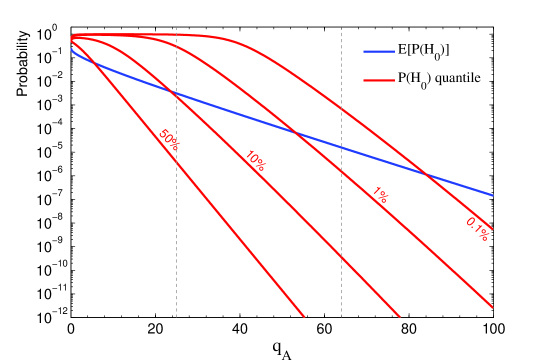
Figure 2: Blue curve: lower bound on the average value of the posterior probability $E[P(H_{0})]$ under hypothesis $H_{1}$. The actual average lies above the blue line. Red curve: several quantiles of the distribution of $P(H_{0})$ under hypothesis $H_{1}$. The two vertical dotted lines correspond to Z=5 and Z=8.

We finally note that a similar problem will arise if one would attempt to calculate the average $p$-value: this can be shown by direct calculation to be equal to $1-\Phi(Z/\sqrt{2})$, which again corresponds to a much lower significance level ($Z/\sqrt{2}$) than the median.

2.1 Another sensitivity measure

A different sensitivity measure introduced in Ref. [2] and applied e.g. in Ref. [9], was defined as “the probability of determining the correct hierarchy”, namely the probability that the likelihood ratio will favor the true hypothesis, i.e. $P(q>0)=1-\Phi(Z/2)$. This obviously also leads to a sensitivity measure that is equal to exactly half of the convention described above, although for a very different reason. We therefore stress the very different meanings of these two definitions:
Determination of the mass hierarchy with 5$\sigma$ confidence level (a “5$\sigma$ discovery”) formally implies that the probability of making an error, i.e. choosing the wrong hierarchy, is less than $3\times 10^{-7}$. Therefore:

• An experiment with $Z=5$ has a 50% probability of making a 5$\sigma$ discovery, and a typical observed significance will be in the range 4$\sigma$ – 6$\sigma$ (with 68% probability)

• An experiment with $Z=10$ has a 100% probability, i.e. is guaranteed to make a 5$\sigma$ discovery, and a typical observed significance will be in the range 9$\sigma$ – 11$\sigma$ (with 68% probability).

It should be clear that the definition of “5$\sigma$ sensitivity” adopted in [9] corresponds to the second case above, i.e. to Z=10.

3 Conclusions

The average posterior probability can severely under-estimate the actual sensitivity of an experiment, in terms of its probability to achieve high levels of evidence. This can be seen by comparing the average to the median and other quantiles that have a simple relation to the median likelihood ratio test statistic evaluated with the “Asimov” data set. Furthermore the sensitivity measure that is defined by the “probability of determining the correct hierarchy” leads to a similar effect. The meaning of such estimates should be well understood and not confused with the common convention.

References

- [1] K. Nakamura et al., Review of Particle Physics, J. Phys., G37:075021, 2010.
- [2] X. Qian et al., Statistical evaluation of experimental determinations of neutrino mass hierarchy, Phys. Rev. D, 86 11 (2012), [arXiv:1210.3651]
- [3] X. Qian et al., Mass hierarchy resolution in reactor anti-neutrino experiments: Parameter degeneracies and detector energy response, Phys. Rev. D 87, 033005 (2013).
- [4] A.B. Balantekin et al., Neutrino mass hierarchy determination and other physics potential of medium-baseline reactor neutrino oscillation experiments, [arXiv:1307.7419]
- [5] DELPHI Collaboration (P. Abreu et al.), Eur. Phys. J. C 17 (2000) 187-205.
- [6] A. L. Read, proceedings of the 1st Workshop on Confidence Limits, CERN, Geneva, Switzerland, 17 - 18 Jan 2000, pp.81-101, CERN-OPEN-2000-205.
- [7] For a recent example see e.g. figures 7,9 in Aad, G. et al., Phys.Lett. B716 (2012) 1-29 arXiv:1207.7214 [hep-ex] CERN-PH-EP-2012-218.
- [8] G. Cowan, K. Cranmer, E. Gross and O. Vitells, Asymptotic formulae for likelihood-based tests of new physics, Eur. Phys. J. C 71 (2011) 1544, [arXiv:1007.1727].
- [9] The LBNO Consortium, CERN-SPSC-2013-032, http://cds.cern.ch/record/1612207.