A thermostatistical approach to scale-free networks

Abstract

We describe an ensemble of growing scale-free networks in an equilibrium framework, providing insight into why the exponent of empirical scale-free networks in nature is typically robust. In an analogy to thermostatistics, to describe the canonical and microcanonical ensembles, we introduce a functional, whose maximum corresponds to a scale-free configuration. We then identify the equivalents to energy, Zeroth-law, entropy and heat capacity for scale-free networks. Discussing the merging of scale-free networks, we also establish an exact relation to predict their final “equilibrium” degree exponent. All analytic results are complemented with Monte Carlo simulations. Our approach illustrates the possibility to apply the tools of equilibrium statistical physics to study the properties of growing networks, and it also supports the recent arguments on the complementarity between equilibrium and nonequilibrium systems.

1 Introduction

The theory of thermal equilibrium is one of the most important milestones in the development of statistical and theoretical physics. Most mesoscopic processes are, however, far from equilibrium, and describe the flow of energy through a system. Often the cascaded transfer and eventual dissipation of this energy leads to the appearance of scale-free structures, characterized by power laws. Describing nonequilibrium systems in a equilibrium framework would give access to the vast array of tools developed for the equilibrium case. Such paralelism is not straightforward. Nevertheless, important equivalences between the two descriptions have recently been established [1, 2].

With the aim of strengthen further the bridge between equilibrium and non-equilibrium systems, we explore such apparent equivalences in the context of complex networks. Networks are general means to describe the topology of interactions, where nodes are the agents and the links represent the interactions. Scale-free networks (SFNs) are characterized by a power-law degree distribution and have been found in several socio-technical systems, such as airline networks, Internet, phone calls patterns, and reservoir networks [3, 4, 5, 6]. Insofar, SFNs have been described as products of growth processes as, e.g., preferential attachment [7, 8], and therefore classified as nonequilibrium networks [9].

In this Letter, we present a mapping of a specific ensemble of SFNs into an equilibrium ensemble by properly rescaling the growing values of the connection strength, and we apply the tools of thermostatistics to measure several network properties. We derive the equivalents to micro- and macrostates and show how properties such as energy and entropy can be defined. While the number of nodes is kept constant, the number of connections grows in time.

For the specific case that the weights correspond to the degrees $k$ of the nodes, we present a series of Monte-Carlo simulations, both in the canonical and the microcanonical formalism, illustrating that the scale-free networks follow the equivalent of a Zeroth law, i. e. (i) a network brought in contact with a reservoir relaxes to an “equilibrium” state with the same degree distribution as the reservoir, (ii) two “equilibrated” networks with different degree distributions brought in contact with each other develop a new “equilibrium” state with a new final degree distribution. We then show, (iii), that the final degree distribution can be calculated exactly from the equivalent of the heat capacity, which depends on the second moment of the energy.

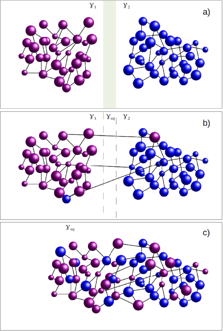
Figure 1: (Color online) When two scale-free networks of degree exponents $\gamma_{1}$ and $\gamma_{2}$ are put in contact, they evolve towards an “equilibrium” scale-free state of exponent $\gamma_{eq}$.

We start by defining a proper energy function that characterizes the microstates of a scale-free network. From this definition we then introduce the canonical and the microcanonical ensembles. From these ensembles we can then derive the explict expression for entropy and heat capacity as well as principles such as the Zeroth-law for scale-free networks. Discussion and conclusions end this paper.

2 The energy function for scale-free networks

The network here investigated consider an ensemble of $N$ nodes, where each node $i$ occupies one of $M$ possible microstates. Each microstate $j$ is characterized by a scalar $\hat{w}_{j}$, which we call connection strength or weight. This weight can be, for example, the degree of the node for undirected graphs, the in- or out-degree for directed ones, or the sum over the weight of the node links for a weighted graph. In every case, it is the weight that measures the local state of each node in the system, and therefore the energy function shall be a function of the weight alone.

Since weights grow in time, the state space is not constant, and thus one cannot denominate a statistical ensemble. To overcome that shortcoming we define a rescaled weight $w_{j}$ as,

$$w_{j}=\frac{\hat{w}_{j}-\hat{w}_{\textrm{min}}}{\hat{w}_{\textrm{max}}-\hat{w}_{\textrm{min}}}\ \ ,$$ (1)

where $\hat{w}_{\textrm{min}}$ and $\hat{w}_{\textrm{max}}$ are the minimum and maximum weights, such that $w_{j}$ is in the range $[0,1]$, for all states $j=1,\dots,M$. With this rescaling, we then have a time-independent probability space, over which we can derive a microcanonical evolution equation.

Assuming that the weights are an equivalent of an energy flow into the system, the next question is: Which functional dependence on the weight should the energy function have? Here we argue that the proper choice for the energy function of the microstate $j$ is

$$\epsilon_{j}=\log{w_{j}}.$$ (2)

Why is the logarithmic function of the weight the proper one for defining an energy interchange among nodes in a scale-free network? The answer might lie in the typical self-similarity of scale-free networks[4]. In time-evolving processes one usually looks for periodicities, i.e. invariants under a given time shift. For an ordered set of different scales the corresponding feature of periodicity is self-similarity[10]: a perfectly self-similar process variable $w$ is invariant when shifting from one scale to another, $\lambda$, i.e. the probability distribution function remains invariant $p(\lambda^{n}\omega)=\lambda p(\omega)$, as do its moments.

Through the rescaling of the weights in scale-free networks one is able to obtain a stationary probability space, in which the evolution of canonical and microcanonical ensembles can be formulated. For that, it is necessary to identify the logarithmic weight as the energy function of each microstate. In other words, while SFNs evolve with no conservation of their average degree, the total logarithmic weight is conserved, which should be taken therefore as the total energy.

3 Canonical scale-free networks

To derive the canonical ensemble of scale-free networks we first define each macrostate of the system. One macrostate $W$ is completely defined by the distribution of the $N$ nodes among the microstrates: $W\equiv W(n_{1},\dots,n_{M})$, where $n_{j}$ is the occupation number of state $j$. For each macrostate there are $\Omega=\frac{N!}{\prod_{j}n_{j}!}$ equivalent configurations or microstates. Using Boltzmann’s entropy, the entropy $S$ of a macrostate is $S=\log{\Omega}$.

Having two of such systems (networks), as sketched in Fig. 1, we now consider that they evolve in time, i.e. connections are created and destroyed in time according to some criteria, reflecting an interchange of energy among the nodes which, consequently hop between microstates. We next introduce the canonical ensemble, which describes the distribution among microstates for one single network, taking the other one in Fig. 1 as a heat reservoir. After that we discuss the microcanonical ensemble where both networks are of the same size.

Figure 2 illustrates the evolution of a canonical scale-free ensemble. We started with a regular random graph with $N=10^{5}$ nodes, each one having $k=5$ neighbors, and put it in contact with a large scale-free network (reservoir) with $N=10^{7}$ nodes and exponent $\gamma=3$. The latter was obtained using the described algorithm after a sufficiently large number of interactions. As one clearly sees throughout the four stages plotted in Fig. 2, the degree distribution evolves towards a power-law distribution with the same exponent. While in this implementation the number $L$ of links is kept constant, similar results are obtained for a network with $L$ growing in time; in that case, instead of degree, one considers the normalized degree similar to the weight in Eq. (1).

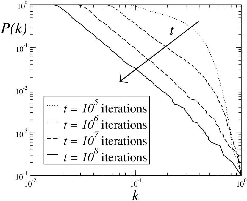
Figure 2: The scale-free canonical ensemble: starting with a uniform distribution of degree among $N=10^{5}$ nodes in contact with a reservoir ($N=10^{7}$ nodes) having a distribution $P(k)\sim k^{-\gamma}$ with $\gamma=3$ , the degree distribution of the system evolves towards the same power-law.

In a more general canonical framework, where one has a weight defined by Eq. (1), the most probable macrostate is the one that maximizes the entropy. This maximization has two constraints: conservation of the average total energy, which with the definition (2) reads $E=\sum_{j}n_{j}\log{w_{j}}$, and of the number of nodes, $N=\sum_{j}n_{j}$.

Together with the definition of entropy above, the most probable macrostate is an extremum of the functional,

$${\cal{F}}=\log{\Omega}-\gamma\sum_{j=1}^{M}n_{j}\log{w_{j}}+\log{\alpha}\sum_{j=1}^{M}n_{j},$$ (3)

where $\gamma$ and $\log{\alpha}$ are the Lagrange multipliers for the constraints in the energy and number of nodes, respectively. For thermodynamic ensembles, $\gamma$ is the inverse of the reservoir “temperature” and $\log{\alpha}$ the ratio between the “chemical potential” and the temperature. Interestingly, from this approach one concludes that $\gamma$ is a property of the reservoir, while $\log{\alpha}$ is characteristic of the system.

Using Stirling’s approximation one obtains that the extrema of Eq. (3) yield $n_{j}=\alpha w_{j}^{-\gamma}$. If we define $\hat{w}_{i}=k_{i}$, where $k_{i}$ is the node degree, the degree distribution is a power law of degree exponent $\gamma$. In other words, the reservoir sets the degree exponent. The weight distribution is consistent with the expected Boltzmann distribution for canonical ensembles. Note that the node energy is $\epsilon_{i}=\log{w_{i}}$, which is thereby exponentially distributed.

In fact, as claimed by other authors, if properly interpreted, the Boltzmann distribution yield “disguised” power laws [11, 12]. In our case, the power law reflects the degree distribution $P(k)\sim k^{-\gamma}$ of the connections among the nodes of the system in contact with a “heat” reservoir having a constant “temperature”, i.e. a very large network with a given exponent for its power-law degree distribution. Notice that, the subnetwork converge to a SFN by randomly interchanging connections with the reservoir: no preferential attachment is here required. One therefore obtains a SF topology from an arbitrary initial weight distribution and a succession of random exchanges of connections with a SF reservoir. See Fig. 2.

To generate such “equilibrium” networks with degree exponent $\gamma$, the canonical formalism was numerically implemented as follows. One starts with $N$ nodes, interconnected through $L$ links, yielding a certain degree distribution, $\{k_{i}\}$. At each iteration, one randomly selects two nodes, $l$ and $m$, and calculates the change $\Delta E$ in the total energy $E$ if one link connected to $l$ is rewired to be connect to $m$,

$$\Delta E=\Delta(\log{k_{l}})+\Delta(\log{k_{m}})\ \ .$$ (4)

This rewiring is executed with probability $p=\min\left\{1,\exp\left(-\gamma\Delta E\right)\right\}$. After some iterations, the network converges to the desired scale-free degree distribution. Since $\epsilon_{i}=\log{k_{i}}$, the energy is only conserved for movements where $k^{\mathrm{initial}}_{l}=k^{\mathrm{initial}}_{m}+1$, where $k^{\mathrm{initial}}_{l}$ and $k^{\mathrm{initial}}_{m}$ are the degree of nodes $l$ and $m$ before the movement. This algorithm is an instance of the Metropolis algorithm, thus respects detailed balance[13].

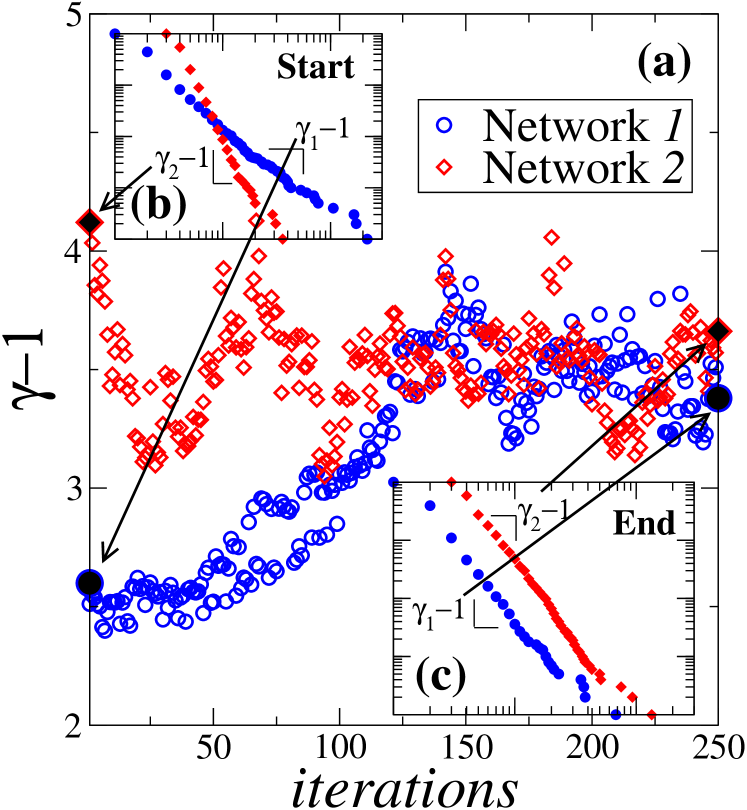
Figure 3: (Color online) (a) Evolution of the degree exponent of two scale-free networks in contact with each other. Initially, the two networks have different degree exponents (inset (b)) but converge towards a degree distribution with the same degree exponent $\gamma_{\mathrm{eq}}$ (inset (c)). All represented values refer to cumulative distributions.

4 Microcanonical scale-free networks

We consider now the classical problem of thermal equilibration. What is the final degree distribution when two scale-free networks are put in contact? To address this question, as schematically illustrated in Fig. 1, we consider two scale-free networks of degree exponent $\gamma_{1}$ and $\gamma_{2}$. Since the combined system is isolated, the total energy $E_{1+2}=E_{1}+E_{2}$ is expected to be conserved, where $E_{1}$ and $E_{2}$ is the energy of networks $1$ and $2$, respectively. Figure 3a shows the evolution of the degree exponent of the nodes in each network, using the microcanonical algorithm proposed below. The two networks merge into one with a power-law degree distribution of exponent $\gamma_{\mathrm{eq}}$.

This situation is described through a microcanonical ensemble, which represents an isolated network at a given energy. To numerically explore the configuration space we propose a generalization of the Creutz algorithm, which respects both detailed balance and ergodicity[14]. Let us consider again the case where the weight corresponds to the degree. Algorithmically, instead of interacting with a heat reservoir like in the canonical case, the network exchanges energy with one energy reservoir, named demon, with energy $E_{\mathrm{demon}}$. One starts with one network at the desired energy and $E_{\mathrm{demon}}=0$. As in the canonical simulation, at each iteration two nodes $l$ and $m$ are randomly selected and the energy change of the rewiring movement is obtained from Eq. (4). If $\Delta E\leq 0$, the movement is accepted and the energy difference is transferred to the demon. Otherwise, the movement is only accepted if $E_{\mathrm{demon}}>\Delta E$, and, when it happens, the energy difference is subtracted from $E_{\mathrm{demon}}$. To obtain a network with a pre-given energy $E$, one can also start with the subnetwork having the desired number of links and nodes and energy $E_{1+2}<E$ and impose $E_{\textrm{demon}}=E-E_{0}$. After a few iterations the network energy converges towards $E$.

To illustrate the microcanonical ensemble of scale-free networks we implemented the algorithm above for two subnetworks, each one composed of $N=10^{5}$ nodes and a power-law degree distribution, but having different exponents, namely $\gamma_{1}\approx 7/2$ and $\gamma_{2}\approx 5$. Figure 3b shows the initial degree distribution of each subnetwork. As shown in Figs. 3b and 3c, the degree distribution of the set of nodes initially belonging to subnetworks 1 and 2 converges towards the same degree exponent, $\gamma_{eq}\approx 9/2$.

5 Thermostatistics of scale-free networks

With the thermostatistic approach proposed here, one can derive five results for ensembles of scale-free networks. First, the equivalent to the Zeroth-law of thermodynamics can be expressed as: if networks $A$ and $B$ are in equilibrium with network $C$ then they are also in equilibrium with each other. Here, two networks in equilibrium have the same degree exponent $\gamma$.

Second, one can derive a closed expression for the entropy of scale-free networks. As discussed before, each macrostate has $\Omega$ possible equivalent configurations. Substituting the power-law solution in Eq. (3) in the definition of $\Omega$, yields for the entropy

$$S=\log{\Omega}=S_{0}+\gamma\alpha\sum_{i=1}^{M}{w_{i}^{-\gamma}\log{w_{i}}}\ \ ,$$ (5)

where $S_{0}=N\log{\left(\sum_{i=1}^{N}w_{i}^{-\gamma}\right)}$ is the minimum entropy and the second term is equivalent to the Shannon entropy. This expression for the entropy complements previous works[15].

Third, in the continuum limit, associated with a large number of microstates $M$, the sum in Eq. (5) can be approximated by an integral, yielding an expression for $S$, solely depending on $\gamma$ and $N$. The differential of the entropy is then,

$$dS=\frac{\partial S}{\partial\gamma}d\gamma+\frac{\partial S}{\partial N}dN\ \ .$$ (6)

Equation (6) tell us that the network entropy can either change due to removal or addition of nodes ($dN\neq 0$), similar to the procedures introduced by Barabasi, Newman and others[4] or due to rewiring[16], “energy” exchange ($d\gamma\neq 0$), as reported here.

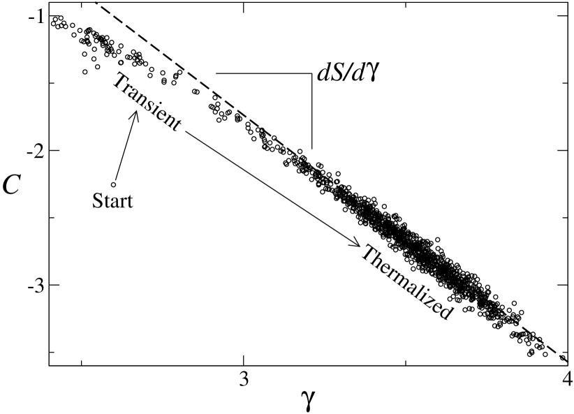
Figure 4: The heat capacity $c_{N}$ versus exponent $\gamma$ for the microcanonical ensemble of two scale-free networks. The negative-valued slope of the linear dependence between $c$ and $\gamma$ gives the constant value $\frac{dS}{d\gamma}$. See Fig. 5.

Fourth, we can define a heat capacity for non-growing scale-free networks, which can be obtained from the entropy as,

$$c_{N}=\gamma\left(\frac{dS}{d\gamma}\right)_{N}=\gamma\langle\log{w}\rangle-\gamma^{2}\langle(\log{w})^{2}\rangle\ \ .$$ (7)

Figure 4 shows the pair $(c_{N},\gamma)$ of the system of interacting networks addressed in Fig. 3. One clearly sees a linear dependence with a negative slope, $(\frac{dS}{d\gamma})_{N}<0$, which can be understood since $\gamma$ plays the role of the inverse of a temperature.

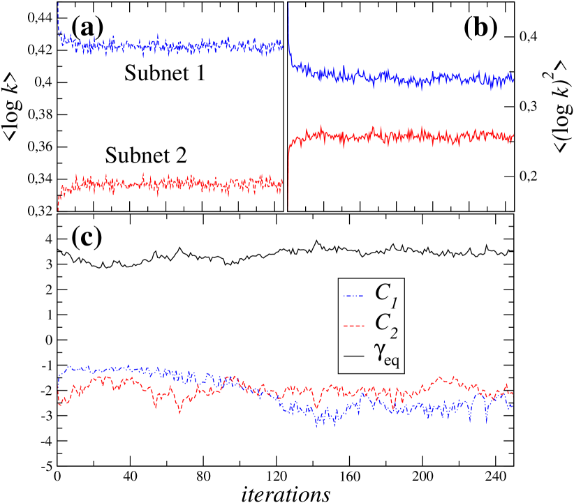
Figure 5: (Color online) Computing equilibrium exponents and heat capacity of scale-free networks: (a) first and (b) second moments of the energy $e_{i}\equiv\log{w_{i}}=\log{k_{i}}$ in two separated unweighted scale-free networks (blue and red). (c) The corresponding heat capacities, $c_{1}$ and $c_{2}$ (Eq. (7)) and equilibrium exponent $\gamma_{eq}$ (Eq. (9)).

Fifth, one can predict the value of the exponent $\gamma_{\mathrm{eq}}$ when two networks of different degree exponents, $\gamma_{1}$ and $\gamma_{2}$, interact. Due to the interaction, internal links of each network are rewired to connect to the other network. The variation of energy $E_{l}$, which accounts for the overall variation of logarithmic of the number of connections in network $l={1,2}$ obeys the relation,

$$\Delta E_{l}=c_{l}\left(\gamma_{\mathrm{eq}}-\gamma_{l}\right)\ \ ,$$ (8)

where $c^{(l)}$ is the heat capacity of network $l$. As the number of links is conserved, $\Delta E_{1}=-\Delta E_{2}$. Consequently,

$$\gamma_{\mathrm{eq}}=\frac{c_{1}\gamma_{1}+c_{2}\gamma_{2}}{c_{1}+c_{2}}\ \ .$$ (9)

Indeed, Eq. (9), together with Eq. (7), provide a simple way for predicting the equilibrium exponent of two scale-free networks that merge.

Figure 5a and 5b shows respectively the evolution of the quantities $\langle\log{\gamma}\rangle$ and $\langle(\log{\gamma})^{2}\rangle$ in Eq. (7) for computing the heat capacity, $c_{1}$ and $c_{2}$ in each network, which we plot in Fig. 5c together with $\gamma_{eq}$ calculated from Eq. (9). The result for $\gamma_{eq}$ are consistent with the ones plotted in Fig. 3.

6 Discussion and conclusions

In summary, we presented an equilibrium description of scale-free networks with a growing number of connections. A thermostatistical framework was established, defining canonical and microcanonical ensembles of power-law distributions. With an algorithm for microcanonical ensembles, we showed that the merging of two scale-free networks, with different exponents, evolves towards an equilibrium power-law distribution. Moreover, we show how to predict the equilibrium exponent when two scale-free networks merge.

We have replaced, through rescaling, the growing system (growing $k$), which has an influx of energy (increasing $\epsilon_{j}$) by a corresponding “isolated” system which obeys thermostatistical laws. As should be noted, a similar choice for the energy has been made in the context of Bose-Einstein condensation in networks[17].

Future work might focus on the geometrical properties of this new ensemble of networks. We consider a statistical ensemble of networks, with a time-dependent weight for each node, which is used to define an equivalent to the energy of one microstate. We then prescribe an iterative re-weighting procedure, such that a functional, which contains the analogue of the entropy, is maximized, while constraining the average total energy and number of nodes. We present expressions for the thermostatistical variables. From this, we propose the existence of canonical and microcanonical ensembles, which are scale-free networks with maximum entropy. We employ rescaling of the number of links, which is not necessarily time invariant, and we focus on networks with a constant number of nodes[18].

This new framework might provide insight into other problems. For example, recently an interesting study of the Romenian wealth distribution revealed that the evolution of the wealth distribution yields a power law robust against external forcing and perturbations (changes in policy, tax laws, …) [19]. The size of the Romanian society is considered to be approximately constant in time, but the links (economical interactions) are dynamic. In the spirit of the framework we describe here, one might speculate that the robustness of the power-law distribution is characteristic of an “equilibrium” state as the one reported here. Well known examples of robust power-law distributions, with approximately constant exponent in time, are also the Internet and the WWW. In this case, the number of nodes is dynamic. A generalization of our framework to networks with varying number of nodes might also help understanding such robustness.

- [1] \NameChetrite R. Touchette H. \REVIEWPhys. Rev. Lett. 1112013120601.
- [2] \NameJavarone M. Armano G. \REVIEWJ. Stat.Mech. 042013P04019.
- [3] \NameGuimera R., Mossa S., Turtschi A. Amaral L. A. N. \REVIEWProc. Nat. Acad. Sci. USA 10220057794.
- [4] \NameAlbert R. Barabási A.-L. \REVIEWReview of Modern Physics 74200247.
- [5] \NameGonzalez M., Hidalgo C. Barabasi A. \REVIEWNature 4532008779.
- [6] \NameMamede G., Araújo N., Schneider C., de Araújo J. Herrmann H. \REVIEWProc. Nat. Acad. Sci. USA 10920127191.
- [7] \NameBoccaletti S., Latora V., Moreno Y., Chavez M. Hwang D.-U. \REVIEWPhysics Reports 4242006175.
- [8] \NameCastellano C., Fortunato S. Loreto V. \REVIEWReviews of Modern Physics 812009591.
- [9] \NameDorogovtsev S., Goltsev A. Mendes J. \REVIEWReviews of Modern Physics 8020081275.
- [10] \NameSchroeder M. \BookFractals, Chaos, Power-laws (W.H. Freeman and Co.) 1991.
- [11] \NameLevy M. Solomon S. \REVIEWInternational Journal of Modern Physics C 71996595.
- [12] \NameRichmond P. Solomon S. \REVIEWInt. J. Mod. Physics 122001333.
- [13] \NameMetropolis N., Rosenbluth A., Rosenbluth M., Teller A. Teller E. \REVIEWJ. Chem. Phys. 2119531087.
- [14] \NameCreutz M. \REVIEWPhys. Rev. Lett. 5019831411.
- [15] \NamePark J. Newman M. \REVIEWPhysical Review E 702004066117.
- [16] \NameSchneider C. M., Moreira A. A., Andrade Jr. J. S., Havlin S. Herrmann H. J. \REVIEWProc. Nat. Acad. Sci. USA 10820113838.
- [17] \NameBianconi G. Barabási A.-L. \REVIEWPhys. Rev. Lett. 8620015632.
- [18] \Nameda Cruz J. \BookCriticality in economy Phd thesis University of Lisbon (2014).
- [19] \NameDerzsy N., Neda Z. Santos M. \REVIEWPhysica A 39120125611.