Neighborhood filters and the decreasing rearrangement

Abstract

Nonlocal filters are simple and powerful techniques for image denoising. In this paper, we give new insights into the analysis of one kind of them, the Neighborhood filter, by using a classical although not commonly used transformation: the decreasing rearrangement of a function. Independently of the dimension of the image, we reformulate the Neighborhood filter and its iterative variants as an integral operator defined in a one-dimensional space. The simplicity of this formulation allows to perform a detailed analysis of its properties. Among others, we prove that the filtered image is a contrast change of the original image, an that the filtering procedure behaves asymptotically as a shock filter combined with a border diffusive term, responsible for the staircaising effect and the loss of contrast.

keywords: Neighborhood filters, decreasing rearrangement, denoising, segmentation

1 Introduction

Let $\Omega\subset\mathbb{R}^{d}$ $(d\geq 1)$ be an open and bounded set, and consider a function $u\in L^{\infty}(\Omega)$. The Neighborhood filter operator is defined by

$$\operatorname{NF}^{h}u(\mathbf{x})=\frac{1}{C(\mathbf{x})}\int_{\Omega}\textrm{e}^{-\frac{|u(\mathbf{x})-u(\mathbf{y})|^{2}}{h^{2}}}u(\mathbf{y})d\mathbf{y},$$ (1)

where $h$ is a positive constant, and

$$C(\mathbf{x})=\int_{\Omega}\exp\left(-|u(\mathbf{x})-u(\mathbf{y})|^{2})h^{-2}\right)d\mathbf{y}$$

is a normalization factor, intended to allow constants to be fixed points of $\operatorname{NF}^{h}$.

The Neighborhood filter (NF) is the simplest particular case of other related filters involving local terms, notably the Yaroslavsky filter [31, 32], the SUSAN filter [27] introduced by Smith and Brady, the Bilateral filter [30] of Tomasi and Manduchi, and the Nonlocal Means filter (NLM) [6] by Buades, Coll and Morel.

These methods have been introduced in the last decades as efficient alternatives to local methods such as those expressed in terms of nonlinear diffusion partial differential equations (PDE’s), among which the pioneering approaches of Perona and Malik [21], Álvarez, Lions and Morel [2] and Rudin, Osher and Fatemi [25] are fundamental. We refer the reader to [9] for a review and comparison of these methods.

Among all these filters, the Neighborhood filter is the simplest, but yet useful, method due to its compromise between denoising quality and computational speed. Indeed, although it creates shocks and staircasing effects [8], the computational cost is by far lower than those of other integral kernel filters or PDE’s based methods.

Since, usually, a single denoising step of the nonlocal filters is not enough, an iteration is performed according to several choices of the iteration actualization, see (3) and (4) for two of such strategies.

In this context, the Neighborhood filter and its variants have been analyzed from different points of view. For instance, Barash [3], Elad [13], Barash et al. [4], and Buades et al. [7] investigate the asymptotic relationship between the Yaroslavsky filter and the Perona-Malik PDE. Gilboa et al. [16] study certain applications of nonlocal operators to image processing. In [22], Peyré establishes a relationship between the non-iterative nonlocal filtering schemes and thresholding in adapted orthogonal basis. In a more recent paper, Singer et al. [26] interpret the Neighborhood filter as a stochastic diffusion process, explaining in this way the attenuation of high frequencies in the processed images.

In this article, we reformulate the Neighborhood filter in terms of the decreasing rearrangement of the initial image, $u$, which is defined as the inverse of the distribution function $q\in\mathbb{R}\to m_{u}(q)=|\{\mathbf{x}\in\Omega:u(\mathbf{x})>q\}|$, see Section 2 for the precise definition.

Realizing that the structure of level sets of $u$ is invariant through the Neighborhood filter operation as well as through the decreasing rearrangement of $u$ allows us to rewrite (1) in terms of a one-dimensional integral expression, see Theorem 1.

Although from expression (1) is readily seen that only computation on level lines is needed to perform the filtering, the alternative expression in terms of the decreasing rearrangement offers room for further analysis of the iterative scheme.

Perhaps, the most important consequence of the rearrangement is, apart from the dimensional reduction, the reinterpretation of the NF as a local algorithm. Thanks to this, we may prove some properties of the Neighborhood filter nonlinear iterative scheme, see (4), among which

• The asymptotic behavior of the NF as a shock filter of the type introduced by Álvarez et al. [1], combined with a contrast loss effect, see Theorem 3.

• The contrast change character of the NF, i.e. the existence of a continuous and increasing function $g:\mathbb{R}\to\mathbb{R}$ such that $\operatorname{NF}^{h}(u(\mathbf{x}))=g(u(\mathbf{x}))$, see Corollary 2.

As mentioned above, the most salient advantage of the Neighborhood filter in its rearranged version is speed. If $N$ denotes the image size in pixels, the complexity of other nonlocal filters such as the classical NF, the Bilateral or the NLM filters are of the order $C\times N$, where $C$ depends on different parameters (window sizes) used in those models. A typical value of $C$ may be of the order $10^{5}$, for the NLM. However, the complexity of the rearranged version of the NF depends on the number of the initial image intensity levels, which we assume quantized in $Q$ levels, and on some small constant related to the window size, $h$, resulting in a complexity of the order $c\times Q$, being a typical value of $c$ of the order $10^{2}$. Thus, the complexity of the NF is independent of the image size, once the level lines of the initial image have been identified.

However, denoising quality of the NF is, by far, poorer. The staircaising effect, always present in algorithms reducing the Total Variation of the initial image, is especially strong for the NF. In fact, after several iterations, and depending on the window size $h$, the NF output image concentrates most of its pixels mass on few level sets, producing a segmentation-like effect on the initial image.

A quick explanation of the difference between the NF and the Bilateral and NLM filters is that the NF does not retain any local information of the image, diffusing the intensity values just according to the mass of their corresponding level lines. Thus, a pixel belonging to a level line with large mass will retain its value even if it is isolated in a component of the image with different intensity value.

Due to this, the Neighborhood filter and morphological filters deduced from the topographic map of an image, see for instance the monograph by Caselles and Monasse [10], such as the Grain and the Killer filters, are also different since the latter use the local geometry of level sets connected components in a fundamental manner.

However, they do share some similitudes in their level set based framework, and this could be used for combining both algorithms. For instance, the isolated small regions belonging to a level line with large mass which remain in the filtered image after the NF application could be removed by morphological procedures, such as opening and closing operators.

The segmentation-like behavior of the NF may be explained in terms of the relationship between the inflexion points of the decreasing rearrangement and the local extreme points of the image histogram, $h(q)=-m^{\prime}_{u}(q)$. Thus, since the NF behaves asymptotically as a shock filter, and shock filters accumulate mass in inflexion points, we deduce that the NF works as an histogram based segmentation algorithm.

Since for our analysis the Gaussian form of the integral kernel is not important, we consider the following generalization of the Neighborhood filter

$$\operatorname{NF}^{h}u(\mathbf{x})=\frac{1}{C(\mathbf{x})}\int_{\Omega}\mathcal{K}_{h}(u(\mathbf{x})-u(\mathbf{y}))u(\mathbf{y})d\mathbf{y},$$ (2)

with $C(\mathbf{x})=\int_{\Omega}\mathcal{K}_{h}(u(\mathbf{x})-u(\mathbf{y}))d\mathbf{y}$, and $\mathcal{K}_{h}(\xi)=\mathcal{K}(\xi/h)$. For the moment, we only assume $\mathcal{K}\in L^{1}_{loc}(\mathbb{R})$ and $\mathcal{K}\geq 0$ to have (2) well defined, although more meaningful conditions will be stated later.

We consider the following iterative schemes, for $n\in\mathbb{N}$ (including $n=0$), and $u^{(0)}=u$:

1. Iteration with fixed kernel (linear operator),

   $$u^{(n+1)}(\mathbf{x})=\frac{1}{C_{0}(\mathbf{x})}\int_{\Omega}\mathcal{K}_{h}(u^{(0)}(\mathbf{x})-u^{(0)}(\mathbf{y}))u^{(n)}(\mathbf{y})d\mathbf{y},$$ (3)

   with $C_{0}(\mathbf{x})=\int_{\Omega}\mathcal{K}_{h}(u^{(0)}(\mathbf{x})-u^{(0)}(\mathbf{y}))d\mathbf{y}$.

2. Iteration with varying kernel (nonlinear operator),

   $$u^{(n+1)}(\mathbf{x})=\frac{1}{C_{n}(\mathbf{x})}\int_{\Omega}\mathcal{K}_{h}(u^{(n)}(\mathbf{x})-u^{(n)}(\mathbf{y}))u^{(n)}(\mathbf{y})d\mathbf{y},$$ (4)

   with $C_{n}(\mathbf{x})=\int_{\Omega}\mathcal{K}_{h}(u^{(n)}(\mathbf{x})-u^{(n)}(\mathbf{y}))d\mathbf{y}$.

Observe that, for both schemes, we have

$$\|u^{(n+1)}\|_{L^{\infty}(\Omega)}\leq\|u^{(n)}\|_{L^{\infty}(\Omega)},$$ (5)

for all $n\in\mathbb{N}$, and therefore the iterations are well defined.

The plan of the article is the following. In Section 2 we introduce the notion of decreasing rearrangement and establish the equivalence between (3) and (4) and its corresponding versions under this transformation. In addition, we show some examples on the relationship between an image and its relative rearrangement and histogram. In Section 3, we prove some qualitative properties of the nonlinear iterative scheme, among which its behavior as a shock filter. In Section 4, we describe the discretization of the continuous model and demonstrate with examples the denoising capabilities of the NF in comparison with the Bilateral and NLM filters, and its interpretation as a segmentation-like algorithm. In Section 5 we give our conclusions.

Finally, let us emphasize that the reformulation of the Neighborhood filter we propose produces the same filtered image than that obtained through the classical NF. However, there are two important advantages in our approach: (i) the filtering process is performed through a one-dimensional integral, reducing largely the algorithm complexity, and (ii) the rearranged version exposes the NF functioning to a deeper mathematical analysis.

2 Neighborhood filters in terms of the decreasing rearrangement

Let us denote by $|E|$ the Lebesgue measure of any measurable set $E$.

For a Lebesgue measurable function $u:\Omega\to\mathbb{R}$, the function $q\in\mathbb{R}\to m_{u}(q)=|\{\mathbf{x}\in\Omega:u(\mathbf{x})>q\}|$ is called the distribution function corresponding to $u$.

Function $m_{u}$ is non-increasing and therefore admits a unique generalized inverse, called the decreasing rearrangement. This inverse takes the usual pointwise meaning when the function $u$ has not flat regions, i.e. when $|\{\mathbf{x}\in\Omega:u(\mathbf{x})=q\}|=0$ for any $q\in\mathbb{R}$. In general, the decreasing rearrangement $u_{*}:[0,|\Omega|]\to\mathbb{R}$ is given by:

$$u_{*}(s)=\left\{\begin{array}[]{ll}{\rm ess}\sup\{u(\mathbf{x}):\mathbf{x}\in\Omega\}&\quad\text{if }s=0,\\ \inf\{q\in\mathbb{R}:m_{u}(q)\leq s\}&\quad\text{if }s\in(0,|\Omega|),\\ {\rm ess}\inf\{u(\mathbf{x}):\mathbf{x}\in\Omega\}&\quad\text{if }s=|\Omega|.\end{array}\right.$$

Notice that since $u_{*}$ is non-increasing in $[0,|\Omega|]$, it is continuous but at most a countable subset of $[0,|\Omega|]$. In particular, it is right-continuous for all $t\in(0,|\Omega|]$.

The notion of rearrangement of a function is classical. We refer the reader to the textbook [19] for the basic definitions and to the monograph [24] for a deeper insight into the subject.

The following equi-measurability property holds [24, Corollary 1.1.1]. Let $F:\mathbb{R}\to\mathbb{R}_{+}$ be a Borel function. Then

$$\int_{\Omega}F(u(\mathbf{y}))d\mathbf{y}=\int_{0}^{|\Omega|}F(u_{*}(s))ds.$$ (6)

In particular, $\|u\|_{L^{p}(\Omega)}=\|u_{*}\|_{L^{p}(0,|\Omega|)}$ for all $p\in[0,\infty]$.

We shall use the following notation for the level sets of $u$:

$$L_{t}(u)=\{\mathbf{y}\in\Omega:u(\mathbf{y})=u_{*}(t)\},\quad\text{for }t\in[0,|\Omega|].$$ (7)

The following theorem asserts that we may compute the Neighborhood filters in the one-dimensional space $[0,|\Omega|]$.

Theorem 1

Let $\Omega\subset\mathbb{R}^{d}$ be an open and bounded set, $d\geq 1$, and $\mathcal{K}:\mathbb{R}\to\mathbb{R}_{+}$ be a Borel function. Let $u^{(0)}\in L^{\infty}(\Omega)$ be, without loss of generality, non-negative and set $v_{0}=u^{(0)}_{*}$.

Then, for $m=0$ (resp. $m=n$), the iterative scheme (3) (resp (4)) may be computed as, for $\mathbf{x}\in L_{t}(u^{(0)})$ and $t\in[0,|\Omega|]$, $u^{(n+1)}(\mathbf{x})=v_{n+1}(t)$, with

$$v_{n+1}(t)=\frac{1}{c_{m}(t)}\int_{0}^{|\Omega|}\mathcal{K}_{h}(v_{m}(t)-v_{m}(s))v_{n}(s)ds,$$ (8)

and $c_{m}(t)=\int_{0}^{|\Omega|}\mathcal{K}_{h}(v_{m}(t)-v_{m}(s))ds$. In addition, for $n\in\mathbb{N}$,

$$\|v_{n+1}\|_{L^{\infty}(0,|\Omega|)}\leq\|v_{n}\|_{L^{\infty}(0,|\Omega|)}.$$ (9)

Proof. We start considering the one-step Neighborhood filter defined in (1). For each $\mathbf{x}\in\Omega$ such that $u(\mathbf{x})<\infty$ (i.e. all $\mathbf{x}\in\Omega$ but a subset of zero measure), we consider the Borel function $F:\mathbb{R}\to\mathbb{R}_{+}$ given by

$$F(w)=\mathcal{K}_{h}(u(\mathbf{x})-w)w\quad\text{if }w\geq 0,\quad F(w)=0\quad\text{if }w<0.$$ (10)

Then, (6) implies

$$\int_{\Omega}\mathcal{K}_{h}(u(\mathbf{x})-u(\mathbf{y}))u(\mathbf{y})d\mathbf{y}=\int_{0}^{|\Omega|}\mathcal{K}_{h}(u(\mathbf{x})-u_{*}(s))u_{*}(s))ds,$$

and

$$C(\mathbf{x})=\int_{0}^{|\Omega|}\mathcal{K}_{h}(u(\mathbf{x})-u_{*}(s))ds.$$

Since $\mathbf{x}\in L_{t}(u^{(0)})$, for some $t\in[0,|\Omega|]$, we have

$$\int_{0}^{|\Omega|}\mathcal{K}_{h}(u(\mathbf{x})- u_{*}(s))u_{*}(s))ds=\int_{0}^{|\Omega|}\mathcal{K}_{h}(u_{*}(t)-u_{*}(s))u_{*}(s))ds,$$

and similarly for $C(\mathbf{x})$.

We thus introduce the equivalent formulation to (1) given by, for $t\in[0,|\Omega|]$

$$\operatorname{NF}^{h}u(\mathbf{x})=\operatorname{NF}^{h}u_{*}(t)\quad\text{if}\quad\mathbf{x}\in L_{t}(u),$$ (11)

with

$$\operatorname{NF}^{h}u_{*}(t)=\frac{1}{c(t)}\int_{0}^{|\Omega|}\mathcal{K}_{h}(u_{*}(t)-u_{*}(s))u_{*}(s)ds,$$

and $c(t)=\int_{0}^{|\Omega|}\mathcal{K}_{h}(u_{*}(t)-u_{*}(s))ds$.

The extension of this transformation to the iterative schemes (3) and (4) ($m=0$ or $m=n$, respectively) is straightforward due to the invariance of the level sets structure with respect to the Neighborhood filtering, see (11). For both schemes, the step $n=1$ gives

$$u^{(1)}(\mathbf{x})=v_{1}(t):=\operatorname{NF}^{h}u_{*}^{(0)}(t),$$

for $\mathbf{x}\in L_{t}(u^{(0)})$. In the case of the scheme with variable kernel (4), we may use the same function $F$ defined in (10) to deduce that $u^{(2)}$ is constant in $L_{t}(u^{(0)})$ for each $t\in[0,|\Omega|]$. An induction argument allows us to define

$$u^{(n+1)}(\mathbf{x})=v_{n+1}(t):=\operatorname{NF}^{h}v_{n}(t),$$

for $n\in\mathbb{N}$, and $\mathbf{x}\in L_{t}(u^{(0)})$, which is (8) with $m=n$.

For the fixed kernel scheme (3) ($m=0$) we can not use $F$ in the step $n=1$ because the values of $u^{(0)}$ and $u^{(1)}$ inside the integral may be different on the level set $L_{t}(u^{(0)})$. However, these functions are still constant in each level set, implying the existence of a measurable function $f_{1}$ such that $f_{1}(u^{(1)}(\mathbf{x}))=u^{(0)}(\mathbf{x})$ for $\mathbf{x}\in L_{t}(u^{(0)})$, for $t\in[0,|\Omega|]$. Therefore, we may repeat the above argument with function $F$ replaced by $F_{1}(w)=\mathcal{K}_{h}(u^{(0)}(\mathbf{x})-f_{1}(w))w$ if $w\geq 0$ and $F_{1}(w)=0$ if $w<0$, thus obtaining

$$u^{(2)}(\mathbf{x})= \operatorname{NF}^{h}u^{(1)}(\mathbf{x})=\frac{1}{C_{1}(\mathbf{x})}\int_{0}^{|\Omega|}\mathcal{K}_{h}(u^{(0)}(\mathbf{x})-f_{1}(v_{1}(s))v_{1}(s)ds$$

$$= \frac{1}{C_{1}(\mathbf{x})}\int_{0}^{|\Omega|}\mathcal{K}_{h}(u^{(0)}(\mathbf{x})-u^{(0)}_{*}(s))v_{1}(s)ds.$$

Reasoning in a similar way for $C_{1}(\mathbf{x})$, and recalling the definition of $v_{0}$ we obtain for $\mathbf{x}\in L_{t}(u^{(0)})$,

$$u^{(2)}(\mathbf{x})=v_{2}(t):=\frac{1}{c_{1}(t)}\int_{0}^{|\Omega|}\mathcal{K}_{h}(v_{0}(t)-v_{0}(s))v_{1}(s)ds.$$

Then (8) for $m=0$. follows from an inductive argument.

Finally, using (5) and the equi-measurability property (6) we obtain (9) for all $n\in\mathbb{N}$. $\Box$

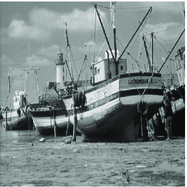
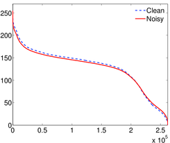
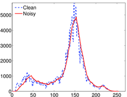
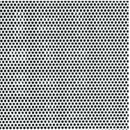
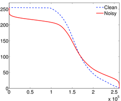
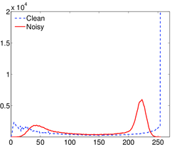
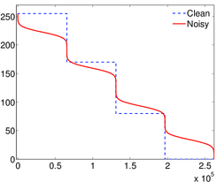
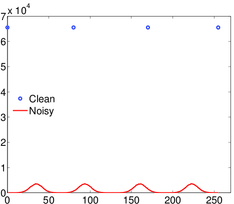
Figure 1: Test images Boat, Texture and Squares. Second and third columns show the decreasing rearrangement and the histogram, respectively, of the original images (clean) and their counterparts obtained after the addition of a Gaussian noise with SNR$=10$.

2.1 Examples

We show three examples of the decreasing rearrangement for clean and noisy images, all of them quantized in the usual interval $[0,255]$.

We have chosen as test images a natural image, Boat, a texture image, Texture, and a synthetic image, Squares. The first two images are taken from the data base of the Signal and Image Processing Institute, University of Southern California (boat.512.tiff of Vol. 3 and 1.5.02.tiff of Vol. 1, respectively), see [12, 18], while the third is a synthetic image constructed with four gray levels ($0,~{}85,~{}170$ and $255$) and such that its four level sets have the same measure.

This choice is motivated by the bad (resp. good) performance of the NF for uniform (resp. extreme) distribution of gray levels mass. These distributions are plotted in Fig. 1.

A gray levels mass uniformly distributed image has a straight line as decreasing rearrangement, or a constant, as histogram. In Fig. 1, we observe that the decreasing rearrangement of the Boat, is closer to a straight line than that of the Texture, which is still continuous. The choice of the synthetic image is motivated by its extreme behavior: a piece-wise constant decreasing rearrangement.

We have added a Gaussian white noise of $\text{SNR}=10$ to the test images according to the noise measure $\text{SNR}=\sigma(u)/\sigma(\nu)$, where $\sigma$ is the empirical standard deviation, $u$ is the original image, and $\nu$ is the noise.

We may observe in Fig. 1 that the main consequence of noise addition on the decreasing rearrangement is its smoothening towards a straight line. Of course, the effect is stronger in far from uniformly distributed images, like the Squares.

Finally, observe the connection between points of local maximum or minimum for the histogram and inflexion points for the decreasing rearrangement. This is the base for justifying the use of the NF as a segmentation algorithm.

3 Properties of the nonlinear varying-kernel iterative scheme

For the differential analysis we carry out in this section we have to assume regularity properties on the decreasing rearrangement of the given image.

In general, if $u\in W^{1,q}(\Omega)$, with $q>d$, and $\Omega$ is open, bounded and connected, then $u_{*}\in W^{1,p}(0,|\Omega|)$ for any $p<2$, see [24, Th. 3.3.2]. However, not much more than this is expected, and even for $C^{\infty}(\Omega)$ functions, their decreasing rearrangement may be non globally differentiable, see Fig. 2.

The following theorem asserts that the monotonicity property of the decreasing rearrangement of the initial image is conserved along all the iterations. In addition, for some type of kernels among which the Gaussian is included, the measure of flat regions does not change in the iterative procedure. We also obtain a condition in terms of the window size, $h$, ensuring that the steady state is a constant.

Theorem 2

Let $v_{0}=u^{(0)}_{*}\in W^{1,p}(0,|\Omega|)$ for some $p\geq 1$. Let $\mathcal{K}\in W^{1,\infty}_{\text{loc}}(\mathbb{R})$, with $\mathcal{K}(\xi)\geq 0$ for all $\xi\in\mathbb{R}$, and $\mathcal{K}(\xi)>0$ for all $\xi$ in a neighborhood of $0$.

Let $v_{n+1}$ be given by the iterative scheme (8), for $n\in\mathbb{N}$ and $m=n$. Then we have, for all $n\in\mathbb{N}$,

1. $v_{n+1}\in W^{1,p}(0,|\Omega|)$, and if $v^{\prime}_{0}(t)=0$ then $v^{\prime}_{n+1}(t)=0$.

2. Let $R_{1}:=(\xi_{1}-\xi_{2})\big{(}\mathcal{K}^{\prime}(\xi-\xi_{1})\mathcal{K}(\xi-\xi_{2})-\mathcal{K}^{\prime}(\xi-\xi_{2})\mathcal{K}(\xi-\xi_{1})\big{)}$ and assume

   $$R_{1}\geq 0\text{ for all }\xi,\xi_{1},\xi_{2}\in\mathbb{R}.$$ (12)

   Then $v^{\prime}_{n+1}\leq 0$ a.e. in $(0,|\Omega|)$. In addition, if $v^{\prime}_{0}(t)<0$ and the inequality in (12) is strict then $v^{\prime}_{n+1}(t)<0$.

3. Let $\phi:\mathbb{R}_{+}\to\mathbb{R}_{+}$ be a continuous function of $h$ such that $\lim_{h\to\infty}\phi(h)=0$. Assume that $\mathcal{K}>0$ in $\mathbb{R}$, and let

   $$R_{2}=(\xi_{1}-\xi_{2})\Big{(}\frac{\mathcal{K}^{\prime}(\xi-\xi_{1})}{\mathcal{K}(\xi-\xi_{1})}-\frac{\mathcal{K}^{\prime}(\xi-\xi_{2})}{\mathcal{K}(\xi-\xi_{2})}\Big{)}.$$

   Assume

   $$R_{2}\leq\phi(h)(\xi_{1}-\xi_{2})^{q}\quad\forall h\geq 0,\quad\forall\xi,\xi_{1},\xi_{2}\in\mathbb{R},$$ (13)

   for some $q\geq 1$. Then, if $h$ is large enough the sequence $v_{n}$ converges uniformly to a constant.

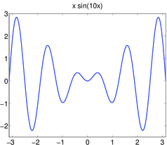
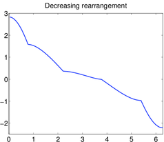
Figure 2: Graphic of function $f(x)=x\sin(10x)$ (top panel) and that of its decreasing rearrangement, $f_{*}$ (bottom panel). Although $f\in C^{\infty}(-\pi,\pi)$, $f_{*}$ is not even once continuously differentiable in $(0,2\pi)$.

Remark 1

With the additional assumption of $\mathcal{K}$ being symmetric, condition (12) imposes $\mathcal{K}(\xi_{2})\geq\mathcal{K}(\xi_{1})$ if $|\xi_{1}|\geq|\xi_{2}|$, that is, it must be a decaying kernel.

Observe that the Gaussian kernel $\mathcal{K}(s)=\text{e}^{-s^{2}}$ satisfies all the assumptions of Theorem 2. In particular, condition (13) is satisfied for $\phi(h)=1/h^{2}$ and $q=2$.

Functions $R_{1}$ and $R_{2}$ are related in the following way: $R_{1}=\mathcal{K}(\xi-\xi_{1})\mathcal{K}(\xi-\xi_{2})R_{2}$. Thus, if $\mathcal{K}>0$ in $\mathbb{R}$ then condition (12) is equivalent to $R_{2}\geq 0$.

Proof of Theorem 2. Differentiating (8), for $m=n$, with respect to $t$ we obtain

$$v^{\prime}_{n+1}(t)= \frac{1}{c_{n}^{2}(t)}v^{\prime}_{n}(t)\Big{(}c_{n}(t)\int_{0}^{|\Omega|}\mathcal{K}_{h}^{\prime}(v_{n}(t)-v_{n}(s))v_{n}(s)ds$$ (14)

$$-\int_{0}^{|\Omega|}\mathcal{K}_{h}(v_{n}(t)-v_{n}(s))v_{n}(s)ds\int_{0}^{|\Omega|}\mathcal{K}_{h}^{\prime}(v_{n}(t)-v_{n}(s))ds\Big{)}.$$

Let us consider the case $n=0$. By assumption, $v_{0}\in W^{1,p}(0,|\Omega|)$. On one hand, since $\mathcal{K}$ is continuous and positive in a neighborhood of $0$, and $v_{0}^{\prime}$ is bounded in $L^{1}(0,|\Omega|)$, we deduce $c_{0}(t)\geq\hat{c}\int_{\mathbb{R}}\mathcal{K}_{h}(\xi)d\xi$, for some positive constant $\hat{c}$.

On the other hand, the regularity assumed on $v_{0}$ also implies $v_{0}\in L^{\infty}(0,|\Omega|)$. Using these properties together with the Lipschitz continuity of $\mathcal{K}$ we obtain that also $v_{1}\in W^{1,p}(0,|\Omega|)$. Then we proceed recursively to deduce $v_{n+1}\in W^{1,p}(0,|\Omega|)$ for all $n\in\mathbb{N}$, and thus (i) follows.

To check the sign of $v^{\prime}_{n+1}$, let us simplify the notation introducing, for fixed $t\in(0,|\Omega|)$,

$$f(s)=\mathcal{K}_{h}^{\prime}(v_{n}(t)-v_{n}(s)),\quad g(s)=v_{n}(s),$$

$$h(s)=\mathcal{K}_{h}(v_{n}(t)-v_{n}(s)).$$

Then $v^{\prime}_{n+1}\leq 0$ follows from (14) if we prove

$$\int_{0}^{|\Omega|}f(s)ds \int_{0}^{|\Omega|}g(z)h(z)dz\leq\int_{0}^{|\Omega|}h(s)ds\int_{0}^{|\Omega|}f(z)g(z)dz,$$

which is equivalent to $\alpha\geq 0$, with

$$\alpha=\int_{0}^{|\Omega|}\int_{0}^{|\Omega|}g(z)\big{(}f(z)h(s)-f(s)h(z)\big{)}dsdz.$$ (15)

Interchanging the dummy variables, we get after addition of the corresponding identities

$$2\alpha=\int_{0}^{|\Omega|}\int_{0}^{|\Omega|}(g(z)-g(s))\big{(}f(z)h(s)-f(s)h(z)\big{)}dsdz.$$

We then use assumption (12) to deduce $\alpha\geq 0$. The second part of (ii) follows from similar arguments.

We, finally, prove (iii). Using (14) and the definition (15) we have

$$v_{n+1}^{\prime}(t)=\frac{\alpha}{c_{n}^{2}(t)}v_{n}^{\prime}(t).$$

Since $\mathcal{K}>0$, we may rewrite $\alpha$ as

$$\alpha=\int_{0}^{|\Omega|}\int_{0}^{|\Omega|}g(z)h(s)h(z)\Big{(}\frac{f(z)}{h(z)}-\frac{f(s)}{h(s)}\Big{)}dsdz.$$

Using again the interchange of dummy variables and condition (13) we obtain

$$\frac{\alpha}{c_{n}^{2}(t)}\leq\phi(h)\|v_{n}\|_{L^{\infty}}^{q}.$$

Therefore, for $h$ large enough (depending on the shape of function $\phi$) we have $|v_{n+1}^{\prime}(t)|\leq c|v_{n}^{\prime}(t)|$, with $c<1$. The result follows. $\Box$

Corollary 1

Let $v_{0}=u^{(0)}_{*}\in C^{m}([0,|\Omega|])$ and $\mathcal{K}\in C^{m}(\mathbb{R})$, with $\mathcal{K}>0$. Then $v_{n+1}\in C^{m}([0,|\Omega|])$ for all $n\in\mathbb{N}$.

Proof. From formula (14) we see that the $m-$order derivative of $v_{n+1}$ is given in terms of a quotient with a non-vanishing denominator and a numerator expressed as a composition of continuous functions, given in terms of the derivatives of order up to $m$ of $v_{n}$ and $\mathcal{K}$. $\Box$

Although an easy consequence of Theorems 1 and 2, the following result neatly exposes the functioning of the Neighborhood filter. We recall that the mapping $g:\mathbb{R}\to\mathbb{R}$ is a contrast change if $g$ is strictly increasing and continuous.

Corollary 2

Assume the conditions of Theorem 2, with the exception of condition (iii), and suppose that $v_{0}^{\prime}(t)<0$ for all $t\in(0,|\Omega|)$. Then, there exists a contrast change, $g$ such that $u^{(n+1)}=g(u^{(0)})$ in $\Omega$, where $u^{(n+1)}$ is the $(n+1)-$th iteration of the nonlinear iterated Neighborhood filter (4).

Proof. Since, by assumption, $v_{0}\in W^{1,1}(0,|\Omega|)\subset C([0,|\Omega|])$, and $v_{0}^{\prime}(t)<0$ for $t\in(0,|\Omega|)$, the corresponding distribution function of $v_{0}$, $m_{v_{0}}$ is continuous and invertible in $(0,|\Omega|)$ and, actually, it is the inverse of $v_{0}$. Notice that $m_{v_{0}}$ coincides with the distribution function of $u^{(0)}_{*}$, since $v_{0}=u^{(0)}_{*}$. We define the function

$$g(q)=v_{n+1}(m_{v_{0}}(q)),\quad\text{for }q\in[\min{v_{0}},\max{v_{0}}].$$

By Theorem 2, $v_{n+1}\in W^{1,1}(0,|\Omega|)\subset C([0,|\Omega|])$, and $v_{n+1}^{\prime}(t)<0$, implying that $g$ is continuous and increasing (composition of two continuous and decreasing functions).

According to Theorem 1, the structure of level sets is invariant under the NF, i.e. the level lines of $u^{(n+1)}$ are the same as those of $u^{(0)}$. In addition, the values of $u^{(n+1)}$ on the level lines are given by (8). Therefore, for $\mathbf{x}\in L_{s}(u^{(0)})$, for all $s\in[0,|\Omega|]$, we have

$$g(u^{(0)}(\mathbf{x}))=g(v_{0}(s))=v_{n+1}(s)=u^{(n+1)}(\mathbf{x}).$$

$\Box$

In the following theorem we establish a correspondence between the nonlocal diffusion scheme (8) and local diffusion. This is a fundamental ingredient for the properties deduced later, which can not be directly deduced from the N-dimensional model.

Indeed, since $v_{n}$ is non-increasing for all $n\in\mathbb{N}$ (Theorem 2), we have that the values selected by the nonlocal kernel $\mathcal{K}_{h}(v_{n}(t)-v_{n}(s))$ are related to the independent variables through, for instance, Taylor’s expansion.

For example, if $u_{*}$ is smooth, we may approximate

$$\int_{\Omega}\text{e}^{-\frac{(v_{n}(t)-v_{n}(s))^{2}}{h^{2}}}v_{n}(s)ds\approx\int_{\Omega}\text{e}^{-\frac{((t-s)v_{n}^{\prime}(t))^{2}}{h^{2}}}v_{n}(s)ds.$$

Therefore, the size of the support of the cut-off function approximated by the Gaussian is related to the size of $v_{n}^{\prime}$. If $v_{n}^{\prime}$ is large, the size is small and the diffusion only occurs in a small interval around $v_{n}(t)$. The opposite effect holds if $v_{n}^{\prime}$ is small.

Although more general assumptions on $\mathcal{K}$ may be prescribed, see Remark 2, we estate this result for the Gaussian kernel, for clarity. We also ask for further regularity on $u_{*}$.

Theorem 3

Let $v_{0}=u_{*}\in C^{3}([0,|\Omega|])$ be such that $v_{0}^{\prime}<0$ in $[0,|\Omega|]$. Let $\mathcal{K}(\xi)=\text{e}^{-\xi^{2}}$. Then, for all $t\in(0,|\Omega|)$, there exist positive constants $\alpha_{1},\alpha_{2}$ independent of $h$ such that

$$v_{n+1}(t)=v_{n}(t) +\alpha_{1}\tilde{k}_{h}(t)v_{n}^{\prime}(t)\big{(}h+O(h^{3/2})\big{)}-\alpha_{2}\frac{v_{n}^{\prime\prime}(t)}{(v_{n}^{\prime}(t))^{2}}h^{2}+O(h^{5/2}),$$ (16)

with

$$\tilde{k}_{h}(t)=\frac{\mathcal{K}_{h}(v_{n}(t)-v_{n}(|\Omega|))}{v_{n}^{\prime}(|\Omega|)}-\frac{\mathcal{K}_{h}(v_{n}(t)-v_{n}(0))}{v_{n}^{\prime}(0)},$$ (17)

and with $\alpha_{1}\approx 1/\sqrt{\pi}$, and $\alpha_{2}\approx 1$.

There are two interesting effects captured by (16):

1. The border effect (loss of contrast). Function $\tilde{k}_{h}$ is active only when $t$ is close to the boundaries, $t\approx 0$ and $t\approx|\Omega|$. For $t\approx 0$ the term $\tilde{k}_{h}(t)v_{n}^{\prime}(t)<0$ contributes to the decrease of the largest values of $v_{n+1}$ while for $t\approx|\Omega|$ the opposite effect takes place. Therefore, this term tends to flatten $v_{n+1}$, i.e. induces a loss of contrast.

2. The term $-\frac{h^{2}}{2}\frac{v_{n}^{\prime\prime}(t)}{(v_{n}^{\prime}(t))^{2}}$ is anti-diffusive, inducing large gradients of the iterated functions in a neighborhood of the inflexion points. In this sense, the scheme (16) is related to the shock filter introduced by Alvarez and Mazorra [1]

   $$u_{t}+F(G_{t}u_{xx},G_{t}u_{x})u_{x}=0,$$ (18)

   where $G_{t}$ is a smoothing kernel and function $F$ satisfies $F(p,q)pq\geq 0$ for any $p,q\in\mathbb{R}$. Indeed, neglecting the border and the lower order terms, and defining $F(p,q)=p/q^{3}$, we obtain from (16)

   $$v_{n+1}(t)-v_{n}(t)+\alpha_{2}h^{2}F(v_{n}^{\prime\prime}(t),v_{n}^{\prime}(t))v_{n}^{\prime}(t)=0,$$

   which may be regarded as a time discretization of (18).

Proof of Theorem 3. We may rewrite the iterative scheme (8), for $n\in\mathbb{N}$ and $m=n$ as

$$v_{n+1} (t)-v_{n}(t)=$$ (19)

$$\frac{1}{c_{n}(t)}\int_{0}^{|\Omega|}\mathcal{K}_{h}(v_{n}(t)-v_{n}(s))(v_{n}(s)-v_{n}(t))ds.$$

Due to (3) of Theorem 2 we have $v_{n}^{\prime}<0$ in $(0,|\Omega|)$, and due to (9), $v_{n}(0,|\Omega|)\subset v_{0}(0,|\Omega|)$. Let us denote the inverse of $v_{n}$ by $v_{n}^{-1}$. Using the change of variable $s=v_{n}^{-1}(q)$ and writing $t=v_{n}^{-1}(z)$, we obtain from (19)

$$v_{n+1}(t)-v_{n}(t)=\frac{I_{1}(z)}{I_{2}(z)},$$ (20)

with

$$I_{1}(z)=\int_{v_{n}(|\Omega|)}^{v_{n}(0)}\mathcal{K}_{h}(z-q)(q-z)\frac{dq}{v_{n}^{\prime}(v_{n}^{-1}(q))},$$

$$I_{2}(z)=\int_{v_{n}(|\Omega|)}^{v_{n}(0)}\mathcal{K}_{h}(z-q)\frac{dq}{v_{n}^{\prime}(v_{n}^{-1}(q))}.$$

Using the explicit form of $\mathcal{K}$ and integrating by parts, we obtain

$$I_{1}(z)= \frac{h^{2}}{2}\Big{(}\tilde{k}_{h}(v_{n}^{-1}(z))-\int_{v_{n}(|\Omega|)}^{v_{n}(0)}\mathcal{K}_{h}(z-q)\frac{v_{n}^{\prime\prime}(v_{n}^{-1}(q))}{(v_{n}^{\prime}(v_{n}^{-1}(q)))^{3}}dq\Big{)},$$ (21)

with $\tilde{k}_{h}$ given by (17).

By assumption, functions

$$f(q)=\frac{v_{n}^{\prime\prime}(v_{n}^{-1}(q))}{(v_{n}^{\prime}(v_{n}^{-1}(q)))^{3}}\quad\text{and}\quad g(q)=\frac{1}{v_{n}^{\prime}(v_{n}^{-1}(q))}$$

are bounded in $[v_{n}(|\Omega|),v_{n}(0)]$ and by Corollary 1 they are also continuously differentiable in $(v_{n}(|\Omega|),v_{n}(0))$.

Consider the interval $J_{h}=\{q:|z-q|<\sqrt{h}\}$. By well known properties of the Gaussian kernel, we have

$$\kappa(h):=\int_{J_{h}}\mathcal{K}_{h}(z-q)dq<\int_{\mathbb{R}}\mathcal{K}_{h}(q)dq=h\sqrt{\pi},$$ (22)

and

$$\mathcal{K}_{h}(z-q)\leq\text{e}^{-1/h}\quad\text{if}\quad q\in J_{h}^{C}=\{q:|z-q|\geq\sqrt{h}\}.$$ (23)

In particular, from (23) we get

$$\left|\int_{J_{h}^{C}}\mathcal{K}_{h}(z-q)f(q)dq\right|<O(h^{\alpha})\quad\text{for any }\alpha>0.$$ (24)

Taylor’s formula implies

$$\int_{v_{n}(|\Omega|)}^{v_{n}(0)}\mathcal{K}_{h} (z-q)f(q)dq=\int_{J_{h}}\mathcal{K}_{h}(z-q)(f(z)+O(\sqrt{h}))dq+\int_{J_{h}^{C}}\mathcal{K}_{h}(z-q)f(q)dq.$$

Therefore, from (21), (22) and (24) we deduce

$$I_{1}(z)=\frac{h^{2}}{2}\Big{(}\tilde{k}(v_{n}^{-1}(z))-\frac{v_{n}^{\prime\prime}(v_{n}^{-1}(z))}{(v_{n}^{\prime}(v_{n}^{-1}(z)))^{3}}\kappa(h)+O(h^{3/2})\Big{)}.$$

Similarly,

$$I_{2}(z) =\int_{v_{n}(|\Omega|)}^{v_{n}(0)}\mathcal{K}_{h}(z-q)g(q)dq=\int_{J_{h}}\mathcal{K}_{h}(z-q)(g(z)+O(\sqrt{h}))dq+\int_{J_{h}^{C}}\mathcal{K}_{h}(z-q)g(q)dq$$

$$=\frac{1}{v_{n}^{\prime}(v_{n}^{-1}(z))}\kappa(h)+O(h^{3/2}).$$

Then, the result follows from (20) substituting $z$ by $v_{n}(t)$. $\Box$

Remark 2

Theorem 3 may be extended to Lipschitz continuous decaying kernels satisfying the growth condition

$$K(s)\leq\frac{k_{0}}{1+|s|^{p}},\quad\text{for some }p>1.$$ (25)

In such case, the higher order terms in formula (16) must be replaced by $O(h^{\alpha+1})$ and $O(h^{\alpha+2})$, respectively, with $\alpha=(p-1)/(p+1)$, and $\alpha_{1},~{}\alpha_{2}$ are just some positive constants. In addition, function $\tilde{k}_{h}$ given by (17) is replaced by some continuous function related to a primitive of $sK_{h}(s)$, and still inducing the border effect commented after the statement of the theorem. This primitive plays the same role as $-h^{2}K_{h}(s)/2$ (the primitive when $K$ is a Gaussian kernel) in formulas (21), (22) and (23), from where condition (25) arises.

4 Discretization and numerical examples

For computing the iterated Neighborhood filter (4) of a function through its decreasing rearrangement version (8), we assume that the initial image, $u^{(0)}$ is quantized in some range, e. g. $[0,255]$, and compute its decreasing rearrangement $v_{0}=u^{(0)}_{*}$ as the inverse of the distribution function $m_{u^{(0)}}$. Then, the iterations are performed by computing the integrals involved in the filter by a simple middle point formula, i.e. by assuming a constant-wise interpolation of the discrete image.

Only two parameters must be fixed in advance, the length of the kernel window, $h$, and a tolerance for the stopping criterium or, alternatively, the number of filtering iterations.

When the iterations are stopped at iteration, say, $n+1$, we recover the output image by using the formula provided in Theorem 1,

$$u^{(n+1)}(\mathbf{x})=v_{n+1}(t)\quad\text{for }\mathbf{x}\in L_{t}(u^{(0)})\quad\text{and }t\in[0,|\Omega|],$$

where $L_{t}(u^{(0)})$ stands for the level sets of $u^{(0)}$, see (7). Recall that the level sets structure of $u^{(n)}$, for $n=0,1,\ldots,$ is invariant.

We used a stopping criterium based on the variational approach of the NF given by Kindermann et al. [17]. In particular, the authors formally show that the critical points of the functional

$$J(u)=\int_{\Omega\times\Omega}g\Big{(}\frac{(u(\mathbf{x})-u(\mathbf{y}))^{2}}{h^{2}}\Big{)}d\mathbf{x}d\mathbf{y},$$

for $g(s)=\int_{0}^{s}\mathcal{K}_{h}(\sqrt{t})dt$ , coincide with the fixed points of the Neighborhood filter. The gradient descent scheme associated to the minimization of $J$ is just the iterated Neighborhood filter (4), and thus the relative difference of the decreasing sequence $J(u^{(n+1)})$ between successive iterations may be used as a stopping criterium. In fact, using the equi-measurability property (6) we readily deduce

$$J(u)=J_{*}(u_{*}):=\int_{0}^{|\Omega|}\int_{0}^{|\Omega|}g\Big{(}\frac{(u_{*}(s)-u_{*}(t))^{2}}{h^{2}}\Big{)}dsdt,$$

which is the actual form of the functional we use for the stopping criterium.

Let us mention that in [17] the authors show that the functional $J$ is not convex, in general, and therefore the existence and uniqueness of a global minimum for $J$ may not be deduced from the standard theory.

Finally, let us stress that in discrete computations the analytical results obtained in Section 3 are not always observed. The reason is, of course, that some of the assumptions are not fulfilled in the discrete framework. Importantly, those referring to the unbounded support of the kernel $\mathcal{K}$, or to the regularity of $u_{*}$.

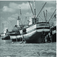
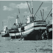
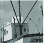
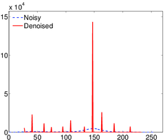
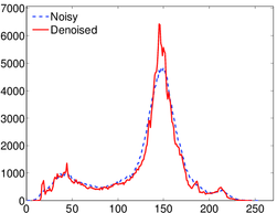
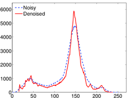
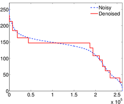
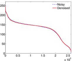
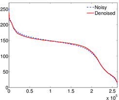
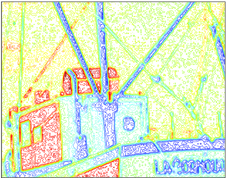
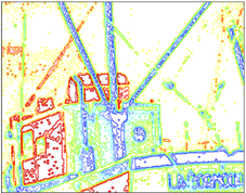
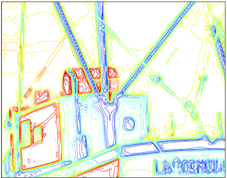
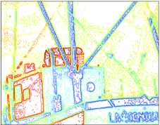
Figure 3: Denoising experiment. Columns: noisy image, Neighborhood, NLM, and Bilateral filters. Rows: noisy image, detail of the image, histograms, decreasing rearrangements, and level curves of image details shown in row 2.

For example, for the Gaussian kernel used in our numerical experiments, it is proven in Theorem 2 that if $v_{0}^{\prime}(t)<0$ then $v_{n}^{\prime}(t)<0$ for all $n$. However, as it may be seen, for instance, in Fig. 3 (fourth row, second column), this property is violated in the discrete framework. Nevertheless, the weaker result $v_{n}^{\prime}(t)\leq 0$ is always observed in the experiments

4.1 Numerical examples for denoising

In the first set of experiments we used the Neighborhood filter for denoising porpouses, and compare it with other related filters: the Bilateral filter,

$$\operatorname{BF}^{h,\rho}u(\mathbf{x})=\frac{1}{C(\mathbf{x})}\int_{\Omega}\textrm{e}^{-\frac{|u(\mathbf{x})-u(\mathbf{y})|^{2}}{h^{2}}}\textrm{e}^{-\frac{|\mathbf{x}-\mathbf{y}|^{2}}{\rho^{2}}}u(\mathbf{y})d\mathbf{y},$$

where $h$ and $\rho$ are positive constants, and

$$C(\mathbf{x})=\int_{\Omega}\exp\left(-|u(\mathbf{x})-u(\mathbf{y})|^{2})h^{-2}\right)\exp\left(-|\mathbf{x}-\mathbf{y}|^{2}\rho^{-2}\right)d\mathbf{y},$$

and the Nonlocal Means filter,

$$\operatorname{NL}^{h,\rho}u(\mathbf{x})=\frac{1}{C(\mathbf{x})}\int_{\Omega}\textrm{e}^{-\frac{G_{\rho}*|u(\mathbf{x}+\cdot)-u(\mathbf{y}+\cdot)|^{2}(0)}{h^{2}}}u(\mathbf{y})d\mathbf{y},$$

where $h>0$, $G_{\rho}$ is a Gaussian kernel of standard deviation $\rho>0$ and

$$C(\mathbf{x})=\int_{\Omega}\exp\left(-G_{\rho}*|u(\mathbf{x}+\cdot)-u(\mathbf{y}+\cdot)|^{2}(0))h^{-2}\right)d\mathbf{y}.$$

Since the usual version of the NF, given by (4), and the version introduced in this article, expressed through the decreasing rearrangement by (8), are equivalent, there is no need of comparison between them.

The denoising properties of these three filters are well known, and a thoroughfull comparison among them (and among other filters) is given in [9]. Here, we are not so interested in deciding which is the best performing denoising algorithm than in analyzing their behavior with respect to the histogram and the decreasing rearrangement redistributions.

We applied the filters on the test images given in the Introduction, see Fig. 1, corrupted with an additive Gaussian white noise of $\text{SNR}=10$, according to the noise measure $\text{SNR}=\sigma(u)/\sigma(\nu)$, where $\sigma$ is the empirical standard deviation, $u$ is the original image, and $\nu$ is the noise.

In Figs. 3 to 5 we show the results of applying these filters to the Boat, the Texture and the Squares images. The columns correspond to: noisy image, Neighborhood filter, Nonlocal means filter, and Bilateral filter. The rows correspond to: image, detail of the image, intensity histograms of noisy and denoised images, decreasing rearrangements of noisy and denoised images, level curves of image details showed in row 2.

Although the Bilateral and the Nonlocal Means filters are applied only once, their execution time is always much larger than that of the iterated Neighborhood filter, for which we used the stopping criterium

$$\frac{|J_{*}(v_{n+1})-J_{*}(v_{n})|}{|J_{*}(v_{n})|}<10^{-5},$$

producing between eight iterations, for the Squares image, and twenty iterations, for the Texture image. We used the same parameter values for $h$ and $\rho$ in all the experiments.

As expected, the best visual result for the natural image is obtained with the Nonlocal Means filter: smoother and with a lower staircaising effect than the others. It is interesting to notice how the absence of local information in the Neighborhood filter produces regions with rapid intensity value changes, for instance in the clouds of the image. The smoothing effect of the local terms in the Bilateral and the NLM filters prevent the formation of this artifact.

A partial explanation of the worse behavior of the NF may be found in the corresponding plots for the histograms and the decreasing rearrangements. While the Bilateral and the NLM filters keep almost unchanged the gray intensity structure of the pixel mass, the NF concentrates most of the mass in few and disconnected values which, in general, is an undesired effect in natural images.

Finally, observe that all the filters produce a level lines shortening, notably the NLM filter.

For the Texture image, similar conclusions may be deduced. In this case, the level lines shortening is specially intense for the NF. The area between the circles is cleaned to one single intensity value, around 225. We may check in the corresponding histograms the large difference between the mass assigned to this value in the different filters. This is a first clue in the consideration of the NF as a segmentation-like filter.

For the synthetic image Squares, the result of applying the NF is almost a perfect image recovery, while the Bilateral and the NLM filters keep always some noise due to the local diffusion. The spatial smoothening effect of the latter work against denoising, for this image.

Let us finally point out to the border effects mentioned after Theorem 3, involving formula (16), and related to the contrast loss induced by the NF. They are clearly visualized in the plots of the decreasing rearrangement of these images. Also the anti-diffusive behavior of the algorithm, captured by the second order term of formula (16) is observed: concave regions induce increase on the iterate while convex regions induce decrease. The result is a steeper slope around the inflexion points at each iteration.

4.2 Numerical examples for segmentation

The intensity histogram, $h_{u}$, of an image $u$ is defined by the measure of its level sets

$$h_{u}(q)=|\{\mathbf{y}\in\Omega:u(\mathbf{y})=q\}|,\quad\text{for }q\in[\min u,\max u].$$

We therefore have the following relationship between the histogram and the distribution function of $u$,

$$m_{u}(q)=\int_{q}^{\max u}h(s)ds.$$

In particular, under regularity assumptions, critical points of the histogram coincides with inflexion points of the distribution function and, hence, of the decreasing rearrangement.

Observe that histogram critical points detection is the base for some segmentation algorithms, see for instance [29, 11, 20, 23]. Due to the discrete nature of computations, finding the maxima of the histogram from where initiating a segmentation procedure is a challenging task.

At this respect, the NF may be seen as a way of detecting histogram maxima, i.e. inflexion points of the decreasing rearrangement, which produces an automatic segmentation with the only tunning of the the window size controlled by $h$.

To demonstrate this capability, we applied the NF to MRI brain segmentation. We used a phantom brain from the Simulated Brain Database [5] with a $9\%$ of additive Riccian noise.

In Fig. 6 we show an axial slice of the volume (initial image) an the corresponding segmentation in four, three and two regions reached by setting $h=17,~{}20,~{}50$, respectively. The contour lines and the decreasing rearrangement are shown too.

In Fig. 7 we show the masks of the segmented regions corresponding to $h=17,~{}20$.

In Fig. 8 we show the grey-white matter segmentation performed with the NF and with other standard packages: Freesurfer [14], FSL [15] and SPM8 [28]. The Dice coincidence coefficient is computed for all the algorithms, see Table 1, showing a good performance of the NF in relation to the more sophisticated algorithms implemented in the mentioned packages. The Dice coefficient is one if a perfect match to the ground truth is attained. Zero, on the contrary.

Although in Fig. 8 we have shown the results for one slice, the NF is applied directly to the whole volume, meaning that the dimension reduction is from a three dimensional space (the space of voxels) to a one dimensional space (the space of level lines measures). Thus, the time execution of the NF is several orders of magnitude lower than the others (a standard volume takes few seconds in a standard laptop).

However, this is no more than a toy example, from where general conclusions can not be inferred.

Table 1: Comparison among several algorithms

	Dice coefficient
	Freesurfer	FSL	SPM	NF
white	0.9490	0.9435	0.9468	0.9563
grey	0.8509	0.8599	0.8835	0.8797

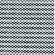
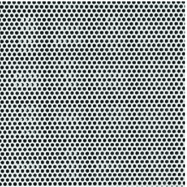
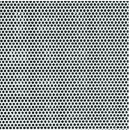
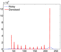
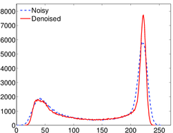
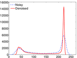
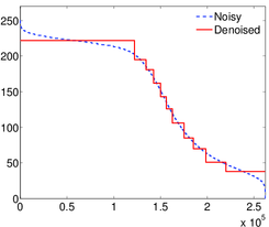
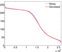
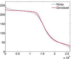
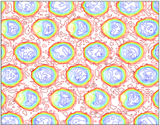
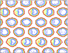
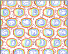
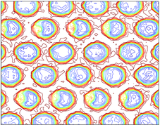
Figure 4: Denoising experiment. Columns: noisy image, Neighborhood, NLM, and Bilateral filters. Rows: noisy image, detail of the image, histograms, decreasing rearrangements, and level curves of image details shown in row 2.

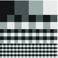
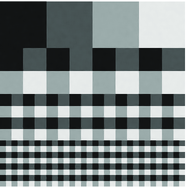
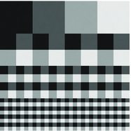
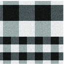
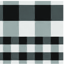
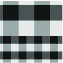
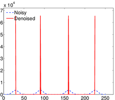
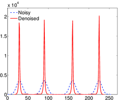
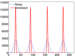
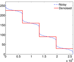
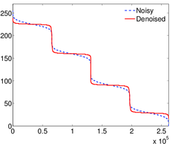
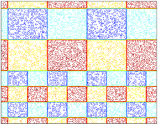
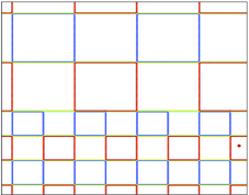
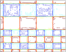
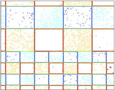
Figure 5: Denoising experiment. Columns: noisy image, Neighborhood, NLM, and Bilateral filters. Rows: noisy image, detail of the image, histograms, decreasing rearrangements, and level curves of image details shown in row 2.

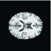
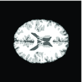
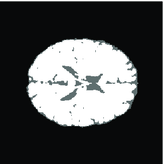
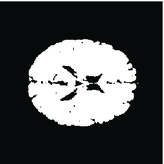
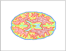
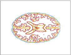
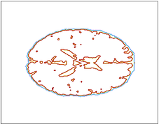
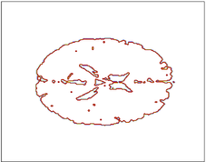
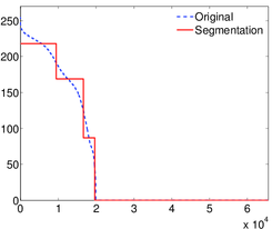
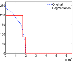
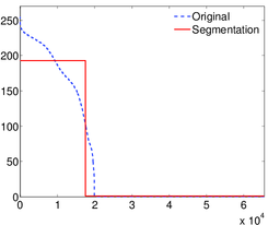
Figure 6: Segmentation experiment. Results of applying the Neighborhood filter with several values of the window size $h$. Rows: Image, level curves and decreasing rearrangement, showing the number of segmented regions (flat regions). Columns: Image, results of applying the NF with $h=17$, $h=20$, and $h=50$, respectively.

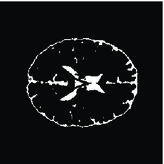
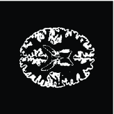
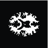
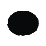
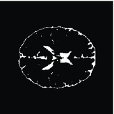
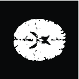
Figure 7: Segmentation experiment. Masks of the segmented regions. First row: $h=17$. The NF produces four regions, corresponding to background, dura-mater and ventricles, grey matter and white matter. Second row: $h=20$. The NF produces three regions, corresponding to background, duramatter and ventricles, grey plus white matter.

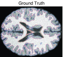
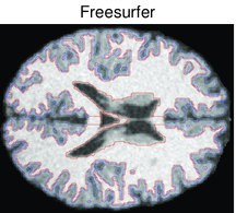
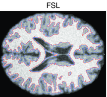
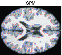
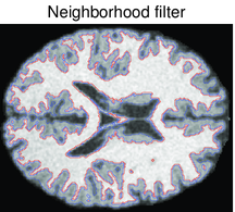
Figure 8: Segmentation experiment. Details of the segmentation produced with several MRI standard packages and with the Neighborhood filter. See Table 1 for details.

5 Summary

In this paper we introduced the use of the decreasing rearrangement to express nonlinear and nonlocal filters in terms of integral operators in the one-dimensional space $[0,|\Omega|]$.

We have proved properties related to the Neighborhood filter nonlinear iterative scheme. In particular, geometric properties like the invariance of level sets and the performance of the filter as a contrast change.

We have also proven a detailed qualitative behavior of the iterations as a power expansion in terms of the window size, and with coefficients which depend on up to second order derivatives of the iterations. This allowed us to distinguish two kind of effects of the filtering process: an anti-diffusive effect of shock-filter type, and a contrast loss effect.

Motivated by the possible piece-wise constant steady state of the discrete problem, we have illustrated the interpretation of the filter as a segmentation algorithm, indeed connected to other techniques involving the histogram thresholding.

The main conclusion of our work is that, for certain kind of images, among which those having concentrated their pixel mass around few intensity levels, the NF is appropriate both as a denoising and as a histogram-maxima based segmentation algorithm. The execution time of its rearranged version clearly out-performs those of other algorithms. However, for other kind of images, specially those with a relatively flat histogram, the results of the NF are poor.

6 Acknowledgments

The authors thank to the anonymous reviewers for their interesting comments and suggestions, which have notably contributed to the improvement of our work.

The authors are partially supported by the Spanish DGI Project MTM2010-18427.

References

- [1] Álvarez L, Mazorra L (1994) Signal and image restoration using shock filters and anisotropic diffusion. Siam J Numer Anal 31(2):590–605
- [2] Álvarez L, Lions PL, Morel JM (1992) Image selective smoothing and edge detection by nonlinear diffusion. ii. Siam J Numer Anal 29(3):845–866
- [3] Barash D (2002) Fundamental relationship between bilateral filtering, adaptive smoothing, and the nonlinear diffusion equation. IEEE T Pattern Anal 24(6):844–847
- [4] Barash D, Comaniciu D (2004) A common framework for nonlinear diffusion, adaptive smoothing, bilateral filtering and mean shift. Image Vision Comput 22(1):73–81
-
[5]
Brainweb,
http://brainweb.bic.mni.mcgill.ca/brainweb,
Vol.t1_icbm_normal_1mm_pn9_rf20_resampled_brain.nii.gz - [6] Buades A, Coll B, Morel JM (2005) A review of image denoising algorithms, with a new one. Multiscale Model Sim 4(2):490–530
- [7] Buades A, Coll B, Morel JM (2006a) Neighborhood filters and pde’s. Numer Math 105(1):1–34
- [8] Buades A, Coll B, Morel JM (2006b) The staircasing effect in neighborhood filters and its solution. IEEE T Image Process 15(6):1499–1505
- [9] Buades A, Coll B, Morel JM (2010) Image denoising methods. a new nonlocal principle. Siam Rev 52(1):113–147
- [10] Caselles V, Monasse P (2010) Geometric description of images as topographic maps. Springer
- [11] Chang CI, Du Y, Wang J, Guo SM, Thouin P (2006) Survey and comparative analysis of entropy and relative entropy thresholding techniques. In: Vision, Image and Signal Processing, IEE Proceedings-, IET, vol 153, pp 837–850
- [12] Collins DL, Zijdenbos AP, Kollokian V, Sled JG, Kabani NJ, Holmes CJ, Evans AC (1998) Design and Construction of a Realistic Digital Brain Phantom. IEEE T Medical Imaging 17(3):463–468
- [13] Elad M (2002) On the origin of the bilateral filter and ways to improve it. Ieee T Image Process 11(10):1141–1151
- [14] Freesurfer http://freesurfer.net
- [15] FMRIB Software Library http://fsl.fmrib.ox.ac.uk/fsl/fslwiki
- [16] Gilboa G, Osher S (2008) Nonlocal operators with applications to image processing. Multiscale Model Sim 7(3):1005–1028
- [17] Kindermann S, Osher S, Jones PW (2005) Deblurring and denoising of images by nonlocal functionals. Multiscale Model Sim 4(4):1091–1115
- [18] Kwan RK-S, Evans AC, Pike GB (1999) MRI simulation-based evaluation of image-processing and classification methods. IEEE T Medical Imaging 18(11):1085–97
- [19] Lieb EH, Loss M (2001) Analysis, vol 4. American Mathematical Soc.
- [20] Nath S, Agarwal S, Kazmi QA (2011) Image histogram segmentation by multi-level thresholding using hill climbing algorithm. Int J Comput Appl 35(1)
- [21] Perona P, Malik J (1990) Scale-space and edge detection using anisotropic diffusion. IEEE T Pattern Anal 12(7):629–639
- [22] Peyré G (2008) Image processing with nonlocal spectral bases. Multiscale Model Sim 7(2):703–730
- [23] Qin K, Xu K, Liu F, Li D (2011) Image segmentation based on histogram analysis utilizing the cloud model. Comput Math Appl 62(7):2824–2833
- [24] Rakotoson JM (2008) Réarrangement Relatif: Un instrument destimations dans les problčmes aux limites, vol 64. Springer
- [25] Rudin LI, Osher S, Fatemi E (1992) Nonlinear total variation based noise removal algorithms. Physica D 60(1):259–268
- [26] Singer A, Shkolnisky Y, Nadler B (2009) Diffusion interpretation of nonlocal neighborhood filters for signal denoising. SIAM J Imaging Sci 2(1):118–139.
- [27] Smith SM, Brady JM (1997) Susan. a new approach to low level image processing. Int J Comput Vision 23(1):45–78
- [28] Statistical Parametric Mapping (SPM) http://www.fil.ion.ucl.ac.uk/spm
- [29] Tobias OJ, Seara R (2002) Image segmentation by histogram thresholding using fuzzy sets. IEEE T Image Process 11(12):1457–1465
- [30] Tomasi C, Manduchi R (1998) Bilateral filtering for gray and color images. In: Sixth International Conference on Computer Vision, 1998, IEEE, pp 839–846
- [31] Yaroslavsky LP (1985) Digital picture processing. An introduction. Springer Verlag, Berlin
- [32] Yaroslavsky LP, Eden M (2003) Fundamentals of Digital Optics. Birkhäuser, Boston