On a singular perturbation problem arising in the theory of Evolutionary Distributions

Abstract

Evolution by Natural Selection is a process by which progeny inherit some properties from their progenitors with small variation. These properties are subject to Natural Selection and are called adaptive traits and carriers of the latter are called phenotypes. The distribution of the density of phenotypes in a population is called Evolutionary Distributions (ED). We analyze mathematical models of the dynamics of a system of ED. Such systems are anisotropic in that diffusion of phenotypes in each population (equation) remains positive in the directions of their own adaptive space and vanishes in the directions of the other’s adaptive space. We prove that solutions to such systems exist in a sense weaker than the usual. We develop an algorithm for numerical solutions of such systems. Finally, we conduct numerical experiments—with a model in which populations compete—that allow us to observe salient attributes of a specific system of ED.

1 Introduction

The—by now discipline—of Evolution by Natural Selection Darwin and Wallace (1858), can be distilled to three principles: (i) inheritance with (ii) variation (called mutations) and (iii) natural selection. Phenotypes are traditionally defined as organisms that display some traits. Traits may be identified with color of skin, height, speed of running, length of a molecule of protein, volume of cells and so on. We use a restricted definition of phenotypes, namely an organism that displays some trait that is subject to natural selection. With abuse of the English language, we call these adaptive traits. For example, an adaptive trait of Polar bears may be the thickness of hair in their fur, where length of hair is presumably inherited.

Now consider the speed of running of prey to be an adaptive trait. Assume that different values of speed are inherited with some variation and is subject to natural selection. Then the speed of running is an adaptive trait. Three issues of interest emerge: Firstly, a value of a trait is an attribute of an organism. Secondly, some variation in these values is not “recognized” as such by natural selection. In our example of speed of running, selection influences survival of those prey that run at, say, $20$ km/hr and those that run at $22$ km/hr equally. This may be so, even when these two different speeds are inherited. Ergo, a value of an adaptive trait is in fact a set of values. And this set identifies a subpopulation made of organisms that belong to a single phenotype where the population is made of phenotypes that carry all values of the adaptive trait. We shall get to the third issue in a moment.

Mathematical models of evolution may be cast via differential equations that are either deterministic or stochastic. Starting with individual-based models is useful for one can construct such models based on first principles. In such models, particles may represent single organisms that may be classified as phenotypes—they exhibit particular values of adaptive traits. Particles may also represent a subpopulation of a phenotypes; namely a set of phenotypes that are lumped into a single subpopulation—of population of all phenotypes—based on the granularity of natural selection. Granularity refers to the idea that in acting upon phenotypes, certain range of values of adaptive traits are indistinguishable by natural selection. This range defines a subpopulation of phenotypes which in fact represents the unit of natural selection.

In modeling evolution by natural selection, one often wishes to switch from individual-based to PDE-based approach. One then begins with an individual-based model, and assumes that the number of particles, $N\rightarrow$ $\infty$. The change of approach—from individual-based to PDE-based—requires justification.

In a nutshell, one begins with a definition of some property that is represented by a particle. In our case, such property consists of values of an adaptive trait. In the context of evolution by natural selection, the dynamics of values of such property are represented by changes in the frequency of such values in a population.

Next, one passes from a space-discrete Lagrangian version of the dynamics to space-continuous Eulerian version. In passing, one is faced with two problems:

Firstly, showing that the counting measure corresponding to the sequence defined by the $N$-particles system as $N\to\infty$ converges to a continuous limit measure. This convergence must be with respect to average values of adaptive traits. Under appropriate regularity conditions, it can be shown that this limit satisfies a PDE-based problem.

Secondly, proving that the limiting evolution PDE, along with appropriate boundary conditions and initial data, is a well-posed problem. Furthermore, that the solution to the problem inherits the essential properties—such as positiveness and boundedness—of the discrete measures,

The first problem, namely that of showing the convergence to a continuous process, has been addressed by Champagnat et al (2006, 2008) for the adaptive evolution of a single populations. Similar mathematical problems have been addressed in spatial dynamics of population Oelschläger (1989); Morale et al (2005); Capasso and Morale (2008); Lachowicz (2008), the theory of chemotaxis and phototaxis Stevens (2000); Levy and Requeijo (2008), and flow in porous medium Oelschläger (1990, 2002).

The second problem relates to solution of a uniformly parabolic ED. Two approaches were taken to derive these parabolic equations—one by Champagnat et al (2006, 2008) and the other by Cohen (2011); Cohen and Galiano (2013). The former applies to a single ED, the latter to a system of ED. The approach employed by Cohen (2011); Cohen and Galiano (2013) stems from the original work by Kimura (1965).

When ED is considered as a system of parabolic ED, the resulting PDE problem is no longer uniformly parabolic, and in fact has a peculiar structure. To understand the lack of uniform parabolicity of the system of PDEs arising in a multipopulation model, let us recall the essential assumptions of the model: (i) selection affects the dynamics of coevolving populations through mortality—that changes the frequency of subpopulations of phenotypes; and (ii) selection and birth are instantaneous events. Consequently, selection and birth are independent events. It follows that mutations, as they should, are random and mutations in each coevolving population occur in a separate (from other populations) so-called adaptive space.

For example, populations of prey and predators may evolve each in an adaptive space made of a single dimension, say, speed of running. Then, through selection, changes in the frequency of phenotypes on the trait value of prey will, in general, induce changes in the frequency of phenotypes along the trait values of predators and vice versa. Therefore, population densities of prey and predators will be affected by the distribution of phenotypes along trait values of their own as well as by those of the other population.

However, mutations in each population occur in the populations’ adaptive space. Because mutations cause diffusion—along values of the adaptive trait—population densities depend on trait values of both populations but only diffuse with respect to one of them.

In other words, we are faced with a special case of anisotropic diffusion in which diffusion of each population remains positive in the directions of their own adaptive space and vanishes in the directions of the other’s adaptive space.

Recall that the second problem we are faced with is showing that the limiting evolution PDE, along with appropriate boundary conditions and initial data, is a well-posed problem. Chipot and coworkers studied related issues in the framework of the theory of singular perturbation. Chipot and Guesmia (2011) proved existence of solutions for a general class of time-independent boundary value problems. They also proved existence and some additional properties of solutions for a particular case of a nonlocal evolution boundary value problem. The problems they studied addressed a single equation; we address a system of equations. Yet, we fundamentally rely on their work.

The complexity of the dynamics of evolution implies that exact solutions to the problem in terms of elementary functions are not available. Even analytical qualitative properties of solution are hard to obtain. Thus, in Section (4), we introduce a numerical discretization of the problem under the Finite Element Method framework. Then, we construct some numerical experiments to observe salient features of the system of ED that cannot be observed otherwise. We also use the numerical experiments to draw conclusions about potential dynamics of evolution under such peculiar systems. See Galiano and Velasco (2011); Galiano (2011, 2012) for related numerical approaches.

2 Mathematical model

Consider a population in which individuals give birth and die at rates that are determined by values of an adaptive trait, $\mathbf{x}$, that they exhibit (a so-called phenotype) and by interactions with other phenotypes. The population is characterized at any time $t$ by the finite counting measure

$$\nu_{t}=\sum_{j=1}^{N(t)}\delta_{\mathbf{x}_{t}^{j}}$$

where $\delta_{\mathbf{x}}$ is the Dirac measure at $\mathbf{x}$. The measure $\nu_{t}$ describes the distribution of phenotypes over the trait space at time $t$. Here $N(t)$ is the total number of phenotypes alive at time $t$, and $\mathbf{x}_{t}^{1},\ldots,\mathbf{x}_{t}^{N(t)}$ denote the values of an adaptive trait—which we identify with individuals (or particles).

Let $K$ be the initial number of individuals and define a normalized population process by

$$X_{t}^{K}=\frac{1}{K}\nu_{t}^{K}.$$

It can be shown that if the initial condition $X_{0}^{K}=\nu_{0}^{K}/K$ converges to a finite deterministic measure with density $u_{0}$ as $K\to\infty$, then under suitable assumptions about the dynamics of the discrete process $\nu_{t}$—see Champagnat et al (2006) for details—the limit of $X_{t}^{K}$ converges in law to a deterministic measure with density $u$ satisfying the following integro-differential equation

$$\partial_{t}u(t,\mathbf{x})=\big{(}(1-\mu(\mathbf{x})) b(\mathbf{x},V*u(t,\mathbf{x}))-d(\mathbf{x},U*u(t,\mathbf{x}))\big{)}u(t,\mathbf{x})$$ (1)

$$+\int_{\mathbb{R}^{d}}\mu(\mathbf{y})M(\mathbf{y},\mathbf{x}-\mathbf{y})b(\mathbf{x},V*u(t,\mathbf{y}))u(t,\mathbf{y})d\mathbf{y}.$$

Here, $U$ and $V$ denote interaction kernels affecting mortality and reproduction, respectively. Functions $d$ and $b$ define the death and birth rate, respectively, of individuals with trait $\mathbf{x}$, whereas $\mu(\mathbf{x})$ is the probability that an offspring produced by a phenotype with trait-value $\mathbf{x}$ carries a value of the adaptive trait that had mutated. The function $M(\mathbf{x},\mathbf{z})$ encapsulates the so-called mutation kernel. It reflects the fact that trait values of progeny, $\mathbf{x}+\mathbf{z}$, differ from those of the progenitor with trait value $\mathbf{x}$ (this, in fact, is the definition of mutations). As noticed by Champagnat et al (2006), (1) is an extension of Kimura’s equation Kimura (1965).

When the values of mutations are small and are distributed systematically (that is according to some probability density), the nonlocal equation (1) may be approximated by

$$\partial_{t}u(t,\mathbf{x})-\frac{1}{2}\Delta\big{(}\mu(\mathbf{x})\varepsilon^{2}(\mathbf{x})u(t,\mathbf{x})\big{)} = u(t,\mathbf{x})\big{(}(1-\mu(\mathbf{x}))b(x,V*u(t,\mathbf{x}))-$$

$$d(x,U*u(t,\mathbf{x}))\big{)},$$

where $\varepsilon(\mathbf{x})\geq\varepsilon_{0}>0$ is the second moment of $M$. Observe that, because adaptive traits represent biological attributes, the set of their values, $\Omega\subset\mathbb{R}^{d}$, must be bounded. So (2) is assumed to hold in $(0,T)\times\Omega$, for some final time $T>0$. Phenotypes with trait-values outside the boundaries cannot survive; therefore, we prescribe homogeneous Dirichlet boundary conditions

$$u(t,\mathbf{x})=0\quad\text{on }(0,T)\times\partial\Omega.$$

When the dynamics include two populations, the generalization of (2) leads to a system of partial differential equations for the densities phenotypes $u_{1}$ and $u_{2}$ with respect to their corresponding populations. It is here that some subtleties arise, and we introduce them next. But first, some notation.

The open and bounded trait space of each population ($i=1,2$) is denoted by $\Omega_{i}$, with $\Omega_{i}\subset\mathbb{R}^{d_{i}}$. An element of $\Omega_{i}$ is denoted by $\mathbf{x}_{i}$ and is given by its components $\mathbf{x}_{i}=(x_{i}^{1},\ldots,x_{i}^{d_{i}})$. We then write $\Omega=\Omega_{1}\times\Omega_{2}$ and $\mathbf{x}=(\mathbf{x}_{1},\mathbf{x}_{2})$. We use the Laplacian operator restricted to $\Omega_{i}$ and write

$$\Delta_{\mathbf{x}_{i}}u(t,\mathbf{x}):=\sum_{j=1}^{d_{i}}\partial_{x_{j}}^{2}u(t,\mathbf{x}).$$

We now state the problem for two populations thus.

For $i,j=1,2$ and $i\neq j$, find $u_{i}:(0,T)\times\Omega\to\mathbb{R}_{+}$ such that

$$\partial_{t}u_{i}-\Delta_{\mathbf{x}_{i}}\big{(}c_{i}u_{i}\big{)}+F_{i}(\cdot,\cdot,u_{1},u_{2})=0 \text{in }(0,T)\times\Omega,$$ (3)

$$u_{i}=0 \text{on }(0,T)\times\partial\Omega_{i}\times\Omega_{j},$$ (4)

$$u_{i}(0,\cdot)=u_{i0} \text{in }\Omega.$$ (5)

The magnitude and rate of mutations are defined thus:

$$c_{i}(\mathbf{x}_{i})=\frac{1}{2}\mu_{i}(\mathbf{x}_{i})\varepsilon_{i}^{2}(\mathbf{x}_{i})$$ (6)

and the interactions within and among populations—including natural selection—thus

$$F_{i}(t,\mathbf{x},u_{1}(t,\mathbf{x}),u_{2}(t,\mathbf{x}))= -\big{(}(1-\mu_{i}(\mathbf{x}_{i}))u_{i}(t,\mathbf{x})b_{i}(\mathbf{x},V*u_{i}(t,\mathbf{x}))$$ (7)

$$-u_{i}(t,\mathbf{x})d_{i}(\mathbf{x},U*u_{1}(t,\mathbf{x}),U*u_{2}(t,\mathbf{x}))\big{)}.$$

Equations (3) to (7) specify the problem, which we dub $\mathbf{P}$.

Remark 1

From a direct differential approach, the following model was derived in Cohen (2011). For $i=1,\ldots,N$ (number of populations), find $U_{i}:(0,T)\times\Omega\to\mathbb{R}_{+}$ such that

$$\partial_{t}U_{i}\left(\mathbf{x},t\right)-\Delta_{\mathbf{x}_{i}}\Big{(}\tilde{\mu}_{i}(\mathbf{x}_{i})B_{i}(U_{i}(t,\mathbf{x}))\Big{)}=B_{i}(U_{i}(t,\mathbf{x}))-M_{i}(U_{1}(t,\mathbf{x}),U_{2}(t,\mathbf{x})),$$ (8)

for some monotone functions $B_{i}$, and with auxiliary data similar to (4)-(5). Observe that for a suitable choice of $\tilde{\mu}_{i}$, $B_{i}$ and $M_{i}$, Equation (3) may be recasted in the form (8). The solution of (8) was dubbed Evolutionary Distribution Cohen (2005).

3 The main result

In this section we study the well-posedness of a variant of $\mathbf{P}$, which we christen $\mathbf{P}1$, namely:

$$\partial_{t}u_{i}-c_{i}\Delta_{\mathbf{x}_{i}}u_{i}+F_{i}(\cdot,\cdot,u_{1},u_{2})=0 \quad\text{in }Q_{T}=(0,T)\times\Omega,$$ (9)

$$u_{i}=0 \quad\text{on }(0,T)\times\partial\Omega,$$ (10)

$$u_{i}(0,\cdot)=u_{i0} \quad\text{in }\Omega,$$ (11)

for $i=1,2$, where we have used the notation introduced in Section 2.

We rely on the following hypotheses about the data, which we shall refer to as H:

For $i=1,2$,

1. $T\in\mathbb{R}_{+}$ is arbitrarily fixed, and $\Omega_{i}\subset\mathbb{R}^{d_{i}}$ is a bounded set with Lipschitz continuous boundary $\partial\Omega_{i}$.

2. The diffusion coefficients, $c_{i}$, are positive constants.

3. The birth-selection terms $F_{i}:Q_{T}\times\mathbb{R}^{2}_{+}\to\mathbb{R}$ satisfy:

   1. $F_{i}(\cdot,\cdot,s_{1},s_{2})\in L^{\infty}(Q_{T})$ for all $(s_{1},s_{2})\in\mathbb{R}^{2}_{+}$.

   2. $F_{i}(t,\mathbf{x},\cdot,\cdot)$ is Lipschitz continuous in bounded sets of $\mathbb{R}^{2}_{+}$ for a.e. $(t,\mathbf{x})\in Q_{T}$, with $F_{1}(\cdot,\cdot,0,\cdot)=F_{2}(\cdot,\cdot,\cdot,0)=0$.

4. The initial data are non-negative and satisfy $u_{i0}\in L^{\infty}(\Omega)\cap H^{1}_{i0}(\Omega)$, where

   $$H^{1}_{i0}(\Omega)=\left\{\varphi\in H^{1}(\Omega):\varphi=0\text{ on }\Omega_{i}\right\}.$$ (12)

We construct a solution of problem $\mathbf{P}1$, namely $(u_{1},u_{2})$, as a limit of a sequence of solutions of approximated singular perturbed problems, $(u_{1}^{(\varepsilon)},u_{2}^{(\varepsilon)})$. In doing so, we face two main difficulties.

Firstly, the lack of uniform estimates for $\nabla_{\mathbf{x}_{j}}u_{i}^{(\varepsilon)}$ for $i\neq j$, which prevent us from getting a global (in space) formulation of a weak solution of $\mathbf{P}1$. As pointed out by Chipot and Guesmia (2009), the regularity of $u_{i}\in L^{2}(0,T;H^{1}_{0}(\Omega))$ can not be guaranteed and therefore, the trace of $u_{i}$ on the boundary $\Omega_{i}\times\partial\Omega_{j}$ is in general not well defined. For examples, see Chipot and Guesmia (2009), where a solution of a time-independent problem is shown to satisfy $u_{i}\in H^{1}_{0}(\Omega_{i})$ concomitant with $u_{i}\notin H^{1}_{0}(\Omega)$. This difficulty also motivates the introduction of the space $H_{i0}^{1}(\Omega)$ in (12). Thus, the notion of weak solution is stated in slices of the domain (see Theorem 1).

Secondly, and, again, due to the lack of uniform estimates for the gradients in the whole domain $\Omega$, strong convergence of the sequence $(u_{1}^{(\varepsilon)},u_{2}^{(\varepsilon)})$ in $L^{2}(Q_{T})\times L^{2}(Q_{T})$ can not be achieved by the usual compactness argument. Yet, this type of convergence is needed to identify the limits of $F_{i}(\cdot,\cdot,u_{1}^{(\varepsilon)},u_{2}^{(\varepsilon)})$. Thus, we resort to a monotonicity property implied by the Lipschitz continuity (H)_3(b) which allows us to perform this identification.

Remark 2

(i) With minor modifications, Theorem 1 may be proved for $\mathbf{x}_{i}$-dependent diffusion coefficients $c_{i}$ under regularity assumptions and the conditions $c_{i}>c_{0}$, for some positive constant $c_{0}$, and $\Delta_{\mathbf{x}_{i}}c_{i}\leq 0$ in $\Omega_{i}$. Indeed, the monotonicity of the elliptic operator in $H^{1}_{0}(\Omega_{i})$ holds under these conditions:

$$-\int_{\Omega_{i}}\big{(}\Delta_{\mathbf{x}_{i}}(c_{i}u_{i})-\Delta_{\mathbf{x}_{i}}(c_{i}\tilde{u}_{i})\big{)}(u_{i}-\tilde{u}_{i}) =\int_{\Omega_{i}}c_{i}|\nabla_{\mathbf{x}_{i}}(u_{i}-\tilde{u}_{i})|^{2}-\frac{1}{2}\int_{\Omega_{i}}|u_{i}-\tilde{u}_{i}|^{2}\Delta_{\mathbf{x}_{i}}c_{i}$$

$$\geq c_{0}\int_{\Omega_{i}}|\nabla_{\mathbf{x}_{i}}(u_{i}-\tilde{u}_{i})|^{2}.$$

(ii) Although to prove our main result on existence of solutions we only need to consider a general Lipschitz domain $\Omega$, in the context of our application this domain is in fact a regular polyhedra due to the choice of independent traits.

In the following theorem we assert the existence of solutions of problem (9)-(11) in a sense weaker than the usual. Indeed, although the components of the solution are globally bounded in $Q_{T}$, the existence of their weak derivatives may be justified only in slices and so the notion of weak solution.

Theorem 1

Assume H. Then problem (9)-(11) has a weak solution $(u_{1},u_{2})$ satisfying, for $i=1,2$, $u_{i}\geq 0$ in $Q_{T}$,

$$u_{i}\in L^{\infty}(Q_{T})\cap L^{2}(0,T;H^{1}_{0}(\Omega_{i}))\cap H^{1}(0,T;L^{2}(\Omega_{i})),$$ (13)

and, for all $\varphi\in L^{2}(0,T;H^{1}_{0}(\Omega_{i}))$ and a.e. $\mathbf{x}_{j}\in\Omega_{j}$ ($j\neq i$)

$$\int_{0}^{T}\int_{\Omega_{i}}\partial_{t}u_{i}\,\varphi+c_{i}\int_{0}^{T}\int_{\Omega_{i}}\nabla_{\mathbf{x}_{i}}u_{i}\cdot\nabla_{\mathbf{x}_{i}}\varphi+\int_{0}^{T}\int_{\Omega_{i}}F_{i}(u_{1},u_{2})\,\varphi=0,$$ (14)

with the initial data being satisfied in the sense that

$$u_{1}(0,\cdot,\mathbf{x}_{2})=u_{10}\quad\text{ in $\Omega_{1}$ for a.e. }\mathbf{x}_{2}\in\Omega_{2},$$

$$u_{2}(0,\mathbf{x}_{1},\cdot)=u_{20}\quad\text{ in $\Omega_{2}$ for a.e. }\mathbf{x}_{1}\in\Omega_{1}.$$

$\Box$

There is no general theory of existence of solutions for problem (9)-(11). Therefore, we introduce the following singular perturbation approximation to the problem. We follow an approach similar to that taken by Chipot and Guesmia (2011) and Chipot et al (2011).

Proof of Theorem 1. We divide the proof in two steps, according to the monotone behavior of functions $F_{i}$.

Step 1. Let us suppose that $F_{i}$ satisfy the following property: for all $(s_{1},s_{2})$ and $(\sigma_{1},\sigma_{2})$ in $\mathbb{R}^{2}_{+}$,

$$\big{(}F_{1}(\cdot,\cdot,s_{1},s_{2})- F_{1}(\cdot,\cdot,\sigma_{1},\sigma_{2})\big{)}(s_{1}-\sigma_{1})+$$ (15)

$$\big{(}F_{2}(\cdot,\cdot,s_{1},s_{2})-F_{2}(\cdot,\cdot,\sigma_{1},\sigma_{2})\big{)}(s_{2}-\sigma_{2})\geq 0$$

a.e. in $Q_{T}$. Then we proceed as follows.

For $i,j=1,2$, $i\neq j$, and some small $\varepsilon>0$, we wish to find $(u_{1}^{(\varepsilon)},u_{2}^{(\varepsilon)})$ such that

$$\int_{0}^{T}<\partial_{t}u_{i},\varphi>+c_{i}\int_{Q_{T}}\nabla_{\mathbf{x}_{i}}u_{i}\cdot\nabla_{\mathbf{x}_{i}}\varphi +\varepsilon\int_{Q_{T}}\nabla_{\mathbf{x}_{j}}u_{i}\cdot\nabla_{\mathbf{x}_{j}}\varphi$$ (16)

$$+\int_{Q_{T}}F_{i}(\cdot,\cdot,u_{1},u_{2})\,\varphi=0,$$

for all $\varphi\in L^{2}(0,T;H^{1}_{0}(\Omega))$, and satisfying the initial data $u_{i}^{(\varepsilon)}(0,\cdot)=u_{i0}^{(\delta)}$, where $u_{i0}^{(\delta)}\in H_{0}^{1}(\Omega)$ and $u_{i0}^{(\delta)}\to u_{i0}$ strongly in $L^{2}(\Omega_{j};H_{0}^{1}(\Omega_{i}))$ as $\delta\to 0$. Up to the last part of the proof, we will consider the parameter $\delta$ fixed, and for clarity, we will not reference it.

The existence of non-negative solutions of the semilinear evolution problem (16) have been established for a large range of functions $F_{i}$, including those satisfying (H)₃ and (15) (see Friedman, 1964, Theorem 9 in Chapter 7). The following regularity holds (Evans, 1998, Theorem 5 in Chapter 7):

$$\begin{array}[]{l}u_{i}^{(\varepsilon)}\in L^{\infty}(Q_{T})\cap C([0,T];L^{2}(\Omega))\cap L^{2}(0,T;H^{2}(\Omega))\cap L^{\infty}(0,T;H_{0}^{1}(\Omega)),\\ \partial_{t}u_{i}^{(\varepsilon)}\in L^{2}(Q_{T}).\end{array}$$ (17)

Recall that, due to property (H)${}_{3\text{(b)}}$, the $L^{\infty}(Q_{T})$ bound implied by (17) is uniform with respect to $\varepsilon$ (Friedman, 1964, Theorem 7 in Chapter 7).

We use $\varphi=u_{i}^{(\varepsilon)}$ as a test function in (16) to get, for $t\in(0,T]$,

$$\frac{1}{2}\int_{\Omega}|u_{i}^{(\varepsilon)}(t,\cdot)|^{2}+c_{i}\int_{Q_{t}}|\nabla_{\mathbf{x}_{i}}u_{i}^{(\varepsilon)}|^{2} +\varepsilon\int_{Q_{t}}|\nabla_{\mathbf{x}_{j}}u_{i}^{(\varepsilon)}|^{2}$$

$$+\int_{Q_{t}}F_{i}(u_{1}^{(\varepsilon)},u_{2}^{(\varepsilon)})u_{i}^{(\varepsilon)}=\frac{1}{2}\int_{\Omega}|u_{i0}^{(\delta)}|^{2}.$$

Summing for $i=1,2$ and using (15)’s property of monotonicity, we attain uniform estimates for

$$\|u_{i}^{(\varepsilon)}\|_{L^{\infty}(0,T;L^{2}(\Omega))},\quad\|\nabla_{\mathbf{x}_{i}}u_{i}^{(\varepsilon)}\|_{L^{2}(Q_{T})},\quad\sqrt{\varepsilon}\|\nabla_{\mathbf{x}_{j}}u_{i}^{(\varepsilon)}\|_{L^{2}(Q_{T})},$$ (18)

implying the existence of some $u_{i}\in L^{2}(Q_{T})$ such that, for a subsequence (not relabeled) we have that

$$u_{i}^{(\varepsilon)}\to u_{i},\quad\nabla_{\mathbf{x}_{i}}u_{i}^{(\varepsilon)}\to\nabla_{\mathbf{x}_{i}}u_{i},\quad\varepsilon\nabla_{\mathbf{x}_{j}}u_{i}^{(\varepsilon)}\to 0$$ (19)

weakly in $L^{2}(Q_{T})$, and

$$u_{i}^{(\varepsilon)}\to u_{i}\quad\text{weakly $*$ in }L^{\infty}(Q_{T}).$$ (20)

In addition, by smoothing-approximation procedure on $\partial_{t}u_{i}^{(\varepsilon)}$, we find (see (Evans, 1998, Theorem 5 in Chapter 7))

$$\|\partial_{t}u_{i}^{(\varepsilon)}\|_{L^{2}(Q_{T})}\leq C\big{(}\|F_{i}(\cdot,\cdot,u_{1}^{(\varepsilon)},u_{2}^{(\varepsilon)}\|_{L^{2}(Q_{T})})+\|u_{i0}^{(\delta)}\|_{H^{1}(\Omega))}\big{)},$$ (21)

for some constant $C>0$ independent of $\varepsilon$. In view of (18) and the continuity of $F_{i}$ stated in (H)${}_{3(\text{b})}$, we also find that $\|\partial_{t}u_{i}^{(\varepsilon)}\|_{L^{2}(Q_{T})}$ is uniformly bounded, implying

$$\partial_{t}u_{i}^{(\varepsilon)}\to\partial_{t}u_{i}\quad\text{weakly in }L^{2}(Q_{T}).$$ (22)

Observe that (19) and (22) permit us to pass to the limit $\varepsilon\to 0$ in the linear terms of (16), with the identification $u_{i}=\lim_{\varepsilon\to 0}u_{i}^{(\varepsilon)}$. However, this is not the case for the nonlinear terms involving $F_{i}(\cdot,\cdot,u_{1}^{(\varepsilon)},u_{1}^{(\varepsilon)})$, for which a stronger sense of convergence is needed to identify their limits. In any case, the $L^{\infty}(Q_{T})$ uniform bounds of $u_{i}^{(\varepsilon)}$ imply, see Evans (1990), the existence of $\tilde{F}_{i}\in L^{\infty}(Q_{T})$ such that

$$F_{i}(\cdot,\cdot,u_{1}^{(\varepsilon)},u_{2}^{(\varepsilon)})\to\tilde{F}_{i},$$ (23)

weakly $*$ in $L^{\infty}(Q_{T})$. Taking the limit $\varepsilon\to 0$ in (16) we find that $u_{i}$ satisfies

$$\int_{Q_{T}}\partial_{t}u_{i}\,\varphi+c_{i}\int_{Q_{T}}\nabla_{\mathbf{x}_{i}}u_{i}\cdot\nabla_{\mathbf{x}_{i}}\varphi+\int_{Q_{T}}\tilde{F}_{i}\,\varphi=0,$$ (24)

for all $\varphi\in L^{2}(0,T;H^{1}_{0}(\Omega))$.

To deduce the convergence $u_{i}^{(\varepsilon)}\to u_{i}$ in a stronger sense, we apply the monotonicity that is afforded us by assumption (15). Let

$$I_{i}^{(\varepsilon)}= \int_{Q_{t}}\Big{(}(u_{i}^{(\varepsilon)}-u_{i})\partial_{t}(u_{i}^{(\varepsilon)}-u_{i})+c_{i}\nabla_{\mathbf{x}_{i}}(u_{i}^{(\varepsilon)}-u_{i})\cdot\nabla_{\mathbf{x}_{i}}(u_{i}^{(\varepsilon)}-u_{i})$$

$$+\varepsilon\nabla_{\mathbf{x}_{j}}u_{i}^{(\varepsilon)}\cdot\nabla_{\mathbf{x}_{j}}u_{i}^{(\varepsilon)}+(u_{i}^{(\varepsilon)}-u_{i})\big{(}F_{i}(\cdot,\cdot,u_{1}^{(\varepsilon)},u_{2}^{(\varepsilon)})-F_{i}(\cdot,\cdot,u_{1},u_{2})\big{)}\Big{)}.$$

On the one hand, using (H)${}_{\text{3(c)}}$ we find

$$I_{1}^{(\varepsilon)}+I_{2}^{(\varepsilon)}\geq\sum_{i=1}^{2}\Big{(}\int_{\Omega}\big{(}|u_{i}^{(\varepsilon)}(t,\cdot)-u_{i}(t,\cdot)|^{2}+c_{i}\int_{Q_{t}}|\nabla_{\mathbf{x}_{i}}(u_{i}^{(\varepsilon)}-u_{i})|^{2}+\varepsilon\int_{Q_{t}}|\nabla_{\mathbf{x}_{j}}u_{i}^{(\varepsilon)}|^{2}\Big{)}.$$ (25)

On the other hand, expanding $I_{i}^{(\varepsilon)}$ and using the problem satisfied by $(u_{1}^{(\varepsilon)},u_{2}^{(\varepsilon)})$, i.e. (16), we find

$$I_{i}^{(\varepsilon)}=\int_{Q_{t}}\Big{(}-u_{i}^{(\varepsilon)}\partial_{t}u_{i}-u_{i}\partial_{t}u_{i}^{(\varepsilon)}+u_{i}\partial_{t}u_{i}-2c_{i}\nabla_{\mathbf{x}_{i}}u_{i}^{(\varepsilon)}\cdot\nabla_{\mathbf{x}_{i}}u_{i}+c_{i}\nabla_{\mathbf{x}_{i}}u_{i}\cdot\nabla_{\mathbf{x}_{i}}u_{i}$$

$$-u_{i}^{(\varepsilon)}F_{i}(\cdot,\cdot,u_{1},u_{2})-u_{i}F_{i}(\cdot,\cdot,u_{1}^{(\varepsilon)},u_{2}^{(\varepsilon)})+u_{i}F_{i}(\cdot,\cdot,u_{1},u_{2})\Big{)}.$$

Taking $\varepsilon\to 0$ and using the convergence properties (19) and (22), and the problem satisfied by $(u_{1},u_{2})$, i.e. (24), we obtain $I_{i}^{(\varepsilon)}\to 0$. Therefore, we deduce from (25) the convergences

$$u_{i}^{(\varepsilon)}\to u_{i},\quad\nabla_{\mathbf{x}_{i}}u_{i}^{(\varepsilon)}\to\nabla_{\mathbf{x}_{i}}u_{i}\quad\text{and}\quad\varepsilon\nabla_{\mathbf{x}_{j}}u_{i}^{(\varepsilon)}\to 0,$$ (26)

strongly in $L^{2}(Q_{T})$. We may now go back to (23) and identify $\tilde{F}_{i}$ as the strong limit in $L^{2}(Q_{T})$ of $F_{i}(\cdot,\cdot,u_{1}^{(\varepsilon)},u_{2}^{(\varepsilon)})$, as $\varepsilon\to 0$. Hence, (24) becomes

$$\int_{Q_{T}}\partial_{t}u_{i}\,\varphi+c_{i}\int_{Q_{T}}\nabla_{\mathbf{x}_{i}}u_{i}\cdot\nabla_{\mathbf{x}_{i}}\varphi+\int_{Q_{T}}F_{i}(\cdot,\cdot,u_{1},u_{2})\,\varphi=0,$$

for all $\varphi\in L^{2}(0,T;H^{1}_{0}(\Omega))$. Observe that due to (22) we also have $u_{i}(0,\cdot)=u_{i0}^{(\delta)}$ a.e. in $\Omega$.

Finally, we justify the passing to the limit $\delta\to 0$. Consider test functions of the form $\varphi(t,\mathbf{x})=\varphi_{i}(t,\mathbf{x}_{i})\varphi_{j}(\mathbf{x}_{j})$, with $\varphi_{i}\in L^{2}(0,T;H_{0}^{1}(\Omega_{i}))$ and $\varphi_{j}\in H^{1}_{0}(\Omega_{j})$, for $i,j=1,2$, $i\neq j$. By density, we deduce that a.e. in $\Omega_{j}$,

$$\int_{0}^{T}\int_{\Omega_{i}}\partial_{t}u_{i}\,\varphi_{i}+c_{i}\int_{0}^{T}\int_{\Omega_{i}}\nabla_{\mathbf{x}_{i}}u_{i}\cdot\nabla_{\mathbf{x}_{i}}\varphi_{i}+\int_{0}^{T}\int_{\Omega_{i}}F_{i}(\cdot,\cdot,u_{1},u_{2})\,\varphi_{i}=0$$

for all $\varphi_{i}\in L^{2}(0,T;H_{0}^{1}(\Omega_{i}))$. We now may use $\varphi_{i}=u_{i}(\cdot,\cdot,\mathbf{x}_{j})$ and (a regularization of) $\varphi_{i}=\partial_{t}u_{i}(\cdot,\cdot,\mathbf{x}_{j})$, for a.e. $\mathbf{x}_{j}\in\Omega_{j}$, to obtain similar estimates to those for the problem stated in the whole $\Omega$, e.g. (18) and (21).

These estimates may be obtained independently of $\delta$ due to the regularity $u_{i0}\in H^{1}_{i0}(\Omega)$ given in assumption (H)₄, and the convergence $u_{i0}^{(\delta)}\to u_{i0}$ strongly in $L^{2}(\Omega_{j};H_{0}^{1}(\Omega_{i}))$. Since the monotonicity properties hold as well, the passing to the limit and its identification follows.

Step 2. If $F_{i}$ do not satisfy property (15), then we introduce the following auxiliary problem. Let $\lambda>0$ be a constant to be chosen. Under the change of unknowns $u_{i}(t,x)=\text{e}^{\lambda t}U_{i}(t,x)$ problem (9)-(11) is formally equivalent to

$$\partial_{t}U_{i}-\Delta_{\mathbf{x}_{i}}U_{i}+\hat{F}_{i}(\cdot,\cdot,U_{1},U_{2})=0 \quad\text{in }Q_{T},$$ (27)

$$U_{i}=0 \quad\text{on }(0,T)\times\partial\Omega,$$ (28)

$$U_{i}(0,\cdot)=u_{i0} \quad\text{in }\Omega,$$ (29)

with $\hat{F}_{i}(t,\mathbf{x},s_{1},s_{2})=\lambda s_{i}+\text{e}^{-\lambda t}F_{i}(t,\mathbf{x},\text{e}^{\lambda t}s_{1},\text{e}^{\lambda t}s_{2})$. Let $L$ be an upper bound for the Lipschitz constants of $F_{i}$. Using the Lipschitz continuity (H)₂, we obtain

$$\big{(}\hat{F}_{1}(s_{1},s_{2})-\hat{F}_{1}(\sigma_{1},\sigma_{2})\big{)}(s_{1}-\sigma_{1})+\big{(}\hat{F}_{2}(s_{1},s_{2})-\hat{F}_{2}(\sigma_{1},\sigma_{2})\big{)}(s_{2}-\sigma_{2})\geq$$

$$\lambda\big{(}(s_{1}-\sigma_{1})^{2}+(s_{2}-\sigma_{2})^{2}\big{)}-L\big{(}(s_{1}-\sigma_{1})^{2}+(s_{2}-\sigma_{2})^{2}+2|s_{1}-\sigma_{1}||s_{2}-\sigma_{2}|\big{)},$$

which is non-negative for $\lambda$ large enough. Therefore, $\hat{F}_{i}$ satisfy the monotonicity condition (15).

Step 1 of this proof ensures the existence of a solution $(U_{1},U_{2})$ to problem (27)-(29) in the weak sense of (14), and with the regularity (13). Then, it is straightforward to check that $u_{i}(t,x)=\text{e}^{\lambda t}U_{i}(t,x)$ solves problem (9)-(11) in an identical weak sense. $\Box$

4 Applications and numerical examples

4.1 Discretization scheme

We follow the ideas of Theorem 1 to construct numerical approximations to problem (9)-(11). We first consider the $\varepsilon-$regularized version given by problem (16), a semilinear parabolic problem for which standard discretization methods may be used, and then produce simulations of the solutions $(u_{1}^{(\varepsilon)},u_{2}^{(\varepsilon)})$ for a collection of decreasing values of $\varepsilon$ to get an idea of the behaviour of solutions to the original unperturbed problem.

For the numerical approximation, we use finite elements in space and backward finite differences in time. More concretely, we consider a quasi-uniform mesh of a rectangle $\Omega\subset\mathbb{R}^{2}$, $\{\mathcal{T}_{h}\}_{h}$, where $h$ represents triangle diameter, and introduce the finite element space of piecewise $\mathbb{P}_{1}$-elements:

$$S^{h}=\{\chi\in\mathcal{C}(\overline{\Omega});\,\chi|_{K}\in\mathbb{P}_{1}\,\text{ for all }K\in\mathcal{T}_{h}\}.$$

The Lagrange interpolation operator, denoted by $\Pi^{h}:\mathcal{C}(\overline{\Omega})\to S^{h}$, from which we define the discrete semi-inner product on $\mathcal{C}(\overline{\Omega})$ is given by

$$(\eta_{1},\eta_{2})^{h}=\int_{\Omega}\Pi^{h}(\eta_{1},\eta_{2}).$$

For the time discretization, we use a uniform partition of $[0,T]$ of time step $\tau$. For $t=t_{0}=0$, set $u_{i0}^{(\varepsilon)}=u_{i0}$. Then, for $n\geq 1$ find $u_{i,n}^{(\varepsilon)}$ such that for $i,j=1,2$ and $i\neq j$,

$$\begin{array}[]{l}\frac{1}{\tau}\big{(}u_{i,n}^{(\varepsilon)}-u_{i,n-1}^{(\varepsilon)},\chi)^{h}+\Big{(}\big{(}c_{i}\partial_{x_{i}}u_{i,n}^{(\varepsilon)},\varepsilon\partial_{x_{j}}u_{i,n}^{(\varepsilon)}\big{)},\nabla\chi\Big{)}+\big{(}F_{i}(u_{1,n-1}^{(\varepsilon)},u_{2,n-1}^{(\varepsilon)}),\chi\big{)}^{h}=0,\end{array}$$ (30)

for every $\chi\in S^{h}$. Since (30) is a nonlinear algebraic problem, we use a fixed point argument to approximate its solution, $(u_{1,n}^{(\varepsilon)},u_{2,n}^{(\varepsilon)})$, at each time slice $t=t_{n}$, from the previous approximation $(u_{1,n-1}^{(\varepsilon)},u_{2,n-1}^{(\varepsilon)})$. Let $u_{i,n}^{\varepsilon,0}=u_{i,n-1}^{(\varepsilon)}$. Then, for $k\geq 1$ the problem is to find $u_{i,n}^{\varepsilon,k}$ such that for all $\chi\in S^{h}$

$$\begin{array}[]{l}\displaystyle\frac{1}{\tau}\big{(}u_{i,n}^{\varepsilon,k}-u_{i,n-1}^{(\varepsilon)},\chi)^{h}+\Big{(}\big{(}c_{i}\partial_{x_{i}}u_{i,n}^{\varepsilon,k},\varepsilon\partial_{x_{j}}u_{i,n}^{\varepsilon,k}\big{)},\nabla\chi\Big{)}+\big{(}F_{i}(u_{1,n}^{\varepsilon,k-1},u_{2,n}^{\varepsilon,k-1}),\chi\big{)}^{h}=0.\end{array}$$

We use a stopping criteria based on the $L^{2}$ relative error between two iterations, i.e.

$$\Big{(}\sum_{i=1,2}\|u_{i,n}^{\varepsilon,k}-u_{i,n}^{\varepsilon,k-1}\|_{L^{2}}^{2}\Big{)}^{1/2}\Big{(}\sum_{i=1,2}\|u_{i,n}^{\varepsilon,k-1}\|_{L^{2}}^{2}\Big{)}^{-1/2}<\text{tol},$$

for values of tol chosen empirically, and set $u_{i,n}^{(\varepsilon)}=u_{i,n}^{\varepsilon,k}$. In some of the experiments we integrate in time until a numerical stationary solution is achieved. This is determined again by an $L^{2}$ relative error measure:

$$\Big{(}\sum_{i=1,2}\|u_{i,n}^{(\varepsilon)}-u_{i,n-1}^{(\varepsilon)}\|_{L^{2}}^{2}\Big{)}^{1/2}\Big{(}\sum_{i=1,2}\|u_{i,n-1}^{(\varepsilon)}\|_{L^{2}}^{2}\Big{)}^{-1/2}<\text{tol}_{S},$$

where $\text{tol}_{S}$ is chosen empirically.

Unless otherwise stated, we use the parameter values of Table 1 in all the experiments. The spatial domain is the square $\Omega=(0,1)\times(0,1)$.

Table 1: Parameter values for the experiments

Parameter	Symbol	Experiment 1
Number of spatial nodes	$N$	$900$
Time step	$\tau$	$1.e-03$
Initial densities	$(u_{10},u_{20})$	$(0.5,0.5)$
Fixed point tolerance	tol	$1.e-03$
Stationary state tolerance	$\text{tol}_{S}$	$1.e-05$
Growth∗	$(\alpha_{1},\alpha_{2})$	$(5,4)$
Selection∗	$\beta_{ij}$	$\left(\begin{array}[]{cc}3&2\\ 2&2\end{array}\right)$

(*) $F_{i}(u_{1},u_{2})=-\big{(}\alpha_{i}u_{i}+u_{i}(\beta_{i1}u_{1}+\beta_{i2}u_{2})\big{)}$

4.2 Numerical examples

Here we show the outcome of competition between two distributions of phenotypes, $u_{1}$ and $u_{2}$, for various values of diffusion coefficients $c_{1}$ and $c_{2}$ and for interactions within and among populations given by

$$F_{i}\left(u_{1},u_{2}\right)=-\Big{(}\alpha_{i}u_{i}+u_{i}\left(\beta_{i1}u_{1}+\beta_{i2}u_{2}\right)\Big{)},$$

see Table 1 for parameter values.

In Experiments 1 and 2 we explore the behavior of solutions for the cases $c_{1}\gg c_{2}$ and $c_{1}=c_{2}$, respectively, directly implementing the discrete version of problem P1, i.e. with the perturbation parameter $\varepsilon=0$. Although Theorem 1 ensures existence of solutions defined in a weaker sense than the usual, we observe good regularity properties in their numerical approximations.

We explore the effect of the magnitude of $\varepsilon$ on the singular perturbation approximation, i.e. to the outcome of (16). Thus, in Experiment 3 we produce numerical approximations of (16) for several decreasing values of $\varepsilon$.

4.2.1 Experiment 1: $c_{1}=0.1,c_{2}=0.01,\varepsilon=0$

Recall that the diffusion coefficients, $c_{i}$ are associated with growth rate of $u_{i}$. In this experiment we implement (14) for different diffusion coefficients $c_{1}=0.1$, $c_{2}=0.01$ in (14) and $\varepsilon=0$ in (16). See Table 1 for parameter value. Figure 1

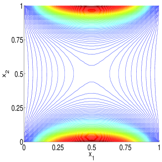
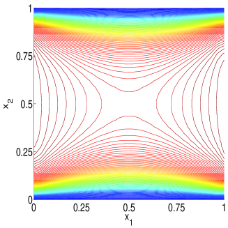
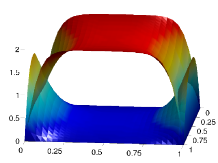
Figure 1: Experiment 1. Top left is the level plot for $u_{1}$ and top right is the level plot for $u_{2}$. The bottom and top surfaces show $u_{1}$ and $u_{2}$ respectively.

reflect the outcome of the distributions $u_{1}$ competing with $u_{2}$.

Here $u_{1}$ shows effect similar to that shown for a single distribution of $u$ in Cohen and Galiano (2013). On the one hand, the distribution $u_{1}$ with $c_{1}=0.1$ ends up with higher density close to the boundaries compared to the center of the values of its adaptive trait, $x_{1}$. On the other, $u_{2}$ reveals trends over their values of adaptive traits $x_{2}$ that mirror those of $u_{1}$. These interactions among distributions of competing populations are reminiscent of the principle of competitive exclusions, where the population with slow diffusion—which is associated with slow growth rate—”winds”.

4.2.2 Experiment 2: $c_{1}=0.1,c_{2}=0.1,\varepsilon=0$

Here we use $c_{1}=0.1$, $c_{2}=0.1$, $\varepsilon=0$ (See Fig. 2).

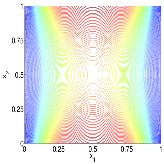
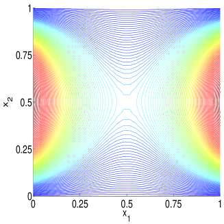
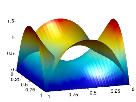
Figure 2: Experiment 2. Top left is the level plot for $u_{1}$ and top right is the level plot for $u_{2}$. The bottom and top surfaces show $u_{1}$ and $u_{2}$ respectively.

As expected, the distributions $u_{1}$ and $u_{2}$ mirror each other in their density over the values of their adaptive traits $x_{1}$ and $x_{2}$. Such symmetric distributions of phenotypes in two populations is not likely to exist in nature.

4.2.3 Experiment 3: $c_{1}=0.1,c_{2}=0.1,\varepsilon>0$ and various boundary conditions

The aim of this experiment is to investigate numerical results for the singular perturbation problem (16).

The proof of Theorem 1 implies the convergence of the sequence of solutions $(u_{1}^{(\varepsilon)},u_{2}^{(\varepsilon)})$ of (16) to a solution of Problem P1. The boundary conditions of problem (16) were set to the Dirichlet conditions.

However, as Figs. 3, 4 and 5 demonstrate, the mixed boundary conditions approximate the actual behavior of the unperturbed problem P1. By mixed boundary conditions we mean

$$u_{i}^{(\varepsilon)}=0 \quad\text{on }(0,T)\times\partial\Omega_{i}\times\Omega_{j}$$

$$\partial_{x_{j}}u_{i}^{(\varepsilon)}=0 \quad\text{on }(0,T)\times\Omega_{i}\times\partial\Omega_{j}$$

for $i,j=1,2$, $i\neq j$.

In Figs. 3, 4 and 5 we show the steady state solutions for several values of $\varepsilon$ for the singular perturbation problem with Dirichlet boundary conditions -DBC- (left panels) and mixed boundary conditions -MBC- (right panels). These solutions approximate those of Experiment 2 (see Fig. 2).

For $\varepsilon=0.1$, the MBC approximate the unperturbed problem while the DBC force the solution to flatten near the boundary of $\Omega$, see Fig. 3.

For $\varepsilon=0.01$, the MBC approximation still shows a declining in the mixed boundary, due to the Neumann boundary condition imposed in these boundaries. The DBC approximation is far from resembling the unperturbed solution (see Fig. 4).

Finally, for $\varepsilon=10^{-10}$, the MBC approximation is indistinguishable from the solution to the unperturbed problem. However, the DBC approximation exhibits a steep boundary layer close to the mixed boundaries which only may disappear in the limit $\varepsilon\to 0$, (see Fig. 5).

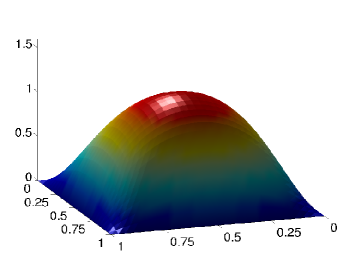
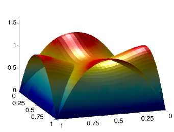
Figure 3: Experiment 3. $\varepsilon=0.1$. Left: Dirichlet. Right: Mixed

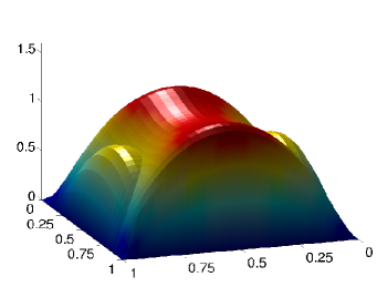
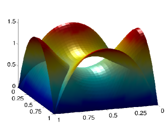
Figure 4: Experiment 3. $\varepsilon=0.01$. Left: Dirichlet. Right: Mixed

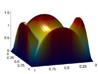
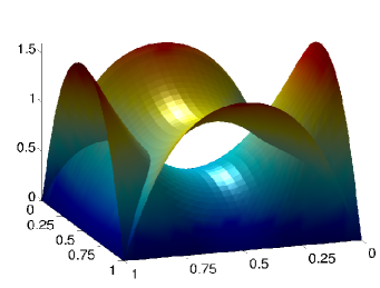
Figure 5: Experiment 3. $\varepsilon=1.e-10$. Left: Dirichlet. Right: Mixed

5 Discussion

Of all the disciplines in the biological sciences, Evolution by Natural Selection is perhaps the only one that can provide answers as to the question of “why” as opposed to “how”.

The dynamics of evolution provide unique challenges to its mathematical modeling through PDE—which when applied to coevolving populations we call a system of ED–in that (among others) (i) diffusion terms in the resulting PDEs are anisotropic and (ii) are determined, solely, by the functions that model growth of populations. Anisotropy in a system of PDEs refers to the property where the diffusion term in each PDE is determined by said PDE only.

As opposed to single ED, the anisotropic property of ED surfaces only in systems of ED. We prove existence of solutions such systems.

Because the structure of systems of ED is unique, numerical algorithms to solve such systems need to be developed; and we did.

Numerical experiments with such algorithms behave as expected from the latter. We conduct factorial experiments that illustrate the effects of the perturbation parameter $\varepsilon$ vis á vis Dirichlet and mixed boundary conditions.

The Dirichlet boundary conditions apply to models of ED. This is so because phenotypes that carry values of adaptive traits outside the boundaries of such traits cannot survive or cannot exist. For example—except for few exceptional cases—organisms whose body temperature is regulated cannot survive if it is (approximately) below $35^{\circ}$C. Neither can they survive for long when their body temperature is (approximately) above $42^{\circ}$C.

The numerical experiments with two competing populations, each with its own adaptive trait, reveal the following: (i) The density of phenotypes mirror each other—this, in spite of the anisotropy; such a pattern surfaces because the ED of the populations interact through the competition term. (ii) Near the boundaries, and as expected, the population that diffuses faster ($c_{1}=0.1$) obtains density higher than the population that diffuses slower ($c_{1}=0.01$). For a single ED, we Cohen and Galiano (2013) obtained dynamics that correspond to the ED with $c_{1}=0.1$ (see left and bottom panels in Figure 1) regardless of the magnitude of the diffusion coefficient. This is so because in a system with a single ED there is no influence (in terms of the diffusion) of another ED that prevents it from achieving high density near the boundaries.

Because $\varepsilon=0$, the results of experiment $2$ reveal symmetric distributions of $u_{1}$ and $u_{2}$; each of the ED correspond to our finding for a single ED Cohen and Galiano (2013).

The results from experiments $3$ to $5$ (given in Figures 3 - 5) illustrate the influence of the perturbation parameter $\varepsilon$ with Dirichlet boundary conditions compared to mix boundary conditions. The right panels of each of the Figures reflect the ever increasing density at the boundaries (compared to the center) of the distribution. The trends in these results correspond to those with the Dirichlet boundary conditions.

References

- Capasso and Morale (2008) Capasso V, Morale D (2008) Rescaling stochastic processes: Asymptotics. In: Multiscale Problems in the Life Sciences, Springer, pp 91–146
- Champagnat et al (2006) Champagnat N, Ferrière R, Méléard S, et al (2006) Unifying evolutionary dynamics: from individual stochastic processes to macroscopic models. Theor Popul Biol 69(3):297–321
- Champagnat et al (2008) Champagnat N, Ferrière R, Méléard S (2008) From individual stochastic processes to macroscopic models in adaptive evolution. Stoch Models 24:2–44
- Chipot and Guesmia (2009) Chipot M, Guesmia S (2009) On the asymptotic behavior of elliptic, anisotropic singular perturbations problems. Commun Pure Appl Anal 8(1):179–193
- Chipot and Guesmia (2011) Chipot M, Guesmia S (2011) On some anisotropic, nonlocal, parabolic singular perturbations problems. Appl Anal 90(12):1775–1789
- Chipot et al (2011) Chipot M, Guesmia S, Sengouga A (2011) Singular perturbations of some nonlinear problems. J Math Sci 176(6):828–842
- Cohen (2005) Cohen Y (2005) Evolutionary distributions in adaptive space. J Appl Math 2005(4):403 – 424
- Cohen (2011) Cohen Y (2011) Evolutionary distributions: producer consumer pattern formation. J Biol Dyn 5:253–267
- Cohen and Galiano (2013) Cohen Y, Galiano G (2013) Evolutionary distributions and competition by way of reaction-diffusion and by way of convolution. Bull Math Biol
- Darwin and Wallace (1858) Darwin C, Wallace A (1858) On the tendency of species to form varieties; and on the perpetuation of varieties and species by natural means of selection. Journal of the Proceedings of the Linnean Society of London Zoology 3:45–62
- Evans (1990) Evans LC (1990) Weak convergence methods for nonlinear partial differential equations. American Mathematical Society, Providence
- Evans (1998) Evans LC (1998) Partial differential equations. American Mathematical Society, Providence
- Friedman (1964) Friedman A (1964) Partial differential equations of parabolic type, vol 196. Prentice-Hall, New Jersey
- Galiano (2011) Galiano G (2011) Modeling spatial adaptation of populations by a time non-local convection cross-diffusion evolution problem. Appl Math Comput 218(8):4587–4594
- Galiano (2012) Galiano G (2012) On a cross-diffusion population model deduced from mutation and splitting of a single species. Comput Math Appl 64(6):1927–1935
- Galiano and Velasco (2011) Galiano G, Velasco J (2011) Competing through altering the environment: A cross-diffusion population model coupled to transport–darcy flow equations. Nonlinear Anal Real World Appl 12(5):2826–2838
- Kimura (1965) Kimura M (1965) A stochastic model concerning the maintenance of genetic variability in quantitative characters. Proc Natl Acad Sci USA 54:731–736
- Lachowicz (2008) Lachowicz M (2008) Lins between microscopic and macroscopic descriptions. In: Multiscale Problems in the Life Sciences, Springer, pp 201–267
- Levy and Requeijo (2008) Levy D, Requeijo T (2008) Modeling group dynamics of phototaxis: from particle systems to pdes. Discrete Contin Dyn Syst Ser B 9(1):103–128
- Morale et al (2005) Morale D, Capasso V, Oelschläger K (2005) An interacting particle system modelling aggregation behavior: from individuals to populations. J Math Biol 50(1):49–66
- Murray (2003) Murray JD (2003) Mathematical Biology I. An introduction, 3rd edn. Springer, New York
- Oelschläger (1989) Oelschläger K (1989) On the derivation of reaction-diffusion equations as limit dynamics of systems of moderately interacting stochastic processes. Probab Theory Related Fields 82(4):565–586
- Oelschläger (1990) Oelschläger K (1990) Large systems of interacting particles and the porous medium equation. J Differential Equations 88(2):294–346
- Oelschläger (2002) Oelschläger K (2002) Simulation of the solution of a viscous porous medium equation by a particle method. SIAM J Numer Anal 40(5):1716–1762
- Stevens (2000) Stevens A (2000) The derivation of chemotaxis equations as limit dynamics of moderately interacting stochastic many-particle systems. SIAM J Appl Math 61(1):183–212