A Gemini/GMOS study of the physical conditions and kinematics of the blue compact dwarf galaxy Mrk 996

Abstract

Aims. We present an integral field spectroscopic study with the Gemini Multi-Object Spectrograph (GMOS) of the unusual blue compact dwarf (BCD) galaxy Mrk 996.

Methods. We show through velocity and dispersion maps, emission-line intensity and ratio maps, and by a new technique of electron density limit imaging that the ionization properties of different regions in Mrk 996 are correlated with their kinematic properties.

Results. From the maps, we can spatially distinguish a very dense high-ionization zone with broad lines in the nuclear region, and a less dense low-ionization zone with narrow lines in the circumnuclear region. Four kinematically distinct systems of lines are identified in the integrated spectrum of Mrk 996, suggesting stellar wind outflows from a population of Wolf-Rayet (WR) stars in the nuclear region, superposed on an underlying rotation pattern. From the intensities of the blue and red bumps, we derive a population of $\sim$473 late nitrogen (WNL) stars and $\sim$98 early carbon (WCE) stars in the nucleus of Mrk 996, resulting in a high $N$(WR)/$N$(O+WR) of 0.19.

We derive, for the outer narrow-line region, an oxygen abundance 12+log(O/H)=7.94$\pm 0.30$ ($\sim$ 0.2 $Z_{\odot}$) by using the direct T_e method derived from the detected narrow [O iii]$\lambda$4363 line. The nucleus of Mrk 996 is, however, nitrogen-enhanced by a factor of $\sim$20, in agreement with previous CLOUDY modeling. This nitrogen enhancement is probably due to nitrogen-enriched WR ejecta, but also to enhanced nitrogen line emission in a high-density environment. Although we have made use here of two new methods - Principal Component Analysis (PCA) tomography and a method for mapping low- and high-density clouds - to analyze our data, new methodology is needed to further exploit the wealth of information provided by integral field spectroscopy.

1 Introduction

The blue compact dwarf (BCD) galaxy Mrk 996 ($M_{B}$ = $-$16.9) is a very unusual galaxy. It stands out from its counterparts because of its extremely large nuclear electron density, of the order of 10⁶ cm^-3 instead of the usual several 100 cm^-3 for H ii regions. Much work has been done to study the unusual physical properties of Mrk 996. Hubble Space Telescope (HST) $V$ and $I$ images by Thuan et al. (1996) show that the bulk of the star formation occurs in a compact, roughly circular, high surface brightness nuclear region of radius  340 pc, with evident dust patches to the north of it. The nucleus (n) is located within an elliptical (E) low surface brightness (LSB) component, so that Mrk 996 belongs to the relatively rare class of nE BCDs (Loose & Thuan 1985). It may also be classified as a Type I H ii galaxy according to Telles et al. (1997). Thuan et al. (1996) found the extended envelope to show a distinct asymmetry. The envelope is more extended to the northeast side than to the southwest side, perhaps the sign of a past merger. This asymmetry is also seen in the spatial distribution of the globular clusters around Mrk 996, seen mainly to the south of the galaxy. The extended LSB component possesses an exponential disc structure with a small scale length of 0.42 kpc. While Mrk 996 does not show an obvious spiral structure in the disc, there is a spiral-like pattern in the nuclear star-forming region, which is no larger than 160 pc in radius. This galaxy has a heliocentric radial velocity of 1622 km s^-1 (Thuan et al. 1999), which gives it a distance of 21.7 Mpc, adopting a Hubble constant of 75 km s^-1 Mpc^-1 and including a very small correction for the Virgocentric flow. Table 1 summarizes the basic information on Mrk 996. At the adopted distance, 1″ corresponds to a linear size of 105 pc.

The UV and optical spectra of the nuclear star-forming region of Mrk 996 (Thuan et al. 1996) show remarkable features, suggesting very unusual physical conditions. The He i line intensities are 2-4 times larger than those in normal BCDs. In the UV range, the N iii] $\lambda$ 1750 and C iii] $\lambda$ 1909 are particularly intense. Moreover, the line width depends on the degree of ionization of the ion. Thus, low-ionization forbidden emission lines such as [O ii] $\lambda$3726,3729, [S ii] $\lambda$6717, 6731, and [N ii] $\lambda$6548, 6584 have narrow widths, similar to those in other H ii regions, while high-ionization emission lines such as the helium lines, the [O iii] $\lambda$4959, 5007, and [Ne iii] $\lambda$3868 nebular lines consist of narrow and broad components, and all auroral lines such as [O iii] $\lambda$4363, [N ii] $\lambda$5755, and [S iii] $\lambda$6312 are broad with line widths of $\geq$ 500 km s^-1. These correlations of line widths with the degree of excitation suggest different ionization zones with very distinct kinematic properties. Thuan et al. (1996) found that the usual one-zone, low-density, ionization-bounded H ii region model cannot be applied to the nuclear star-forming region of Mrk 996 without leading to unrealistic helium and heavy-element abundances. Instead, they showed that a two-zone, density-bounded H ii region model that includes an inner compact region with a central density of  10⁶ cm^-3 (about 4 orders of magnitude greater than the densities of normal H ii regions) together with an outer region with a lower density of $\sim$ 450 cm^-3 (comparable to those of other H ii regions), is needed to account for the observed line intensities. The large density gradient is probably caused by a mass outflow driven by the large population of Wolf-Rayet stars present in the galaxy. The gas outflow motions may account for the line widths of the high-ionization lines originating in the dense inner region being much broader than the low-ionization lines originating in the less dense outer region. The high intensities of [N iii] $\lambda$1750, [C iii] $\lambda$1909, and He i can be understood by collisional excitation of these lines in the high-density region. In the context of this model, the oxygen abundance of Mrk 996 is 12+ log O/H =8.0. If we adopt 12+ log O/H = 8.70 for the Sun (Asplund et al. 2009), then Mrk 996 has a heavy element mass fraction of 0.2 solar. The 2-zone CLOUDY models with element abundance ratios typical of low-metallicity BCDs reproduce well the observed line intensities, except for nitrogen. With an enhancement factor of $\sim$5 or greater, the nitrogen line intensities can be reproduced. Thuan et al. (1996) attribute this nitrogen enhancement to local pollution from Wolf-Rayet stars.

Thuan et al. (2008) have used the Spitzer satellite to study Mrk 996 in the mid-infrared (MIR). They also found that a CLOUDY model that accounts for both the optical and MIR lines requires that they originate in two distinct H ii regions: a very dense H ii region where most of the optical lines arise, with densities declining from  10⁶ cm^-3 at the center to a few hundred cm^-3 at the outer radius of $\sim$ 580 pc, and a H ii region with a density of $\sim$ 300 cm^-3 that is hidden in the optical, but seen in the MIR. The infrared lines arise mainly in the optically obscured H ii region, while they are strongly suppressed by collisional deexcitation in the optically visible one. The presence of the [O iv] 25.89 $\mu$m emission line implies the presence of ionizing radiation as hard as 54.9 eV. This hard ionizing radiation is most likely due to fast radiative shocks propagating in a dense interstellar medium.

Because of the presence in it of distinct ionization zones with different electron densities and kinematic properties, a very dense nuclear high-ionization zone with broad emission lines and a less dense low-ionization zone with narrow emission lines in the circumnuclear region, Mrk 996 is a prime target for observation with the Gemini Multi-object Spectrograph. This allows us to carry out a two-dimensional (2D) study of the kinematics and ionization structure of Mrk 996 with exquisite spatial and spectral resolution. In the same spirit, James et al. (2009) have also recently carried a 2D study of Mrk 996 with the VLT VIMOS integral field unit, although with less spatial and spectral resolution. Those authors found that most of the emission lines of Mrk 996 show two components: a narrow central Gaussian with a full width at half-maximum FWHM$\sim$110 km s^-1 superposed on a broad component with FWHM$\sim$400 km s^-1. The [OIII] $\lambda$4363 and [NII] $\lambda$5755 lines show only a broad component and are detected only in the inner region. The broad line region shows N/H and N/O enhanced by a factor of $\sim$20, while the abundances of the other elements are normal. An oxygen abundance of 12+log(O/H)=8.37, greater than 0.5 that of the Sun, and a very large Wolf-Rayet ($\sim$ 3000) and O star ($\sim$ 150 000) population were derived. A follow-up Chandra study to explore the presence of an intermediate-mass black hole in the heart of Mrk 996 which may account for the presence of the [O iv] 25.89 $\mu$m line was undertaken by Georgakakis et al. (2011). No Active Galactic Nuclei (AGN) were found.

We discuss the observations and the data reduction in Sect. 2. The integrated spectrum is considered in Sect. 3. We discuss here the systems of emission lines with different kinematics, the collisional excitation of hydrogen and helium lines, and the Wolf-Rayet stellar population. The 2D kinematics data are presented in Sect. 4 in the form of velocity and velocity dispersion maps. In Sect. 5 we present a technique to delimit the spatial extent of the high electron density region. In Sect. 6 we apply a recently developed method for exploiting data cubes and extracting uncorrelated physical information, called Principal Component Analysis (PCA) tomography. The 2D description of the physical conditions is presented in Sect. 7 through extinction, electron temperature and density, excitation, and Wolf-Rayet feature maps. We summarize our conclusions in Sect. 8.

Table 1: Basic data on Mrk 996

Parameter	Value
$\alpha$(J2000)	01h27m35$\aas@@fstack{s}$5
$\delta$(J2000)	$-$06°19′36″
Heliocentric velocity [ $\hbox{km}\thinspace\hbox{s}^{-1}$]	1622
$z$	0.0054
Distance [Mpc]	21.7
$C$(H$\beta$)	0.53
$E(B-V)$Gal	0.044

2 Observations and data reduction

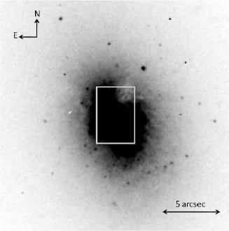
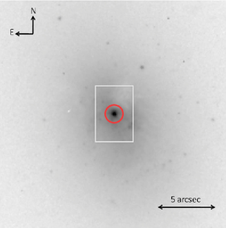
Figure 1: The GMOS 3$\aas@@fstack{\prime\prime}$5$\times$5″ field of view superimposed on the inner 20″ of the HST/F569W image of Mrk 996 from Thuan et al. (1996) The scale and orientation are given. Left: Linear contrast. Right: Logarithmic contrast to emphasize the compact nucleus. The central circle corresponds to the nuclear aperture of 1$\aas@@fstack{\prime\prime}$6 in diameter used in this work.

The observations were obtained with the Gemini Multi-Object Spectrograph (GMOS) (Hook et al. 2004) and the Integral Field Unit (IFU) (Allington-Smith et al. 2002, hereafter GMOS/IFU) at the Gemini South Telescope in Chile. They were made during the nights of October 20, 2008, using the grating B1200$+\_$G5321 (B1200) covering the wavelength region from 3667Å to 5142Å with a spectral resolution of 0.24Å, and of November 6, 2008, using the grating R831$+\_$G5322 (R831) with a spectral resolution of 0.34Å, covering the wavelength region from 5095Å to 7223Å, with an overlap of $\sim$50Å between the red and blue spectral ranges, in the one-slit mode. The GMOS/IFU in this mode composes a pattern of 750 hexagonal elements, each with a projected diameter of 0$\aas@@fstack{\prime\prime}$2, covering a total 3$\aas@@fstack{\prime\prime}$5 $\times$5″ field of view, where 250 of these elements are dedicated to sky observation. The detector is made up of three 2048$\times$4608 CCDs with 13.5 $\mu$m pixels, with a scale of 0$\aas@@fstack{\prime\prime}$073 pixel^-1. The CCDs create a mosaic of 6144$\times$4608 pixels with a small gap of 37 columns between the chips. Figure 1 shows the inner 20″ of the HST Wide Field Camera F569W filter image of Mrk 996 from Thuan et al. (1996) with the location of our GMOS field of view superimposed on it, with a linear contrast (left) and with a logarithmic stretch (right) to emphasize the compact nuclear region.

Table 2 shows the observing log which gives the instrumental setup, the mean airmass and exposure times, the dispersion, the final instrumental resolution ($\sigma_{inst}$=$FWHM_{inst}$/2.355), and the seeing ($FWHM$) of each observation. The data were reduced using the Gemini package version 1.8 inside IRAF. All science exposures, comparison lamps, spectroscopic twilight, and GCAL flats were overscan/bias subtracted and trimmed. The spectroscopic GCAL flats were processed by removing the calibration unit with GMOS spectral response and the uneven illumination of the calibration unit. Twilight flats were used to correct for the illumination pattern in the GCAL lamp flat using the task gfresponse in the GMOS package. The twilight spectra were divided by the response map obtained from the lamp flats and the resulting spectra were averaged in the dispersion direction, giving the ratio of sky to lamp response for each fiber. The final response maps were then obtained by multiplying the GCAL lamp flat by the derived ratio. The resulting extracted spectra were then wavelength calibrated, corrected by the relative fiber throughputs, and extracted. The residual values in the wavelength solution for 40 and 60 points, using a Chebyshev polynomial of the fourth or fifth order, typically yielded rms values of $\sim$0.08Å and $\sim$0.07Å for the red and blue gratings, respectively. The final spectra cover wavelength intervals of $\sim$3667–5142Å and $\sim$5095–7223Å for data taken with the B1200 and R813 gratings, respectively.

Table 2: Observational setup

Observation	Grating	Central Wavelength	Airmass	Exposure Time	Dispersion	$\sigma_{inst}$	Seeing
date		[Å]		[seconds]	[Å/pixel]	[ $\hbox{km}\thinspace\hbox{s}^{-1}$]	[″]
(1)	(2)	(3)	(4)	(5)	(6)	(7)	(8)
2008 Oct 20	B1200	4420	1.64	3$\times$1200	0.23	21.1	0.5
2008 Nov 6	R831	6160	1.22	3$\times$900	0.34	22.8	0.8

The flux calibration was performed using the sensitivity function derived from observations of the star Feige 110 and LTT1020 for both gratings. The 2D data images were transformed into a 3D data cube ($x,y,\lambda$), re-sampled as square pixels with 0$\aas@@fstack{\prime\prime}$1 spatial resolution and corrected for differential atmospheric refraction (DAR) using the gfcube routine. The three cubes with different exposures were combined to produce a single data cube for each grating. The flux maps on selected emission lines, radial velocity, and velocity dispersion maps, as well as 1D spectra of various apertures, were created by an extensive use of QFitsview, developed by Thomas Ott. Both reduced and calibrated data cubes have been made publicly available .

3 Integrated spectrum

3.1 Selecting our extraction apertures

We have simulated apertures for the extraction of the integrated spectrum in order to compare our results with those of the similar IFU VIMOS work of James et al. (2009), as well as those of the HST work of Thuan et al. (1996) on the nuclear spectral properties of this peculiar galaxy. James et al. (2009) used a $1.7\times 2.3$″² aperture for the core region and a $5.3\times 6.3$″² aperture for the outer part outside the core, and Thuan et al. (1996) obtained a nuclear spectrum with a 0$\aas@@fstack{\prime\prime}$86 circular aperture with HST. The results of this simulated aperture analysis indicates that the VIMOS data of James et al. (2009) show similar line ratios for both the narrow and broad components for most lines, but the absolute fluxes are a factor of 4-5 higher than our data for the nuclear aperture. A direct comparison with the outer region was not possible because our field of view ($3.5\times 5.0$ ″²) is slightly smaller than that of VIMOS. On the other hand, our HST simulated aperture fluxes and flux ratios give a good match to those of the HST spectrum of Thuan et al. (1996). Because of the flux discrepancy with the VIMOS data, we have re-reduced the whole data set using the more recent software that was developed by one of us (ERC, responsible for GMOS). We have thus double-checked our measurements by a new and independent data reduction, and confirmed our calibration.

Having established the accuracy of our data reduction, by both internal and external checks, we decided to present the results for the integrated spectrum using a circular aperture of 1$\aas@@fstack{\prime\prime}$6 in diameter, representative of the nuclear region of Mrk 996. This aperture size is consistent with the full width at zero intensity (FWZI) of the point spread function (PSF) of our calibration star, using the same instrument and setup on the same night. The second aperture used in this work contains the outer region, consisting of the spaxels within our field of view, but not considering the inner 1$\aas@@fstack{\prime\prime}$3 radius (5 pixels from the nucleus aperture). Although both apertures used in the present work (the nuclear and the outer regions) are similar to those used by James et al. (2009), ours encompass smaller areas than theirs.

3.2 Systems of emission lines with different kinematics

Figure 2: Integrated GMOS spectrum of the nucleus of Mrk 996 within a 1$\aas@@fstack{\prime\prime}$6 circular aperture for the whole observed spectral range.

In Fig. 2, we show the integrated nuclear spectrum of Mrk 996 over the entire spectral range covered by the two gratings, within a 1$\aas@@fstack{\prime\prime}$6 circular aperture centered on the nucleus. While this aperture is very similar to the core region aperture of James et al. (2009), as mentioned above, it is not identical.

This spectrum has a higher spectral resolution (a factor of $\sim$10 in the blue and of $\sim$4 in the red) and a considerably higher signal-to-noise ratio (S/N) than the spectrum of James et al. (2009). It also covers a larger wavelength range. The spectrum has not been smoothed. The continuum levels of the blue and red parts of the integrated spectrum in the overlapping region at $\sim$ 5100Å match well although the two data cubes were taken on different nights. This, again, confirms our data reduction and calibration. We note that in the bluest part, for $\lambda$ $<$ 4000Å, the continuum is not monotonically increasing to the blue, implying a poorer calibration due to the known low sensitivity of GMOS in that wavelength region. However, the remaining continuum is monotonically increasing from the red to the blue, in agreement with the spectrum of Thuan et al. (1996). By comparison, the continuum in the red part of the James et al. (2009) spectrum is nearly flat, probably indicating the contribution of the more spatially extended red old stellar population, due to the use of a considerably larger aperture (5$\aas@@fstack{\prime\prime}$3 by 6$\aas@@fstack{\prime\prime}$3).

The high spectral resolution of the GMOS/IFU observations allows us to resolve the [O ii] $\lambda$3726, 3729 doublet lines. The hydrogen Balmer lines all show a narrow and a broad component. The total flux in the broad component of H$\alpha$ is comparable to the total flux in its narrow component. The He i lines ($\lambda$4471, $\lambda$5876, $\lambda$6678, $\lambda$7065) are clearly broadened. The broad component is dominant in the [O iii] $\lambda$4363, [N ii] $\lambda$5755, and [S iii] $\lambda$6312 auroral lines, while the low-ionization species [S ii]$\lambda\lambda$ 6717,6731, [O ii]$\lambda\lambda$ 3726,3729, [N ii] $\lambda\lambda$ 6548,6584, and [O i]$\lambda\lambda$ 6300,6363 lines are all narrow, with no broad component. These general trends agree with those discussed by Thuan et al. (1996) and James et al. (2009).

Figure 3: Example of the deblend fitting procedure with the H$\alpha$ line. Upper panel: The integrated profile of the H$\alpha$ line as in Figure 2 (black solid line). The red-dotted line shows the resulting fit to the broad component. The blue-dashed line shows the resulting fit to the narrow component. The integrated fluxes in the broad and narrow components in Table 3 are derived in this manner. Lower panel: residuals to the fit.

Thanks to the high spectral resolution of our data, the narrow and broad components of emission lines are well separated. Therefore, using the IRAF splot routine we first fit the narrow component by a single Gaussian and subtract it from the line profile. Then we fit the broad component again by a single Gaussian. Additionally, very broad low-intensity H$\alpha$ emission is present with a FWZI of $\sim$100Å, suggesting rapid outflow with a velocity of several thousand km s^-1. This low-intensity H$\alpha$ emission was not discussed by James et al. (2009), probably because of the lower S/N of their spectrum. In principle, a multi-Gaussian fitting to emission line profiles should have been used, including more than two components for each line. However, this approach is subjective when more Gaussians are used for profile-fitting, the fit is better, without necessarily reflecting the real physical situation. Additionally, this procedure significantly complicates studies of the kinematic structure. Therefore, we have decided to fit line profiles in the simplest way, each of their narrow and broad components being fitted by a single Gaussian. Fig. 3 shows an example of our deblend fits for deriving our fluxes in our line-fitting procedure. The lower panel shows the residuals of the fit. It can be seen that the broad component is flat on top, rather than being a perfect Gaussian. For the purpose here the measured fluxes are little affected by this deviation. We show in Table 3 the results of the line-fitting for the integrated nucleus spectrum within the 1$\aas@@fstack{\prime\prime}$6 circular aperture . In this table, $\lambda_{0}$ is the rest-frame wavelength and $N_{e}$(crit) is the critical density of the forbidden line. The flux is in units of 100$\times$$F_{nar}$/$F_{nar}$(H$\beta$) for the narrow component and of 100$\times$$F_{br}$/$F_{br}$(H$\beta$) for the broad component; $v(rad)$ is the radial velocity in km s^-1, and $FWHM$ is the line full width at half maximum in km s^-1. Errors in radial velocities are negligible and are not quoted. All measurements were performed by hand with the task splot within IRAF, and also by running non-interactively the profile fitting task fitprofs, providing initial guesses for positions and widths of the lines. The results of these non-interactive fits are, in most cases, identical to our measurements with splot. The advantage is that fitprofs computes error estimates for the fitted parameters by using a Monte Carlo technique that automatically takes into account the properties of our data. The details of this technique is given in the fitprofs help pages. We have chosen a large number of iterations for better error estimates. These are the errors quoted in Table 3. The errors introduced by flat-fielding the data is $<$ 1%. A larger error of 3-4% is introduced when the correction by the relative fiber throughputs is performed (response map). This will result in a 4-5% total error, to be added in quadrature to the listed errors in Table 3.

Table 3: Emission line parameters derived from the integrated spectrum within a 1$\aas@@fstack{\prime\prime}$6 aperture

		$N_{e}$(crit)	Flux			$v(rad)$			$FWHM$
Ion	$\lambda_{0}$	cm-3	narrow	broad		narrow	broad		narrow	broad
$[$O ii$]$	3726.03	4.5$\times$103	92.39$\pm$1.34			1640			135$\pm$7
$[$O ii$]$	3728.82	9.8$\times$102	93.98$\pm$1.35			1634			124$\pm$9
H10	3797.90		6.18$\pm$0.98			1633			111$\pm$8
H9	3835.39		10.83$\pm$1.07			1633			143$\pm$7
$[$Ne iii$]$	3868.75	8.4$\times$106	17.14$\pm$1.09	80.55$\pm$1.30		1636	1606		93$\pm$2	447.7$\pm$12
H8+He i	3889.05		21.23$\pm$1.10	13.03$\pm$1.08		1623	1643		112$\pm$3	438.2$\pm$12
He i	4026.19		1.11$\pm$0.43	5.17$\pm$1.06		1638	1619		82$\pm$2	459.5$\pm$12
$[$S ii$]$	4068.60	1.8$\times$106	2.67$\pm$0.46			1631			119$\pm$5
$[$S ii$]$	4076.35	8.6$\times$105	0.86$\pm$0.39			1623			109$\pm$3
H$\delta$	4101.74		24.23$\pm$0.87	23.39$\pm$1.13		1626	1649		100$\pm$3	433.3$\pm$12
H$\gamma$	4340.47		41.84$\pm$1.06	42.50$\pm$1.58		1629	1611		98$\pm$3	416.7$\pm$11
$[$O iii$]$	4363.21	2.6$\times$107		27.38$\pm$1.02			1577			471.8$\pm$13
He i	4471.48		3.36$\pm$0.49	9.27$\pm$1.19		1624	1653		92$\pm$2	481.8$\pm$13
N iii (WR)	4640.64			6.25$\pm$1.18			1385			1344.6$\pm$36
$[$Fe iii$]$	4658.10			5.59$\pm$0.75			1598			321.2$\pm$9
He ii (WR)	4685.68			10.39$\pm$1.98			1674			2090.4$\pm$56
H$\beta$	4861.33		100.00$\pm$1.58	100.00$\pm$2.37		1641	1619		91$\pm$2	427.7$\pm$11
$[$O iii$]$	4958.91	6.1$\times$105	151.05$\pm$1.97	47.81$\pm$1.52		1636	1662		96$\pm$3	396.1$\pm$11
$[$O iii$]$	5006.84	6.1$\times$105	470.15$\pm$3.07	140.17$\pm$2.43		1635	1693		98$\pm$3	519.2$\pm$14
$[$Cl iii$]$	5517.71	7.4$\times$103	0.76$\pm$0.53			1649			139$\pm$6
$[$Cl iii$]$	5537.88	2.4$\times$104	0.39$\pm$0.41			1635			103$\pm$3
$[$N ii$]$	5754.64	1.2$\times$107		5.65$\pm$0.73			1638			435.5$\pm$12
C iv (WR)	5801.51			5.90$\pm$1.22			1528			1165.6$\pm$41
He i	5875.67		13.89$\pm$0.90	35.48$\pm$1.46		1647	1596		96$\pm$3	449.7$\pm$12
$[$O i$]$	6300.30	1.5$\times$106	4.83$\pm$0.52			1641			96$\pm$3
$[$S iii$]$	6312.10	1.4$\times$107	1.94$\pm$0.55	5.93$\pm$1.20		1637	1618		91$\pm$2	466.8$\pm$2
Si ii	6347.09		0.23$\pm$0.39			1653			75$\pm$7
$[$O i$]$	6363.78	1.5$\times$106	1.51$\pm$0.40			1640			92$\pm$2
$[$N ii$]$	6548.03	7.8$\times$104	16.48$\pm$0.49			1649			127$\pm$3
H$\alpha$	6562.82		402.06$\pm$3.01	505.98$\pm$4.71		1642	1623		91$\pm$2	417.0$\pm$11
$[$N ii$]$	6583.41	7.8$\times$104	37.69$\pm$0.87			1644			102$\pm$3
He i	6678.15		3.99$\pm$0.67	9.40$\pm$1.38		1643	1636		85$\pm$4	425.0$\pm$11
$[$S ii$]$	6716.47	1.4$\times$103	28.79$\pm$0.59			1643			88$\pm$4
$[$S ii$]$	6730.85	3.6$\times$103	26.56$\pm$0.92			1643			90$\pm$2
O i	7002.23			0.56$\pm$0.00			1621			178.4$\pm$10
He i	7065.28		4.83$\pm$0.81	29.77$\pm$1.13		1635	1609		102$\pm$6	483.2$\pm$13
$[$Ar iii$]$	7135.78	4.8$\times$106	14.61$\pm$1.08	11.87$\pm$1.07		1645	1636		86$\pm$4	401.1$\pm$11

Since the critical densities for collisional deexcitation differ according to the line (Table 3), different forbidden lines trace distinct zones of the H ii region in Mrk 996. Additionally, ionization structure plays a role. Emission lines of higher ionization species, [O iii] for example, originate in the inner part of the H ii region, while the emission of lower ionization species, [O i] for example, is produced in the outer part. As for permitted lines of hydrogen and helium, they trace both the inner and outer parts of the H ii region. Again, broad-line emission emerges in the inner part while narrow-line emission traces its outer part. Narrow-lines are also seen in the direction of the galaxy center because all lines of sight to the central part have to go through the outer part of the galaxy. The very high electron number density in the center of Mrk 996 is implied by the extremely high broad [O iii] $\lambda$4363/$\lambda$5007 flux ratio of $\sim$ 25% (Table 3), while typical values in high-excitation H ii regions are only 1 – 3%. Such a high [O iii] $\lambda$4363/$\lambda$5007 flux ratio for the broad component in Mrk 996 occurs because the [O iii] $\lambda$5007 emission line is suppressed by collisional deexcitation, while the [O iii] $\lambda$4363 emission line is not.

Based on their radial velocities and $FWHM$s (Table 3), we can identify four kinematically distinct systems of lines, in order of increasing distance from the center and decreasing line widths. Since the density in the inner part of the central H ii region in Mrk 996 is very high, it probably cannot be resolved because of its small linear extent. Given a constant H$\beta$ luminosity, the radius of the emitting region scales as $\sim$ $N_{e}$^-2/3. Therefore, a region with an electron number density of $\sim$ 10⁶ cm^-3 will have a radius $\sim$ 500 times lower than a region with an electron number density of $\sim$ 10² cm^-3 and a similar H$\beta$ luminosity. However, spectral information presents an advantage in that it allows the physical conditions to be traced even in unresolved regions. This is analogous to the studies of broad and narrow line regions in the spectra of distant AGN and QSOs.

The densest part of the H ii region appears to be located around the central ionizing stellar cluster. The first system of lines is related to the Wolf-Rayet (WR) stars in this cluster. This system is composed of the broad permitted N iii 4640 and He ii 4686 lines (the blue bump) and of the C iv 5801 permitted line (the red bump). These WR lines have $FWHM$ $\sim$ 1300 - 2000 km s^-1 and they are blue-shifted by $\sim$ 100 - 200 km s^-1 with respect to the narrow component of the H$\beta$ emission line. These are produced in the dense stellar winds of WR stars.

The second system of lines probes the innermost zone of the dense H ii region. It consists of a single forbidden [O iii] $\lambda$4363 emission line with a critical density of 2.6 $\times$ 10⁷ cm^-3, the highest among all forbidden lines shown in Table 3. It has a $FWHM$ of $\sim$ 470 km s^-1 and is blue-shifted by 60 km s^-1 relative to the narrow H$\beta$ emission line. The line profile of $\lambda$4363 is not smooth and seems to be complex. This possibly indicates multiplicity, although we cannot convincingly investigate this issue further without deciding arbitrarily on the number of line components present. In any case, a very weak peak is seen on the top of the line profile which coincides with the systemic velocity as given by the narrow component of H$\beta$, and may be real. This may be the narrow component seen in the regions outside the nucleus and is discussed below. Its existence will be confirmed independently by other techniques in Sect. 7.5.

The third system of lines consists of broad components of permitted hydrogen and helium emission lines, of forbidden emission lines of doubly ionized ions and of the auroral [N ii] $\lambda$5755 emission line (but excluding the [O iii] $\lambda$4363 and [Cl iii] $\lambda$5717, 5737 emission lines). These lines are blue-shifted by 20 – 30 km s^-1 relative to the narrow H$\beta$ emission line and have $FWHM$s of 450 – 500 km s^-1, similar to the $FWHM$ of the [O iii] $\lambda$4363 emission line. This lower blueshift indicates that the third line system originates in regions farther away from the center than does the second line system.

Finally, the fourth system consists only of lines with narrow components ($FWHM$ $\sim$ 100 km s^-1). These are all narrow lines and narrow components of emission lines with composite profiles. Their radial velocities are, within the errors, the same as that of the narrow H$\beta$ emission line.

A global picture consistent with the observed properties of the above four line systems would be the following. The first system of lines arises in the dense circumstellar envelopes of Wolf-Rayet stars. All other line systems originate in the H ii region around the ionizing stellar cluster. The second and third systems of lines are formed as a result of the outflow of ionized interstellar medium from the central part of the galaxy, and are due to stellar winds from the WR stars. Finally, the fourth system of lines arises in the outer less dense part of the H ii region that is not perturbed by the ionized gas outflow. We have been able to spatially identify this fourth system in the lines of sight away from the nucleus and extract the outer region spectrum from which a more precise determination of the HII region abundances could be derived. These results are presented below.

3.3 Collisional excitation of hydrogen and helium lines

In general, the electron number density of H ii regions in star-forming galaxies is low, $\sim$ 100 cm^-2. At these densities, the deviations of hydrogen and He i line intensities from their recombination values are expected to be small. Then, deviations of the hydrogen emission line intensity ratios from their theoretical values are attributed to extinction. However, in the case of the dense H ii region in Mrk 996 the effect of collisional excitation of hydrogen and helium lines is expected to be large, especially in the densest part of the H ii region where the broad emission lines originate, as described above. Among the hydrogen lines, this effect is highest for the H$\alpha$ emission line. If collisional excitation is high, then the Balmer decrement cannot be used for the determination of the extinction coefficient without correction for that effect.

Table 3 shows that the H$\alpha$/H$\beta$ flux ratios for both narrow and broad components are significantly larger than the theoretical value of $\sim$ 2.9. However, the H$\gamma$/H$\beta$, H$\delta$/H$\beta$ and H9/H$\beta$ flux ratios for both narrow and broad components are close to the theoretical values. For the narrow component, such a small deviation can be attributed to line flux uncertainties caused by imperfect flux calibration and differential atmospheric refraction. For the broad component, the deviation of $\sim$50% of the H$\alpha$/H$\beta$ ratio from its theoretical value is too high to be explained in this way. We suggest that collisional excitation of hydrogen plays an important role in the central part of Mrk 996, enhancing the H$\alpha$/H$\beta$ ratio (e.g., Stasińska & Izotov 2001; Peimbert et al. 2007). Using CLOUDY photo-ionized H ii region models for the range of the ionization parameter appropriate for Mrk 996 (log$U$ = –3 - –2), a broad H$\alpha$/H$\beta$ flux ratio of $\sim$ 4.6 corresponds to an electron number density $N_{e}$ $\sim$ (1 – 5)$\times$10⁶ cm^-3. This range of $N_{e}$ is consistent with that derived by Thuan et al. (1996, 2008), but is somewhat lower than $N_{e}$ $\ga$ 10⁷ cm^-3 obtained by James et al. (2009) from the analysis of the [O iii] $\lambda$4363/$\lambda$1663 and $\lambda$5007/$\lambda$4363 flux ratios, although it is consistent with their lower limit of 3$\times$10⁶ cm^-3. Adopting an electron number density $\ga$ 10⁷ cm^-3 would lead to a broad H$\alpha$/H$\beta$ flux ratio greater than $\sim$ 5 – 6. We note that our value of the broad H$\alpha$/H$\beta$ flux ratio is not corrected for extinction. If extinction is non-zero, then the true H$\alpha$/H$\beta$ flux ratio would decrease, giving a smaller $N_{e}$. The low extinction-corrected broad H$\alpha$/H$\beta$ flux ratio ($\sim$2.9) of James et al. (2009) (their Table 2) is inconsistent with their best estimate of high density. Additionally, the [O iii] $\lambda$4363/$\lambda$1663 flux ratio is highly sensitive to the adopted extinction coefficient and the reddening curve. Thus, we conclude that the high central density of $\ga$ 10⁷ cm^-3 derived by James et al. (2009) from the broad [OIII] $\lambda$5007/$\lambda$4363 flux ratio is most likely overestimated. However, the electron density derived by James et al. (2009) from the [FeIII] $\lambda$4881/$\lambda$4658 and $\lambda$5270/$\lambda$4658 ratios, in the range (0.5–3)$\times$10⁶ cm^-3, is in good agreement with ours.

In addition to the hydrogen lines, the He i emission lines are also subject to important collisional excitation from the meta-stable 2³S level. Moreover, the He i $\lambda$3889 line is optically thick, as seen below. This results in a decrease in the intensity of this line and a fluorescent enhancement of other He i emission lines in the optical spectrum. If both effects are absent, then the expected intensities of the He i $\lambda$3889, $\lambda$4471, $\lambda$5876, $\lambda$6678, and $\lambda$7065 emission lines relative to the H$\beta$ line are, respectively, $\sim$0.10, 0.04, 0.11, 0.03, and 0.01 (e.g., Porter et al. 2005). Since the He i $\lambda$3889 emission line is blended with the H8 $\lambda$3889 emission line with a similar intensity of $\sim$ 0.1 relative to the H$\beta$ line, the total recombination intensity of the blend He i + H8 $\lambda$3889 is $\sim$ 0.2 relative to the H$\beta$ emission line.

It can be seen from Table 3 that the narrow He i emission lines are subject to both collisional and fluorescent enhancements. The importance of fluorescent enhancement is implied by the weakness of the He i + H8 $\lambda$3889 line. Subtracting the intensity of the H8 hydrogen line, we obtain an intensity of $\sim$ 0.04 for the He i $\lambda$3889 emission line. This suggests that the He i $\lambda$3889 emission line is optically thick in the region emitting in narrow lines. On the other hand, the intensity of the He i $\lambda$7065 line is higher by a factor of $\sim$ 4. This line is very sensitive to both collisional and fluorescent enhancements, contrary to the other He i $\lambda$4471, $\lambda$5876 and $\lambda$6678 emission lines.

The collisional and fluorescent enhancements of the He i emission lines are more pronounced in the region with broad lines. The intensity of the He i + H8 $\lambda$3889 blend is $\sim$ 0.13, suggesting that He i $\lambda$3889 emission is nearly absent because of the high optical depth. On the other hand, the He i $\lambda$7065 emission line is enhanced by a factor of $\sim$ 30, while other He i lines are enhanced by a factor of $\sim$ 3. These enhancements are much higher than those in H ii regions of other blue compact dwarf galaxies (see, e.g., Izotov et al. 2007) and means that Mrk 996 is not suitable for He abundance determination.

James et al. (2009) have derived the He abundance of Mrk 996, using only one emission line, He i $\lambda$5876, and He i emissivities from Porter et al. (2005). They find an He abundance of 0.08 – 0.10 in Mrk 996, typical of dwarf emission-line galaxies, with no radial variation. Several other He i emission lines were also present in the optical spectrum of James et al. (2009). However, no attempt was made to compare He abundances derived from different lines. In addition, Porter et al. (2005) emissivities do not take into account fluorescent excitation of He i emission lines (Robbins 1968), making the He abundance determination somewhat uncertain.

3.4 The Wolf-Rayet population

Two types of WR stars are present in Mrk 996. The N iii $\lambda$4640 and He ii $\lambda$4686 emission lines, responsible for the blue bump, are due to WNL stars, while the C iv $\lambda$5801 emission line, responsible for the red bump, indicates the presence of WCE stars (Guseva et al. 2000). We derive the number of WR stars from the fluxes of broad lines in the spectrum with the 1$\aas@@fstack{\prime\prime}$6 aperture. The maps in Fig. 14 (to be discussed later) also show that all of the Wolf-Rayet emission comes from this circular region. We have also checked the fluxes of these lines in larger apertures and find that they do not change, also suggesting that all WR stars are located in the central compact region. No WR feature is detected in the integrated spectrum outside the nucleus, as presented below in Sect. 7.5.

The observed flux of WNL stars (N iii + He ii emission) is $F$(WNL) = 1.68$\times$10^-14 erg s^-1 cm^-2, and that of WCE stars (C iv emission) is $F$(WCE) = 5.90$\times$10^-15 erg s^-1 cm^-2 (Table 3). These fluxes have not been corrected for extinction because the collisional excitation of the hydrogen lines makes the determination of the extinction coefficient uncertain (see previous section). At a distance of 21.7 Mpc, these fluxes correspond to luminosities $L$(WNL) = 9.46$\times$10³⁸ erg s^-1 and $L$(WCE) = 2.95$\times$10³⁸ erg s^-1. Adopting the luminosity of a single WNL star to be 2.0$\times$10³⁶ erg s^-1, and that of a single WCE star to be 3.0$\times$10³⁶ erg s^-1 (Schaerer & Vacca 1998), the numbers of WR stars are $N$(WNL)= 473 and $N$(WCE)= 98, their ratio $N$(WCE)/$N$(WNL) being 0.20. These values are typical of WR galaxies (Guseva et al. 2000).

The total observed flux of the H$\beta$ emission line (including both broad and narrow components, Table 3) is equal to $F$(H$\beta$) = 1.98$\times$10^-13 erg s^-1 cm^-2. This corresponds to a luminosity $L$(H$\beta$) = 1.12$\times$10⁴⁰ erg s^-1 and a number of ionizing photons $Q$(H) = 2.34$\times$10⁵² s^-1. The number of O stars can then be derived from the equation

$$N({\rm O})=\frac{Q({\rm H})-N_{\rm WR}Q^{\rm WR}}{\eta_{0}Q^{\rm O7V}},$$ (1)

where $\eta_{0}$ is the ratio of the number of O7V stars to the number of all OV star. It is equal to 0.5 for a starburst age of 4 Myr (derived from the equivalent width of H$\beta$ and using the dependence of $\eta_{0}$ on EW(H$\beta$) in Schaerer & Vacca 1998). The number of ionizing photons emitted by a single WR or O7V star is $Q^{\rm WR}$ = $Q^{\rm O7V}$ = 1$\times$10⁴⁹ s^-1 (Schaerer & Vacca 1998). Then, the number of O stars in Mrk 996 is $N$(O) = 2345, giving $N$(WR)/$N$(O+WR) = 0.19. This number of WR stars relative to that of O stars is among the highest found for WR galaxies (Guseva et al. 2000).

Our estimates of the number of WNL and WNC stars are very similar to those given by Thuan et al. (1996): $N$(WNL)= 601 and $N$(WCE)= 74. On the other hand, our estimates of WNL, WCE, and O stars do not agree with those derived by James et al. (2009). Their very high values ($\sim$ 3000 WR stars and $\sim$150 000 O stars) are partly a consequence of estimates made using the flux integrated over the entire galaxy, rather than just the core region, and partly due to their erroneously high H$\beta$ flux (their Table 2), a factor of $\sim$ 5 higher than ours, when duly compared with our simulated VIMOS aperture. Such a high H$\beta$ flux is inconsistent with our many observations of Mrk 996. Furthermore, their observed H$\alpha$ flux (narrow+broad) of 3.65$\times$10^-12 erg cm^-2s^-1 is $\sim$ 7 times higher than the total H$\alpha$ flux of (5.4$\pm$0.7)$\times$10^-13 erg cm^-2s^-1 obtained by Gil de Paz et al. (2003) from H$\alpha$ integrated photometry over the whole extent of the line emission. On the other hand, our value of 9.03$\pm 0.13\times$10^-13 erg cm^-2s^-1 for the H$\alpha$ flux in a 1$\aas@@fstack{\prime\prime}$6 aperture is more consistent with the Gil de Paz et al. (2003) value.

4 Mapping the kinematics of broad and narrow lines

4.1 Velocity maps

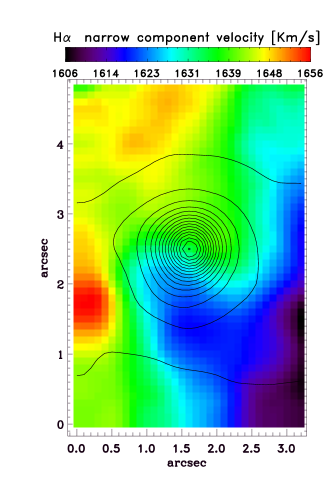
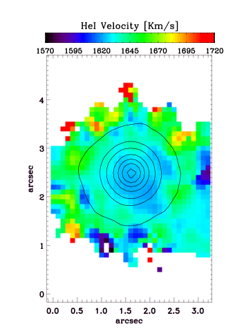
Figure 4: Radial velocity maps. (Left) Map of the narrow component of the H$\alpha$ line. This map is representative of all other narrow-line maps (e.g., narrow [O iii] $\lambda$5007, [O i] $\lambda$6300, [S ii] $\lambda$6717). (Right) Map of the He i $\lambda$7065 line. This map is representative of other broad-line maps (e.g., [O iii] $\lambda$4363, broad H$\alpha$). Contours are the monochromatic intensity of the corresponding emission-line from decreasing intensity intervals of $2\times 10^{-17}$  erg $\hbox{cm}^{2}$ s^-1in peak intensity for H$\alpha$ and $10^{-18}$  erg $\hbox{cm}^{2}$ s^-1for HeI. Only pixels above 3 $\sigma$ of the noise are shown for HeI. In both panels, north is up and east is to the left.

As discussed above, there are two main regions in Mrk 996 with distinct kinematic properties (see also Thuan et al. 1996; James et al. 2009): the central high-ionization broad-line emission zone and the outer low-ionization narrow-line emission zone. We now present maps of both regions in the strongest emission lines and use them to discuss the kinematics of the broad and narrow components. All maps presented here made extensive use of the QFitsView astronomical package. In particular, the function velmap goes through a datacube and fit a Gaussian to a line. The arguments CENTER and FWHM, provided by the user, are used as initial estimates for the gauss-fit. The task then returns the results of the best fit, primarily the fit line center and fit line FWHM, producing the corresponding radial velocity and velocity dispersion maps.

Figure 4 (left panel) shows the radial velocity maps for the narrow component of the H$\alpha$ line. Velocity maps of other narrow lines such as [O i] $\lambda$6300, [S ii] $\lambda$6717, and narrow [O iii] $\lambda$5007 are similar to the H$\alpha$ narrow-component map, and are not shown. All maps are consistent with a systemic velocity of $\sim$ 1640 km s^-1, in agreement with the velocities of the narrow lines in the integrated spectrum (Table 3). Examination of the H$\alpha$ narrow component velocity map reveals a blueshift in the SW direction and a redshift in the NE direction, indicative of an overall rotation pattern. The kinematic pattern changes in the inner 2 ″ where the symmetry axis becomes oriented in the EW direction. Such a twisted velocity map suggests an isotropic gas outflow from the center, superimposed on a rotation pattern of the underlying disc. We also note the presence of a high-velocity feature, perhaps produced by an outflow blob, in the SE direction, at the position $x$= 0$\aas@@fstack{\prime\prime}$2 and $y$= 1$\aas@@fstack{\prime\prime}$8. This high-velocity component is seen only in the direction diametrically opposite to the region of high extinction in the NW discussed below. We will discuss this high-velocity feature further below.

Figure 4 (right panel) shows the radial velocity map for the broad He i $\lambda$7065 line emission in the central region. In contrast to the narrow H$\alpha$ line emission map, it shows no overall rotation pattern. The velocity of the nuclear broad-line emission is blueshifted with respect to that of the narrow component, in agreement with the broad-line velocities in the integrated spectrum (Table 3). There is some indication of slightly higher radial velocities in regions around the nuclear region. This ring-like velocity structure may indicate isotropic motions around the central region. There is, however, one striking exception: the radial velocity map of the [O iii] $\lambda$4363 line does not give a systemic velocity in agreement with the one in the nuclear region for other broad lines. The broad [O iii] $\lambda$4363 line emission is concentrated in the central 2″, and it is clearly blueshifted by $\Delta V\sim 60$ km s^-1 with respect to the systemic velocity. This is seen not only in the velocity map, but also in the integrated spectrum, as discussed in Sect. 3.2. We will discuss the kinematics of [O iii] $\lambda$4363 in greater detail below.

4.2 Velocity dispersion maps

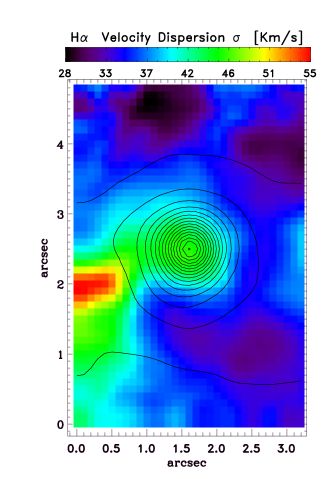
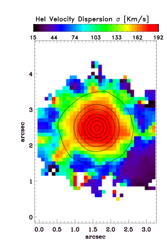
Figure 5: Velocity dispersion maps. (Left) Map of the narrow component of the H$\alpha$ line, representative of all other narrow-line maps (narrow [O iii] $\lambda$5007, [O i] $\lambda$6300, [S ii] $\lambda$6717). (Right) Map of the He i $\lambda$7065 line, representative of all other broad-line maps ([O iii] $\lambda$4363, broad H$\alpha$). The contours and orientation are the same as in Fig. 4.

Figure 5 (left panel) shows the velocity dispersion maps, the left panel for the narrow component of H$\alpha$, and the right panel for the broad He i $\lambda$7065. Again, the narrow H$\alpha$ map is representative of all dispersion maps for the narrow lines, such as narrow [O iii] $\lambda,\lambda$4959, 5007, [O i] $\lambda$6300 and [S ii] $\lambda$6717. These maps show a high central value of $\sigma$ ($FWHM$/2.355) of $\sim$ 45 km s^-1, in agreement with the value given by the integrated spectrum (Table 3). The velocity dispersion then decreases outwards with radius. In the left panel, there is a clear increase in the velocity dispersion towards the outflow blob seen in the radial velocity map, in the SE direction. There are also two low-dispersion regions to the NE and NW, which appear to be related to the high-extinction region seen in the HST color map of Thuan et al. (1996). An additional low-dispersion region is seen in the SW direction. The NE and SW low-dispersion regions are aligned with the overall rotation pattern axis seen in Figure 4, while the outflow blob shows kinematic features about an axis perpendicular to that axis. A patchy velocity dispersion map may indicate the presence of regions with different densities due to the presence of bubbles or shells as seen, for instance, in the study of the internal kinematics of the prototypical HII galaxy II Zw 40 (Bordalo, Plana & Telles 2009).

Figure 5 (right panel) shows the velocity dispersion map for the He i $\lambda$7065 line. As before, this map is similar to those of other broad lines originating from the dense nuclear region. The He i velocity dispersion peaks at the center, with $\sigma\sim 190$ km s^-1 (see also Table 3 for the integrated spectrum), and decreases outwards to values typical of the narrow-line region ($\sigma$ of 50-100 km s^-1). The width of the He i line is similar to that of the broad component of the H$\alpha$ and H$\beta$ lines, and of the [O iii] $\lambda$4363 and [N ii] $\lambda$5755 auroral lines which we discuss next.

4.3 The peculiar kinematics of the [O iii] $\lambda$4363 and [N ii] $\lambda$5755 lines

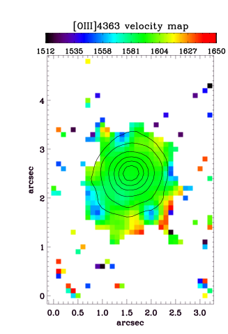
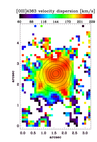
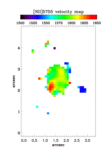
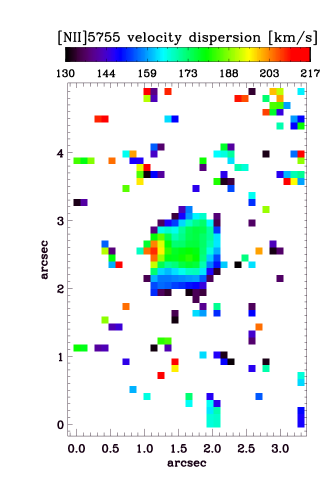
Figure 6: The peculiar kinematics of the [O iii] $\lambda$4363 line (upper panels) and of [N ii]$\lambda$5755 (lower panels). Contours are the monochromatic intensity of the corresponding emission-line from decreasing intensity intervals of $10^{-18}$  erg $\hbox{cm}^{2}$ s^-1in peak intensity. Pixels within the contours are 3 $\sigma$ above noise. North is up and east is left.

.

Figure 6 shows the velocity fields of [O iii] $\lambda$4363 and [N ii] $\lambda$5755. Both lines are totally dominated by the broad emission: the narrow lines, if present, are undetected in the spatially resolved maps. The velocity dispersion of [O iii] $\lambda$4363 is very similar to that of He i $\lambda$7065 (Figure 5), with some structures in the SE-NW direction and an integrated $\sigma\sim 200$ km s^-1. A peak is also seen in the SW direction, but in a region of lower S/N per pixel, so we will not consider it real. The [N ii] $\lambda$5755 line is also broad, though with a somewhat smaller integrated value. The radial velocity maps of these lines have one intriguing peculiarity: both lines are blueshifted with respect to the systemic velocity of the galaxy, by some 60 km s^-1 in the case of [O iii] $\lambda$4363, and by $\sim$20 km s^-1 in the case of [N ii] $\lambda$5755. In addition, [N ii] $\lambda$5755 also shows some structures in the SE-NW in the radial velocity map, suggestive of bipolar outflow motions from the nucleus. The kinematics of the narrow-line region outside the nucleus are, however, not correlated with those of the inner regions, suggesting that the strong motions associated with the broad lines observed are decoupled from motions in the narrow-line region. This interpretation is consistent with the assumption that the outflow motions originate from WR stars in the nuclear region, as is also implied from the flux and velocity maps of the WR blue and red bumps observed in the original data cube. This is also in agreement with the interpretation drawn in Sect. 3.2 for the different systems of emission lines seen in the integrated spectrum.

5 Matching the spatially resolved kinematics with the two-density model

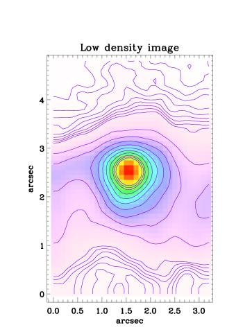
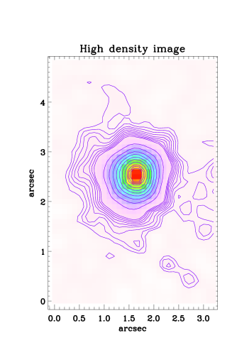
Figure 7: Maps of low (left) and high (right) electron density emission. The orientation is the same as in Fig. 4.

The [S ii] $\lambda$6717/$\lambda$6731 ratio has been widely used in aperture spectroscopy to derive the electron density in H ii regions. The disadvantage is that it only gives an average value of the physical conditions in the region, masking any electron density variation or gradient or any nonuniformity and inhomogeneity in the ionization structure. That the density structure in Mrk 996 is not uniform has been discussed by Thuan et al. (1996), Thuan et al. (2008), and James et al. (2009). Thuan et al. (1996, 2008) had to invoke a CLOUDY model with two zones of different electron densities to account for the integrated optical, near-, and mid-infrared spectra of Mrk 996.

Here, we use a method for mapping low- and high-density clouds in astrophysical nebulae recently devised by Steiner et al. (2009a). This method aims to distinguish regions of low electron densities from those of high electron densities by using individual forbidden line emission images, as opposed to their ratio which may often have low S/N in the outer regions and give untrustworthy results. We will apply this method to the [S ii] $\lambda$6717 and [S ii] $\lambda$6731 emission line images of Mrk 996 to test the hypothesis of a two-density model for the galaxy. These two images are transformed into new images of low- ($I_{ij}(ld)$) and high- ($I_{ij}(hd)$) density emission by applying the Steiner et al. (2009a) formula

$$\left|\begin{array}[]{c}I_{ij}(ld)\\ I_{ij}(hd)\end{array}\right|=\begin{array}[]{c}\underline{\leavevmode\nobreak\ \leavevmode\nobreak\ \leavevmode\nobreak\ \leavevmode\nobreak\ \leavevmode\nobreak\ 1\leavevmode\nobreak\ \leavevmode\nobreak\ \leavevmode\nobreak\ \leavevmode\nobreak\ \leavevmode\nobreak\ }\\ R_{ld}-R_{hd}\end{array}\times\left|\begin{array}[]{cc}1&-R_{hd}\\ -1&R_{ld}\end{array}\right|\times\left|\begin{array}[]{c}I_{ij}(\lambda_{ld})\\ I_{ij}(\lambda_{hd})\end{array}\right|,$$

where $I_{ij}(\lambda_{ld})$ is the [S ii]$\lambda$6717 image, $I_{ij}(\lambda_{hd})$ is the [S ii]$\lambda$6731 image, $R_{ld}$ is the low-density limit ratio of [S ii] $\lambda$6717/$\lambda$6731, and $R_{hd}$ is its high-density limit ratio. From Table 1 in Steiner et al. (2009a), we find $R_{ld}=1.44$ and $R_{hd}=0.44$, corresponding to number densities of 81 cm ^-3 and 5900 cm ^-3, respectively. The latter value should be considered an upper limit to the number density of the gas to which the [S ii] diagnostics can be applied since the critical densities for collisional deexcitation for [S ii] $\lambda$6717 and $\lambda$6731 are 1400 and 3600 cm^-3, respectively (Table 3).

We can apply this method to our integral field observations to assess density variations along the line of sight to the central region of Mrk 996. Figure 7 (left panel) shows the low-density image ($I_{ij}(ld)$) and the right panel shows the high-density image $I_{ij}(hd)$. If the [S ii] emission came only from low-density clouds, all emission would be seen in the left panel only, and none would be seen in the right one. We see clearly that, in Mrk 996, we do have emission along the line of sight from a low-density cloud (left panel) which covers the whole field and emits more in the EW direction. The high-density image (right panel) shows emission concentrated only in the nuclear region. This technique shows clearly that a single low-density regime is ruled out and that an additional regime of high density must be present. These clouds in the nuclear region are probably associated with the broad-line emission shown by some ionic species (e.g., Fig. 4b) and with the WR stars discussed below (see Fig. 14). By performing surface photometry on the high-density image $I_{ij}(hd)$, we derive the diameter of the high-density region to be $\sim$ 1$\aas@@fstack{\prime\prime}$6 or $\sim$ 160 pc, about the size of the inner spiral structure discussed by Thuan et al. (1996) and James et al. (2009). This size coincides with our chosen aperture for the integrated nuclear spectrum shown in Fig. 2.

6 PCA tomography

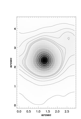
Figure 8: Tomogram (left) and eingeinvector (E₁) in red cube (5700-7200Å). (bottom right) the spectrum from the original data cube; (upper right) the extracted spectrum from the reconstructed data cube, using the PCA tomography results (eigenvector 1 and tomogram 1) (see Steiner et al. 2009b).

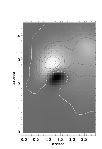
Figure 9: Tomogram (left) and eingeinvector (E₂) in red cube 5700-7200Å  (right). The eigenvector shown in the lower-right panel is a zoom in a shorter wavelength range for a better visualization of the features of interest.

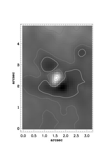
Figure 10: Tomogram (left) and eingeinvector (E₃) in blue cube 4300-5100Å  (right). The eigenvector shown in the lower-right panel is a zoom in a shorter wavelength range for a better visualization of the features of interest.

To fully exploit the wealth and complexity of the information that integral field spectroscopic (IFS) data provide, we need analysis techniques that are more sophisticated than those commonly used in one-dimensional long-slit spectroscopy. However, this new methodology is still scarce, and most IFS studies simply reduce the data cube to one-dimensional spectra and two-dimensional maps, so that the usual well-known spectroscopy and imaging techniques can be applied to analyze the data. Here, we use a technique that has been introduced recently to extract spatial and spectral information from data cubes in a statistical manner, so that it can be used to derive physical information. This technique is called principal component analysis tomography. It combines the statistical PCA analysis, widely used in astronomy, with tomography which is also used in astronomy and other sciences to represent certain types of information derived from imaging techniques. A short presentation of the technique can be found in Steiner et al. (2010).

What PCA tomography basically does is to extract hidden information by transforming a large set of correlated data, in our case the wavelength pixels, into a new set of uncorrelated variables, ordered by their eigenvalues. Each new component, or eigenvector, carries the combined information of the original data, ordered by their significance as measured by their relative variance. The new coordinates can then be represented by their eigenvector and their respective projection called a tomogram. The combined analysis of the eigenvectors and tomograms allows for interpretations of physical phenomena that may not be directly seen in an usual spectrum or image.

Hair et al. (1998) devised a so-called scree test, which was used by Steiner et al. (2009b), and it allows the assessment of the most interesting eigenvectors and tomograms, those that contain most of the relevant information from the data. This test applied to our PCA results shows that the first five eigenvectors and tomograms are sufficient to reconstruct the data cube with the most significant information on the uncorrelated physical properties of the original data.

Table 4: PCA Eigenvalues (blue and red cubes)

Eigenvector	Eigenvalues	Eigenvalues
Ek	Variance (%)	Variance (%)
	5700-7200Å	4300-5100Å
E1	98.15	97.51
E2	1.027	1.552
E3	0.5372	0.2891
E4	0.06388	0.172
E5	0.04478	0.06334
E6	0.0148	0.05601
E7	0.01219	0.0308
E8	0.01171	0.01628
E9	0.008297	0.01367
E10	0.005329	0.01098

Table 4 presents the PCA results from the analysis of the GMOS/IFU data cubes for the red and blue gratings. Column 1 shows the eigenvalue numbers and Cols. 2 and 3 show the resulting variances for the first 10 principal components in the cases of the red and blue gratings, respectively. From these, one can see that the first four principal components carry 99.5% of all uncorrelated information contained in the data.

The first eigenvector in the red cube, which accounts for 98.15% of the data cube variance, is shown in Figure 8. We note that the reconstructed data cube, using only the first principal component (Eigenvector 1 and Tomogram 1), is able to reproduce the original integrated spectrum. The upper-right panel in Fig. 8 shows the representative integrated spectrum obtained by using a reconstructed data cube with only the first eigenvector. This spectrum is identical to the one extracted from the original data cube. The added contribution of eigenvectors 2-5 accounts for only $\leq$ 2% of the variance in the data cube. With the simultaneous analysis of tomogram 1 and the corresponding eigenvector 1, we can reproduce most of the information that can be obtained from a direct broadband image and from an integrated spectrum of the corresponding field of view. This shows the great redundancy of this type of data, allowing for discriminating non-redundant information. The power of this technique lies in the fact that by removing the effects of the strongest correlations, one can look for the less significant ones.

Eigenvector 2 still contributes significantly ($>$1%) and its tomogram reveals distinct bipolar motions originating from the nucleus (Fig. 9). In this case, the y-axis does not represent flux, and the eigenvector is not a spectrum. The point to note is that the eigenvectors are not spectra but vectors of correlations. Here, the anti-correlations (up and down spikes) are seen in the narrow lines only. This means that this particular phenomenon is affecting only the narrow lines. In addition, the feature shows an anti-behavior of the blue side vs. the red side of the lines which leads us to interpret that we are seeing motions in the narrow lines only (e.g., [S ii] 6717,6730). The respective tomogram in Figure 9 (left) shows higher order kinematics of the narrow line. This feature cannot be seen in a classical way as if it were in a direct spectrum, but rather as a residual hidden phenomenon carrying only 1% of the variance. One may interpret this anti-correlation as representing the second-order rotation of a low-density cloud system in the circumnuclear region. Therefore, the broad lines observed in Mrk 996 are probably not due to a turbulent mixing layer, as postulated by James et al. (2009). The present interpretation is more consistent with the hypothesis that the broad lines originate from stellar wind outflows from WR stars in the nuclear region, as implied from the flux and velocity maps of the WR blue and red bumps observed in the original data cube, convoluted with some rotation of the low-density gas within this unresolved inner region. Our analysis is based on two independent data sets, the blue and the red cubes. The features observed in the eigenvectors and tomograms of both data sets are all very similar, which lends credibility to our interpretations.

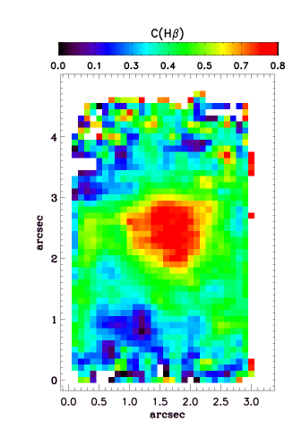
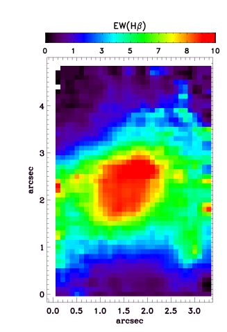
Figure 11: (Left) Logarithmic extinction coefficient map derived from the Balmer decrement using integrated line profiles (broad + narrow components). Pixels with high noise at the border were masked out. (Right) H$\beta$ equivalent width map (per pixel in Å). The orientation is the same as in Fig. 4.

Eigenvector 3 contributes about 0.5% of the variance of the blue cube. It also reveals a strong feature from its tomogram (Figure 10, left) which seems to indicate a distinct intensity contribution from the narrow lines originating in the region surrounding the nucleus, which is different than that of the broad lines. It is noteworthy that the highest intensity features correspond to the positive correlation shown in the broad lines. These features are mapped as white and black pixels in the tomogram and coincide with the broad-line and high-density emission region as extensively discussed above. The lower intensity negative correlation corresponds to the narrow-line and low-density emission region as mapped with gray pixels in the tomogram, but the most important feature can be seen in the zoomed eigenvector (Figure 10, bottom right) where a narrow contribution to the [O iii]$\lambda$ 4363 line is unequivocally detected. This narrow component is not directly seen in the integrated spectrum, but it shows up in this third eigenvector as a dip feature. It is a fundamental finding for our purpose and validates our effort to extract a spatially resolved integrated spectrum which excludes the nuclear region. This will allow for the direct and precise determination of chemical abundances in Mrk 996 (see below) without having to resort to modeling as Thuan et al. (1996) did. We note that this direct and precise mapping of the narrow component of the [O iii]$\lambda$ 4363 line could not be achieved with the data of James et al. (2009) because the narrow component was not detected in their observations with a lower signal-to-noise ratio.

Eigenvector 4 (not shown) contributes only $\sim$0.1% of the variance, but it contains a visible feature in the NW direction. This feature is not related to the emission lines but to the continuum. It may represent, in a statistical way, the effect of dust obscuration. Extinction in that direction has been noted above from analysis of the original cube, through mapping of the Balmer decrement. It can also be seen from the HST broadband images (Thuan et al. 1996). Eigenvector 5 (not shown) contributes less than 0.1% of the variance, and it carries virtually no additional information on uncorrelated physical properties. The higher order eigenvectors and tomograms become more difficult to interpret and/or reach noise features or fingerprints that may not be real, but are instead associated with detector defects and other artificial features. We note that the PCA tomography technique can be used to eliminate higher order noise of the original data by the suppression of detector defects (fingerprints), noise, and by the reconstruction of the data cube accounting only for the first meaningful eigenvectors. A lengthier discussion of this topic is beyond the scope of the present paper. Admittedly, the interpretation of the PCA tomography is not straightforward, but it becomes robust when combined with all other information available. The use of PCA tomography for analyses similar to the one presented here can be found in more recent works, such as Steiner et al. (2013), Sanmartim et al. (2013), Riffel et al. (2011), Ricci et al. (2011), and Schnorr Müller et al. (2011).

7 Mapping the physical conditions

7.1 Extinction and H$\beta$ equivalent width maps

The extinction map in Figure 11 (left panel) was derived by the ratio of the broad+narrow components of the H$\alpha$ and H$\beta$ emission lines. It shows that the nuclear region of Mrk 996 has a higher extinction ($C$(H$\beta$) $\sim$ 0.7). It is surrounded by a region of lower extinction, with $C$(H$\beta$) decreasing to zero. Some higher extinction extension towards the NW and E directions are seen in this map. The central part of the high $C$(H$\beta$) region coincides with the broad-line high-density region. As emphasized in Sect. 3.3, the H$\alpha$/H$\beta$ ratio in this region cannot be used for extinction measurements, as collisional excitation of hydrogen in the nuclear region may make the Balmer decrement and the derived extinction value there artificially high (Fig. 11, left). The regions outside the nucleus show $C$(H$\beta$) $\sim$ 0.4, in good agreement with the extinction derived from the integrated spectrum outside the nucleus (see below Table 5). Figure 11 (right panel) shows the map of H$\beta$ equivalent widths [EW(H$\beta$)] per pixel. It appears that the highest values are not centered on the nucleus but rather in the NW direction, or in a circular ring just outside the nuclear region. Since the broad component in H$\beta$ is primarily seen in the central part of the galaxy, the integrated EW(H$\beta$) per pixel drops steeply outwards.

7.2 Maps of line ratios sensitive to electron temperature and density

Figure 12 shows the spatial distribution of the [S ii] $\lambda$6717/[S ii] $\lambda$6731 ratio. Low values (corresponding to the high-density regime, $N_{e}\geq 10^{3}$ cm^-3) of this ratio are seen in the central region, with a gradient towards higher values (corresponding to the low-density regime, $N_{e}\leq 10^{2}$ cm^-3) outside the nucleus, in good agreement with Figure 7.

The ratio of the [O iii] emission from an upper level (the auroral line, $\lambda$4363) relative to that from lower levels (the nebular lines, $\lambda\lambda 4959,5007$) is known to be highly temperature sensitive. For the low-density region, the electron temperatures with the low-density approximation, typical of the warm ionized gas in H ii regions, range from 10000-20000 K. However, as mentioned above, the very high flux ratios we find in the central regions is due to the very high density and thus the low-density approximation for temperature determination is no longer applicable. Mapping this ratio over the whole extent of our FOV is more difficult in our case, since in the nuclear region the narrow line is unresolved and in the outer region the broad line is not present. The integrated (broad+narrow) line ratio would yield an unphysical result since, as mentioned in § 3.2, the different line systems originate from regions with completely different physical conditions. We have only used this ratio in the integrated spectrum of the region surrounding the nucleus (outer spectrum) in order to derive the chemical abundances directly, as described below.

7.3 Diagnostic diagrams

Figure 13 shows maps of some narrow emission-line ratios of interest such as log([O iii] $\lambda$5007/H$\beta$) (left panel), log([N ii] $\lambda$6584/H$\alpha$) (middle panel), and log([S ii] $\lambda$6717,6731/H$\alpha$) (right panel). These ratios are often used in a diagnostic diagram, known as the Baldwin et al. (1981) (BPT) diagram, to identify the source of excitation in narrow emission-line galaxies. We have used the mapping of these ratios to assess the source of ionization in individual patches of the interstellar medium (ISM) in Mrk 996 (see also Lagos et al. 2009, 2012). Examination of the spatial distribution of these diagnostic ratios shows that regions of intense emission of high-ionization species ([O iii]) are coincident with those of weak emission of low-ionization species ([N ii], [S ii]), implying a single source of ionization, namely the UV radiation from massive stars. The conclusion is the same if we plot the BPT diagram pixel by pixel (not shown here) instead of using maps of individual ratios. Similar results and conclusions were obtained by James et al. (2009). All points fall in the locus predicted by models of photo-ionization by massive stars (e.g., Osterbrock & Ferland 2006). However, it has been shown by Stasińska et al. (2006) and Groves et al. (2006) that an AGN hosted by a low-metallicity galaxy would not be easily distinguished in such a diagram, even if the active nucleus contributed significantly to the emission lines. In fact, the presence of the [O iv] $\lambda$25.89 $\mu$m in the MIR spectrum of Mrk 996 (Thuan et al. 2008) implies the presence of harder ionizing radiation than the stellar one. Thuan et al. (2008) analyzed several possible sources of this radiation, including the presence of an AGN, and concluded that the most probable source is photo-ionization by fast shocks plowing through a dense ISM. In a Chandra X-ray study of Mrk 996, Georgakakis et al. (2011) did not find evidence for an AGN and also attributed the [O iv] $\lambda$25.89 $\mu$m emission to shocks associated with supernova explosions and stellar winds.

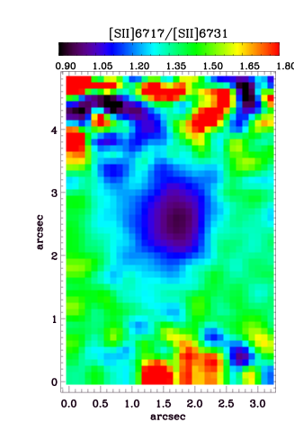
Figure 12: Map of the [S ii] $\lambda$6717/[S ii] $\lambda$6731 ratio. The orientation is the same as in Fig. 4.

7.4 Wolf-Rayet star emission

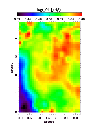
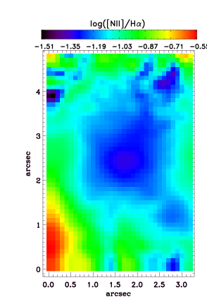
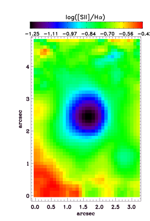
Figure 13: Excitation maps: BPT diagram of narrow emission line ratios. (Left) log([O iii] $\lambda$5007/H$\beta$). (Middle) log([N ii] $\lambda$6584/H$\alpha$. (Right) log([S ii] $\lambda$6717,6731/H$\alpha$. The orientation is the same as in Fig. 4.

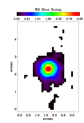
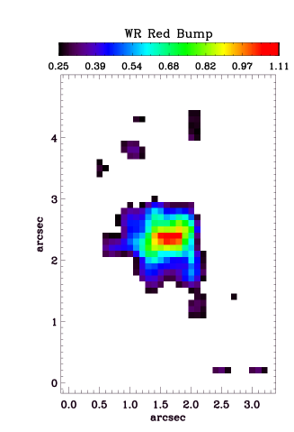
Figure 14: Maps of Wolf-Rayet spectral features. (Left) Blue bump (without the [Fe iii] emission). (Right) Red bump. The fluxes in the bumps are given in units of 10^-16 erg s^-1 cm^-2. The orientation is the same as in Fig. 4.

Thuan et al. (1996) and James et al. (2009) found a large population of Wolf-Rayet stars in the central part of Mrk 996. Figure 14 shows maps of the spectral features associated with this Wolf-Rayet stellar population. These maps were created by summing the fluxes within the wavelength range of interest, and subtracting the adjacent continuum. We have excluded from it the narrow [Fe iii] $\lambda$4658 line.

The left panel shows the map of the blue bump which includes the [N iii] $\lambda$4640 and He ii $\lambda$4686 emission features. The right panel shows the map of the red bump due to the weaker C iv $\lambda$5808 emission. The blue bump emission appears to be more extended spatially than the red bump emission, though this is just a consequence of the lower S/N in the red bump feature. The maps show that the blue and red bumps are coincident spatially and that their spatial distributions are identical to those of the broad He i and H$\alpha$ emissions. This implies that the WR stars are located and concentrated solely in the nuclear region of Mrk 996.

The total observed (uncorrected for extinction) flux of the blue bump is $3.87\times 10^{-14}$ erg s^-1 cm^-2, while that of the red bump is $1.14\times 10^{-14}$ erg s^-1 cm^-2. These fluxes derived directly from the maps are a factor of $\sim$ 2 larger than those derived from the integrated spectrum as described in § 3.4. The origin of this discrepancy is probably due to our not performing here a proper deblending of the nebular lines (i.e., [Fe iii] $\lambda$4658, [Fe iii] $\lambda$4702, and He i 4713). Thus, a more detailed quantitative comparison with the integrated spectrum is not warranted. With the maps, we wish only to show the region where the WR emission originates.

7.5 Physical conditions and oxygen and nitrogen abundances of the outer narrow-line region

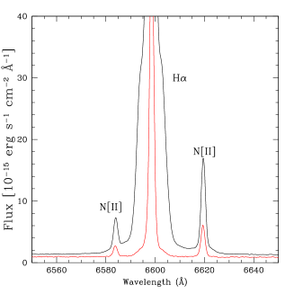
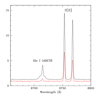
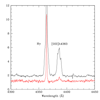
Figure 15: Spatially narrow-line region spectrum (lower red spectrum) displayed with the integrated spectrum of the nuclear region (upper black spectrum).

The integrated nucleus spectrum of Figure 2 clearly shows the presence of blended broad and narrow lines. Table 3 presents the emission line fluxes of both broad and narrow components derived from this integrated nucleus spectrum (obtained through a $\sim$1$\aas@@fstack{\prime\prime}$6 aperture) after line deblending. As discussed in Sect. 5, we have been able to separate spatially the nuclear broad-line region from the surrounding narrow-line region by using the electron density diagnostic map (Figure 7). The broad-line region, where the He i, [O iii] $\lambda$4363, and [N ii] $\lambda$5755 lines, and the Wolf-Rayet blue and red bumps originate, coincides with the high-density region, with a diameter of $\sim$ 1$\aas@@fstack{\prime\prime}$6, in the electron density diagnostic maps. The diameter of $\sim$160pc of the nuclear broad-line and high electron density region is consistent with the size derived by Thuan et al. (1996) by CLOUDY photo-ionization modeling of the nuclear emission of Mrk 996.

Having spatially resolved the broad-line and high-density region of Mrk 996 by the use of the various diagnostic maps, we can now go one step further: we can exclude the nuclear region and extract an integrated spectrum of the light that comes exclusively from the narrow-line region surrounding the nucleus. Figure 15 shows the outer narrow-line region spectrum in red lines (lower spectrum). For comparison, the integrated spectrum of the nuclear region is shown by a black line (upper spectrum). We emphasize that the narrow lines are not derived from a decomposition of the blended lines, but they are measured from the actual integrated spectrum in the region outside the nucleus. The three panels in Fig. 15 show several lines of interest, and are labeled [O iii] $\lambda$4363, H$\alpha$, and He i $\lambda$6678. It can be seen that the narrow component of [O iii]$\lambda$4363 in the outer region is very weak, but clearly detected at a 7 $\sigma$ level. This weak line is swamped by the broad component in the nuclear region and not detectable at lower S/N observations. One can also see that the narrow line of [O iii] $\lambda$4363 in the outer region, as opposed to the broad line of [O iii] $\lambda$4363 in the integrated nucleus region, is not blueshifted. It falls in the same systemic recession velocity derived from the narrow components of the lines in the integrated nucleus region. The existence of this narrow component originating from the low-density region has also been demonstrated by a completely independent technique, that of PCA tomography, as discussed in Sect. 6. The [N ii] and [S ii] lines show a narrow component everywhere, independent of the density. We note the high value of the [S ii] $\lambda$6717 / $\lambda$6731 ratio in the narrow-line region, indicative of a low electron density.

Table 5: Emission line parameters derived from the outer spectrum within a 2.7 x 4.4″excluding the inner circle with 1.3″radius

Ion	$\lambda_{0}$	F($\lambda$)/F(H$\beta$)	$v(rad)$	$FWHM$
$[$O ii$]$	3726.03	88.84$\pm$ 20.8	1628	99$\pm$3
$[$O ii$]$	3728.82	146.52$\pm$ 26.1	1625	131$\pm$3
$[$Ne iii$]$	3868.75	40.53$\pm$ 16.6	1627	156$\pm$4
H8+He i	3889.05	25.09$\pm$ 15.7	1614	114$\pm$3
$[$S ii$]$	4068.60	46.87$\pm$ 7.05	1603	78$\pm$2
H$\delta$	4101.74	23.50$\pm$ 5.20	1623	98$\pm$3
H$\gamma$	4340.47	42.01$\pm$ 3.71	1620	101$\pm$3
$[$O iii$]$	4363.21	3.34$\pm$ 2.01	1627	143$\pm$4
He i	4471.48	3.87$\pm$ 2.04	1615	114$\pm$3
H$\beta$	4861.33	100.00$\pm$ 2.93	1626	123$\pm$3
$[$O iii$]$	4958.91	96.60$\pm$ 2.72	1627	121$\pm$3
$[$O iii$]$	5006.85	276.46$\pm$ 3.84	1626	120$\pm$3
He i	5875.67	13.24$\pm$ 1.52	1633	109$\pm$3
$[$O i$]$	6300.30	4.85$\pm$ 1.17	1631	99$\pm$3
$[$S iii$]$	6312.10	2.01$\pm$ 1.15	1633	110$\pm$3
$[$O i$]$	6363.78	1.64$\pm$ 1.09	1635	100$\pm$3
$[$N ii$]$	6548.03	10.80$\pm$ 0.98	1641	93$\pm$2
H$\alpha$	6562.82	366.07$\pm$ 3.71	1634	91$\pm$2
$[$N ii$]$	6583.41	29.83$\pm$ 1.75	1639	90$\pm$2
He i	6678.15	3.95$\pm$ 1.07	1637	109$\pm$3
$[$S ii$]$	6716.47	33.34$\pm$ 1.47	1638	85$\pm$2
$[$S ii$]$	6730.85	24.84$\pm$ 1.82	1638	88$\pm$2
He i	7065.28	1.91$\pm$ 1.36	1635	83$\pm$2
$[$Ar iii$]$	7135.78	9.90$\pm$ 1.42	1637	84$\pm$2

$F_{nar}$(H$\beta$)=(35.60$\pm$2.10)$\times$10^-15 erg s^-1 cm^-2
$c($H$\beta_{narrow})=0.31$

Figure 16: Comparison of the measured line fluxes in the integrated spectrum of the outer region outside the nucleus (Table 5) with the fluxes measured in the narrow components of the integrated spectrum of the nucleus of Mrk 996 (Table 3).

We can now use the measured line fluxes, shown in Table 5 from the spatially separated narrow-line region spectrum (red-line lower spectra in Figure 15) to derive the physical conditions and element abundances in the low-density outer region. As expected, the line fluxes measured outside the nucleus are in good agreement with the measured fluxes of the narrow components of the integrated spectrum in the nuclear region, as shown in Figure 16, corroborating our statement that this zone of low density is on the line of sight of the inner broad-line dense nucleus. By scaling the intensity of the [O iii] $\lambda$4363 in the outer region with the narrow H$\beta$ flux ratio of the outer region to the nuclear region, we estimate that the narrow component of the [O iii] $\lambda$4363 in the nuclear region must be $\sim$ 4 fainter than the integrated line, which explains the difficulty in detecting this line directly in the integrated nuclear spectrum.

7.5.1 Oxygen abundances

We make use of the nebular package available in the stsdas external package under IRAF to derive abundances. The tasks in this package are based on a five-level atom model developed by De Robertis et al. (1987). The detection of [O iii] $\lambda$4363 allows a direct determination of the electron temperature $T_{e}$(O⁺⁺)=$1.29\times 10^{4}$K, while the ratio of the [S ii] lines permits us to determine a low electron density in this narrow-line region of $N_{e}\sim$71 cm^-3. We obtain 12+log(O/H)=7.94$\pm 0.30$ using $C$(H$\beta$)=0.31, that is, Z_⊙/6 by adopting the solar calibration of Asplund et al. (2009). The same result 12+log(O/H)=7.88$\pm 0.36$ is obtained using the T_e direct method with the prescriptions of Pagel et al. (1992), Izotov et al. (1994), and Thuan et al. (1995).

This oxygen abundance is in agreement with the value of Thuan et al. (1996) who derived 12+log(O/H)=8.0 with a CLOUDY two-zone model of Mrk 996. It is, however, considerably less (by a factor of at least 3) than the lower limit of 12+log(O/H) $\sim$ 8.37 obtained by James et al. (2009) for the broad-line region, based on an assumed electron temperature of 10,000 K. Our value of the oxygen abundance is more reliable since the [O iii] $\lambda$4363 line intensity, and hence the electron temperature, was determined directly in the low-density region outside the nucleus.

7.5.2 Nitrogen abundances

The derived nitrogen abundance for the low-density region is log(N/O)=$-$1.53$\pm$0.15, in good agreement with the value of $-$1.43 obtained by James et al. (2009). It is typical of values derived for BCDs (Izotov et al. 2006).

However, the nuclear region is nitrogen enhanced by a factor of $\sim$ 20, with log(N/O)=$-$0.15$\pm 0.1$. In this case, we assumed a two-density model in nebular, with $N_{e}$(low)=450 cm^-3, $N_{e}$(high)=$10^{6}$ cm^-3, $T_{e}$(low)=$10^{4}$K and $T_{e}$(high)=$4\times 10^{4}$K. $T_{e}$(high) is derived from the extinction corrected ratio of [OIII] broad-line fluxes assuming $N_{e}$(high). Our high N/O in the broad-line region is in agreement with that obtained by Thuan et al. (1996) from CLOUDY modeling (model 2), and with the value of $-$0.13 obtained by James et al. (2009). This nitrogen enhancement is probably due to local pollution from WR stars. Similar cases for a nitrogen enhancement have been observed, for example, in the central region of the nearby dwarf starburst galaxy NGC 5253 by Westmoquette et al. (2013), and for the very metal-deficient (12+ log (O/H)=7.64) luminous (MB= -18.1m) blue compact galaxy (BCG) HS 0837+4717 by Pustilnik et al. (2004). Brinchmann et al. (2008), in turn, have noted an elevated N/O for galaxies with Wolf-Rayet features in their optical spectrum from SDSS survey. López-Sánchez & Esteban (2010) have also detected a high N/O ratio in objects showing strong WR features (HCG 31 AC, UM 420, IRAS 0828+2816, III Zw 107, ESO 566-8, and NGC 5253). They claim that the ejecta of the WR stars may be the origin of the N enrichment in these galaxies. However, as pointed out by Izotov et al. (2006), this high N/O cannot be caused by WR nitrogen-enriched ejecta with a number density $N_{e}$ similar to that of the ambient gas, but only by considerably denser ejecta since the emissivity of the [N ii] lines is proportional to $N_{e}^{2}$.

8 Summary and conclusions

The galaxy Mrk 996 is an extraordinary blue compact dwarf galaxy with a dense unresolved nucleus ($<160$ pc) and a central density of $\sim$10⁶ cm^-3. The dense nucleus is surrounded by a lower density star-forming region, with a density of $\sim$10² cm^-3. We present here integral field spectroscopy obtained with GEMINI-SOUTH/GMOS/IFU which allows us to study in 2D the physical conditions, ionization structures, and kinematic properties of these two regions, as well as their relationship.

We have made an extensive comparison with the results of the previous similar IFU work by James et al. (2009) on Mrk 996. Our results fully agree with theirs on the spatial variation of the physical properties and detected internal structures of Mrk 996. However, our quantitative results differ somewhat in the number of massive stars present in the star forming nucleus, and in the determination of the chemical abundances. The first disagreement may be partly due to absolute calibration differences. Their fluxes are a factor of $\sim$ 5 brighter than our simulated VIMOS aperture. We believe our reduction and calibration procedures to be correct as they have been double-checked independently by us using different standard stars. The red cube and blue data cubes were derived from observations of different nights and the calibrations agreed, without the need for averaging the data. Other external checks have also shown consistency. More importantly, we have made a more precise determination of oxygen abundance in the low-density gas by directly detecting the narrow line of [OIII]$\lambda$4363 outside the nucleus. This detection was confirmed, independently, by the use of a new innovative method of data cube analysis.

We have thus obtained the following results:

1) The integrated spectrum shows four kinematically distinct systems of emission lines, with line-widths decreasing outwards from the center. The first system shows both broad and narrow lines, originating from the nuclear region. The broad component is probably associated with the circumnuclear envelopes around WR stars, while the narrow component is probably related to the circumnuclear envelopes around O stars. The second system comes from the innermost and densest part of the star-forming region. It consists of the peculiar emission of the [O iii]$\lambda$4363 line which is broad ($\sigma\sim 200$  $\hbox{km}\thinspace\hbox{s}^{-1}$) and blueshifted by 60  $\hbox{km}\thinspace\hbox{s}^{-1}$ relative to the narrow H$\beta$ line. The third system consists of the permitted hydrogen and helium lines, and of the auroral [N ii] line. These also show large widths, similar to those in the second system, but are less blueshifted ($\sim 20$  $\hbox{km}\thinspace\hbox{s}^{-1}$). They are likely to originate in regions farther away from the center than the second line system. The fourth system consists only of narrow lines of hydrogen, helium, doubly ionized ions, and of forbidden lines of neutral and singly ionized species. These all have the same radial velocities as the H$\beta$ emission line.

2) Most of the observed physical conditions and kinematics of the nucleus of Mrk 996 appear to be related to the presence of a Wolf-Rayet stellar population, as inferred by the presence of the blue and red bump spectral features. We estimate, from the integrated spectrum as well as from the spatially resolved maps of these features, that the nuclear region of Mrk 996 contains $\sim$ 473 WNL and $\sim$ 98 WCE stars, with $N$(WR)/$N$/(O+WR)=0.19, at the high end for WR galaxies.

3) The monochromatic emission maps and the line ratio, velocity, and dispersion maps of the nuclear region suggest an isotropic ionized gas outflow from the center ($<$160 pc), superposed on an underlying rotation pattern. This outflow is probably associated with the ejecta from the WR stellar population. The narrow ($\sigma\sim 45$ $\hbox{km}\thinspace\hbox{s}^{-1}$) and broad ($\sigma\sim 200$ $\hbox{km}\thinspace\hbox{s}^{-1}$) lines from the nucleus are supersonic. The [O iii]$\lambda$ 4363 and [N ii]$\lambda$ 5755 lines show peculiar kinematics, suggestive of outflow motions from the nucleus, or multiplicity due to a patchy ISM.

4) We have also performed a PCA tomography analysis that corroborates, in a completely independent manner, the kinematic picture outlined above for Mrk 996: an outflow from the inner region, associated with winds from WR stars, superposed on an underlying rotation pattern, affecting the motions of low-density clouds. This recently developed statistical method for handling data cubes has also resulted in the independent detection of the narrow component of the [O iii]$\lambda$ 4363 line, not seen previously in integrated spectra. This detection allows a reliable and direct measurement of the chemical abundances in the region outside the nucleus.

5) We obtain an oxygen abundance 12+log(O/H)=7.90$\pm 0.30$ ($\sim$ 0.2 $Z_{\odot}$) for the low-density narrow-line region around the nucleus, in agreement with the abundance derived by Thuan et al. (1996), but considerably less than the lower limit of 12+logO/H=8.37 derived by James et al. (2009) for the broad-line region, based on an assumed electron temperature. The N/O ratio in the low-density region is typical of BCDs. However, as discussed by previous investigators, there is a nitrogen enhancement by a factor of $\sim$ 20 in the nuclear region, probably due to nitrogen-enriched WR ejecta, but also to enhanced nitrogen line emission in a high-density environment. The presence of a large number of WR stars in the nucleus of this dwarf starburst galaxy greatly affecting its local kinematics is somewhat unexpected because of its sub-solar oxygen abundances. If we take the results of stellar population models at face value (see, e.g., Cerviño & Mas-Hesse 1994), this implies that we are witnessing a very short phase of the evolution of the starburst in Mrk 996.

6) Finally, we have used a method recently proposed by Steiner et al. (2009a) to map low- and high-density regions in Mrk 996. By performing surface photometry on the resulting high-density image, we have obtained an upper limit of $\sim$ 1$\aas@@fstack{\prime\prime}$6 ($\sim$ 160 pc) for the diameter of the nuclear region. This region is where the broad lines originate. The emission line ratios in the BPT diagnostic diagram appear to indicate ionization from UV radiation of massive stars alone. The presence of harder ionizing radiation, as implied by the presence of the [O iv] $\lambda$25.9 $\mu$m emission-line in its MIR spectrum (Thuan et al. 2008), is most likely due to fast radiative shocks propagating in a dense interstellar medium. This is in agreement with the Chandra X-ray study of Mrk 996 by Georgakakis et al. (2011) who rule out an AGN, but also favor shocks as the ionization source for the [O iv] $\lambda$25.9 $\mu$m emission. We intend to investigate this issue further with new integral field observations in the near-IR with adaptive optics. This will allow us to set more stringent upper limits to the size of the broad-line emitting region, and also to study additional physical properties of the nebular emission in this wavelength range including possible H₂ emission that probe the warm molecular gas in the shells around the photo-dissociation regions.

The advent of Integral Field Units has allowed spatially resolved spectroscopy, with the simultaneous acquisition of a complete set of spectra covering a spatially resolved field of view. Despite this great instrumental advance, the superior and abundant data that are obtained with IFUs are still mostly analyzed with the traditional techniques of 1D slit spectroscopy. Although these traditional methods are useful for a first look at the data, they do not fully exploit the wealth of information given by integral field spectroscopy. In some cases, they may not even be the proper tools to use, particularly when assumptions on boundaries of regions need to be made, or other structure-dependent physical equilibria need to be assumed. We have attempted to apply a few new techniques to the data in this paper, and they have yielded useful results. More new methodologies for analysis are required, and we will apply them as they are devised.