Approximate Bayesian Probabilistic Data Association Aided Iterative Detection for MIMO Systems Using Arbitrary $M$-ary Modulation

Abstract

In this paper, the issue of designing an iterative detection and decoding (IDD) aided receiver relying on the low-complexity probabilistic data association (PDA) method, is addressed for turbo-coded multiple-input–multiple-output (MIMO) systems using general $M$-ary modulations. We demonstrate that the classic candidate-search aided bit-based extrinsic log-likelihood ratio (LLR) calculation method is not applicable to the family of PDA-based detectors. Additionally, we reveal that in contrast to the interpretation in the existing literature, the output symbol probabilities of existing PDA algorithms are not the true a posteriori probabilities (APPs), but rather the normalized symbol likelihoods. Therefore, the classic relationship, where the extrinsic LLRs are given by subtracting the a priori LLRs from the a posteriori LLRs does not hold for the existing PDA-based detectors. Motivated by these revelations, we conceive a new approximate Bayesian theorem based logarithmic-domain PDA (AB-Log-PDA) method, and unveil the technique of calculating bit-based extrinsic LLRs for the AB-Log-PDA, which facilitates the employment of the AB-Log-PDA in a simplified IDD receiver structure. Additionally, we demonstrate that we may dispense with inner iterations within the AB-Log-PDA in the context of IDD receivers. Our complexity analysis and numerical results recorded for Nakagami-$m$ fading channels demonstrate that the proposed AB-Log-PDA based IDD scheme is capable of achieving a comparable performance to that of the optimal MAP detector based IDD receiver, while imposing a significantly lower computational complexity in the scenarios considered.

I Introduction

When conceiving advanced wireless systems using both multiple-input–multiple-output (MIMO) techniques [1, 2] and near-capacity forward error correction (FEC) codes [3, 4, 5] to simultaneously achieve a high throughput and an infinitesimally low error rate, one of the major challenges is the potentially prohibitive computational complexity at receiver. The iterative detection and decoding (IDD) [6], which was inspired by decoding of concatenated codes [3, 7], is capable of achieving a near-optimum performance at a significantly lower complexity than the maximum-likelihood sequence estimator based optimal joint detector/decoder [8, 9]. Even so, the computational complexity imposed by the IDD might remain the limiting factor in practical applications.

The probabilistic data association (PDA) filtering method was highly successful for target tracking problems [10, 11] in radar systems. In digital communications, it may also be developed to a soft-input–soft-output (SISO) efficient interference-modelling method [12, 13, 14, 15, 16, 17]. The key feature of PDA is the repeated conversion of a multimodal Gaussian mixture probability to a single multivariate Gaussian distribution. Therefore, the accuracy of the Gaussian approximation dominates the attainable performance. In uncoded MIMO systems using quadrature amplitude modulation (QAM), the quality of the Gaussian approximation in PDA may be improved by transforming the symbol-based model into a bit-based model, which in effect increases the length of the effective transmitted signal vector by the number of bits per symbol, and reduces the effective constellation to a binary constellation [16]. With regard to improving the quality of the Gaussian approximation in FEC-coded MIMO systems, we benefit from having an increased exploitable degree of freedom. For example, the soft information gleaned from the output of the FEC decoder tends to be more reliable than the output symbol probabilities of the PDA detector itself. Therefore the FEC decoder’s soft output would facilitate a more accurate modelling of the inter-antenna interference (IAI). The iterative receiver proposed in [18] was essentially a maximum a posteriori (MAP) detection aided IDD scheme, employing the hard-output PDA detector for generating the candidate-search list, hence it did not solve the problem of interest to us.

There are several particular challenges that render the IDD design using PDA less straightforward than it seems to be. Firstly, to the best of our knowledge, all the existing PDA detectors conceived for uncoded systems operate purely in the probability-domain[12, 13, 14, 15, 16, 17], which results in a poor numerical stability in IDD scenarios, hence potentially leading to a degraded performance. Secondly, it is unclear how to produce the correct bit-based extrinsic log-likelihood ratios (LLRs) required by the concatenated outer FEC decoder. Conventionally, the output symbol probabilities of the existing PDA algorithms were interpreted as the a posteriori probabilities (APPs)[12, 13, 14, 15, 16, 17]. Hence, one may assume that a natural way of generating the bit-based extrinsic LLRs is to subtract the bit-based a priori LLRs from the bit-based a posteriori LLRs generated from the output probabilities of the PDA algorithms. However, we will show that this classic relationship no longer holds if we still treat the output symbol probabilities of the existing PDA algorithms as APPs in the context of IDD receivers. Thirdly, the existing PDA algorithms[12, 13, 14, 15, 16, 17] have an inherently self-iterative structure, where the estimated symbol probabilities are delivered to the next inner iteration after the current inner iteration is completed. Then, the question of how to deal with the inner iterations of the existing PDAs in the context of IDD receivers arises.

Against this backdrop, the main contributions of this paper are as follows.

1) We present an analysis of the interference-plus-noise distribution for the MIMO signal model, which sheds light on the fundamental principles of the PDA algorithms from a new perspective.

2) We propose an approximate Bayesian theorem based logarithmic-domain PDA (AB-Log-PDA) MIMO detector for IDD aided MIMO systems employing arbitrary $M$-ary modulations, which has not been reported before. The proposed AB-Log-PDA enjoys better numerical stability and accuracy, hence it is better suited for iterative detection than the existing probability-domain PDA detectors conceived for uncoded systems [12, 13, 14, 15, 16, 17].

3) In contrast to the conventional interpretations of the mathematical properties of the estimated output symbol probabilities of the PDA algorithms, we will demonstrate that these probabilities do not constitute the true symbol APPs, they rather constitute the normalized symbol likelihoods. Owing to this misinterpretation, it is flawed to produce the bit-based extrinsic LLRs from the output symbol probabilities of the PDA algorithms by using the classic relationship, where the extrinsic LLRs are given by subtracting the a priori LLRs from the a posteriori LLRs. We demonstrate furthermore that the classic candidate-search aided bit-based extrinsic LLRs calculation method, which is used for example by the MAP detector and the list sphere decoder, is not applicable to any PDA-based detector. In order to circumvent the above-mentioned problems, we conceive a new technique of producing the bit-based extrinsic LLRs for the proposed AB-Log-PDA, which results in a simplified IDD structure, where the extrinsic LLRs of the AB-Log-PDA are generated by directly transforming the output symbol probabilities into bit-based LLRs, without subtracting the a priori LLRs.

4) We reveal that introducing inner iterations into the AB-Log-PDA actually degrades the achievable performance of the IDD receiver, which is in contrast to the impact of the inner iterations within the FEC-decoder of other types of iterative receivers. The reasons as to why the inner PDA iterations fail to provide BER improvement are investigated and discussed in detail. Notably, we show that the proposed AB-Log-PDA based IDD scheme invoking no inner iterations within the AB-Log-PDA strikes an attractive performance versus complexity tradeoff, which compares favorably to that of the optimal MAP based IDD scheme in both perfect and imperfect channel-estimation scenarios, when communicating over Nakagami-$m$ fading channels. For example, in some scenarios the performance of the proposed AB-Log-PDA based IDD scheme approaches that of the MAP-based IDD scheme within 0.5 dB, while imposing a significantly lower computational complexity.

The remainder of the paper is organized as follows. In Section II, our FEC-coded MIMO system model is introduced, while in Section III, we present our analysis of the interference-plus-noise distribution for our MIMO signal model, which sheds light on the fundamental principles of the PDA from a new perspective. In Section IV, the proposed AB-Log-PDA is presented, which relies on the a priori soft information feedback gleaned from the FEC decoder. Then, in Section V the extrinsic LLR calculation of the AB-Log-PDA is detailed, while our simulation results and discussions are presented in Section VI. Finally, the paper is concluded in Section VII.

II System Model

Figure 1: The FEC-coded MIMO system with a simplified structure for the AB-Log-PDA based IDD receiver, where we have ${\bf{L}}_{E_{2}}={\bf{L}}_{D_{2}}$ rather than the classical ${\bf{L}}_{E_{2}}={\bf{L}}_{D_{2}}-{\bf{L}}_{A_{2}}$. The subscript “1” denotes the processing modules associated with the outer FEC encoder/decoder, and the subscript “2” denotes the processing modules that are connected with the inner space-time mapper/detector. The arrow with dashed line indicates that $\bf{s}$ and ${\bf{L}}_{D}$ are the subvectors of ${\bf{s}}_{2}$ and ${\bf{L}}_{D_{2}}$, respectively.

We consider the FEC-coded MIMO system of Fig. 1. At the transmitter, the $(L_{f}\times 1)$ source-bit frame ${\bf{x}}_{1}$ is firstly encoded by a rate $R<1$ FEC encoder (typically a convolutional code, a turbo code or an LDPC code) into the $(\frac{L_{f}}{R}\times 1)$ coded-bit frame ${\bf{c}}_{1}$. In order to guard against bursty fading, ${\bf{c}}_{1}$ is then passed through a bit-interleaver. Then the $(\frac{L_{f}}{R}\times 1)$ interleaver output bit-frame ${\bf{d}}_{2}$ is mapped to the $(\frac{L_{f}}{RM_{b}}\times 1)$ symbol-frame ${\bf{s}}_{2}$, with each symbol taken from the $M$-ary modulation constellation $\mathcal{A}=\{a_{1},a_{2},\cdots,a_{M}\}$, where $M_{b}=\log_{2}^{M}$ is the number of bits per constellation symbol. Finally, ${\bf{s}}_{2}$ is transmitted in form of the $(N_{t}\times 1)$ vector of symbols $\bf{s}$ by $N_{t}\geq 1$ transmit antennas per channel use.

At the output of the fading channel $\bf{H}$, the received $(N_{r}\times 1)$-element complex-valued baseband signal vector per channel use is represented by

$${\bf{y}=\bf{Hs}+\bf{n}},$$ (1)

where ${\bf{s}}=[s_{1},s_{2},\cdots,s_{N_{t}}]^{T}$ is normalized by the component-wise energy constraint $\mathbb{E}({\left|s_{i}\right|}^{2})=E_{\bf{s}}/N_{t}$ in order to maintain a total transmit power $E_{\bf{s}}$ per channel use; and $\bf{n}$ is the $(N_{r}\times 1)$-element zero-mean complex-valued Gaussian noise vector with a covariance matrix of $2\sigma^{2}{\bf{I}}_{N_{r}}$ where ${\bf{I}}_{N_{r}}$ represents an $(N_{r}\times N_{r})$-element identity matrix; and $\bf{H}$ is an $(N_{r}\times N_{t})$ complex-valued matrix with entries $h_{ji}$ perfectly known to the receiver, $j=1,\cdots,N_{r}$, $i=1,\cdots,N_{t}$. In this paper, we assume that $h_{ji}=r\exp({j\theta})$ is independent and identically distributed (i.i.d), the phase $\theta$ is uniformly distributed and independent of the envelope $r$, while $r$ obeys the Nakagami-$m$ distribution having the probability density function (PDF) of [19]

$$p(r)=\frac{2}{\Gamma(m)}\left(\frac{m}{\Omega}\right)^{m}r^{2m-1}\exp({-mr^{2}/\Omega}),\;r\geq 0,$$ (2)

where $\Gamma(\cdot)$ represents the Gamma function, $\Omega\triangleq\mathbb{E}(r^{2})$, and the Nakagami fading parameter is $m\triangleq{\Omega^{2}}/{\mathbb{E}[(r^{2}-\Omega)^{2}]}$, $m\geq 0.5$. Note that the Nakagami-$m$ fading model captures a wide range of realistic fading environments, encompassing the most frequently used Rayleigh and Rician fading models as special cases. More specifically, the parameter $m$ indicates the severity of the fading. As $m$ becomes smaller, the fading effects become more severe. For example, when $m$ decreases to $0.5$, Eq. (2) approaches the one-sided Gaussian distribution; when $m=1$, Eq. (2) reduces to a Rayleigh PDF, and as $m\rightarrow\infty$, Eq. (2) reduces to a $\delta$-distribution located at $r=1$, which corresponds to imposing no fading on the amplitude of the transmitted signal, but only a “pure random phase” obeying a uniform distribution on the circle of radius $\sqrt{\Omega}$. In addition to its generalized nature, the Nakagami-$m$ fading model was shown to fit the experimental propagation data better than the Rayleigh, Rician and Lognormal distributions [20].

III Interference-Plus-Noise Distribution Analysis

In order to provide more insight on the fundamental principle underlying the PDA method, an interference-plus-noise distribution analysis is carried out in this section.

The received signal model of (1) may be rewritten as

$${\bf{y}}=s_{i}{\bf{h}}_{i}+\underbrace{\sum\limits_{k\neq i}{s_{k}{\bf{h}}_{k}}}_{{\bf{u}}_{i}}+{\bf{n}}\buildrel\Delta\over{=}s_{i}{\bf{h}}_{i}+\underbrace{{\bf{u}}_{i}+\bf{n}}_{{\bf{v}}_{i}},$$ (3)

where ${\bf{h}}_{i}$ denotes the $i$-th column of $\bf{H}$, and $s_{i}$ is the $i$-th symbol of $\bf{s}$, while ${\bf{u}}_{i}$ is the sum of $(N_{t}-1)$ IAI components contaminating the symbol $s_{i}$, $i$, $k=1,2,\cdots,N_{t}$, and ${\bf{v}}_{i}$ is the interference-plus-noise term for $s_{i}$.

Note that if ${\bf{u}}_{i}$ vanishes, Eq. (3) reduces to the classic single-input–multiple-output interference-free broadcast channel having a receive diversity order of $N_{r}$. Similarly, if we know exactly the distribution of ${\bf{u}}_{i}$ or $s_{k}$, this potentially allows us to mitigate the adverse effects of the IAI. However, unfortunately, the distribution of ${\bf{u}}_{i}$ is generally unknown. A notable exception is, when the number of independent IAI components is sufficiently high, ${\bf{u}}_{i}$ approaches a multivariate Gaussian distribution according to the central limit theorem,

On the other hand, we observe that the interference term ${\bf{u}}_{i}$ has a total of $M^{N_{t}-1}$ possible interference patterns. Then, the $n$-th legitimate interference pattern imposed by a given sample of

$$\underline{\bf{s}}_{n}=[\underline{s}_{1,n},\cdots,\underline{s}_{k,n},\cdots,\underline{s}_{N_{t},n}]_{k\neq i}^{T}$$ (4)

is defined as

$$\underline{\bf{u}}_{i,n}\triangleq\sum\limits_{k\neq i}\underline{s}_{k,n}{\bf{h}}_{k},$$ (5)

while the corresponding interference-plus-noise pattern is defined as

$$\underline{\bf{v}}_{i,n}\triangleq\underline{\bf{u}}_{i,n}+\bf{n},$$ (6)

where $\underline{s}_{k,n}=a_{m}\in\mathcal{A}$, $n=1,2,\cdots,M^{N_{t}-1}$. We observe that $\underline{\bf{v}}_{i,n}$ obeys a multivariate Gaussian distribution with a mean of $\sum\limits_{k\neq i}\underline{s}_{k,n}{\bf{h}}_{k}$ and a covariance of $2\sigma^{2}{\bf{I}}_{N_{r}}$ for complex-valued noise, hence the PDF of $\underline{\bf{v}}_{i,n}$ is formulated as

$$f(\underline{\bf{v}}_{i,n})=c\exp\left(-\frac{\lVert\underline{\bf{v}}_{i,n}-\sum\limits_{k\neq i}\underline{s}_{k,n}{\bf{h}}_{k}\rVert^{2}}{2\sigma^{2}}\right),$$ (7)

where

$$c=\frac{1}{\pi^{N_{r}}\det(2\sigma^{2}{\bf{I}})}=\frac{1}{(2\pi\sigma^{2})^{N_{r}}}.$$ (8)

If we assume that the probability of encountering the $n$-th interference pattern caused by $\underline{{\bf{s}}}_{n}$ is $P_{n}$, then upon jointly considering the distribution of $\underline{\bf{s}}_{n}$ and that of $\underline{\bf{v}}_{i,n}$, the distribution of ${\bf{v}}_{i}$ may be characterized by the multimodal Gaussian mixture distribution of

$$p({\bf{v}}_{i})=\sum\limits_{n=1}^{M^{N_{t}-1}}{P_{n}}f(\underline{\bf{v}}_{i,n}),$$ (9)

where we have $\sum\limits_{n=1}^{M^{N_{t}-1}}P_{n}=1$. Eq. (9) indicates that the true distribution of ${\bf{v}}_{i}$ is a weighted average of a set of component multivariate Gaussian distributions. Note that Eq. (9) is not the PDF used by the classic optimal MAP detection. Since $P_{n}$ is not known beforehand, and the complexity of computing $p({\bf{v}}_{i})$ increases at an exponential rate of $\mathcal{O}(M^{N_{t}-1})$, it is infeasible to carry out symbol detection directly relying on Eq. (9) for large-dimensional MIMO systems. Instead, we can resort to the PDA method to simplify the MIMO detection. An example of a four-modal Gaussian mixture distribution is shown in Fig. 2 and Fig. 3 in order to illustrate the fundamental principle of the PDA. More specifically, Fig. 2 represents the initial distribution of the interference-plus-noise term ${\bf{v}}_{i}$, when we have no a priori knowledge about the interference symbols ${\{s_{k}\}}_{k\neq i}$ before performing symbol detection, and Fig. 3 represents the distribution of ${\bf{v}}_{i}$ after performing the PDA based detection, when we have a relatively strong belief about the correct value of $s_{i}$ among all legitimate constellation symbols $a_{m}$.

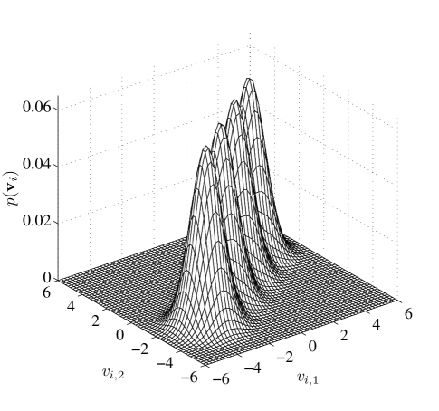
Figure 2: The multimodal Gaussian mixture PDF of ${\bf{v}}_{i}=[v_{i,1},v_{i,2}]^{T}$ for a $N_{t}=N_{r}=2$ MIMO system. For visualization purpose, the real-valued $4$PAM modulation with constellation $\mathcal{A}=\{{-3,-1,1,3}\}$ is used. $s_{1}$ is assumed to be detected, $s_{2}$ is the interference signal to $s_{1}$, and the real-valued Gaussian channel vectors ${\bf{h}}_{1}=[0.8884,-1.1471]^{T}$, ${\bf{h}}_{2}=[-1.0689,-0.8095]^{T}$. The possible interference patterns are $\underline{\bf{u}}_{1,1}=[3.2066,2.4285]^{T}$, $\underline{\bf{u}}_{1,2}=[1.0689,0.8095]^{T}$, $\underline{\bf{u}}_{1,3}=[-1.0689,-0.8095]^{T}$, $\underline{\bf{u}}_{1,4}=[-3.2066,-2.4285]^{T}$, and a given a priori probability vector ${\bf{P}}_{n}=[0.25,0.25,0.25,0.25]$ is used for the possible interference patterns. The means of the four component Gaussian distributions are $\underline{\bf{u}}_{1,1}$, $\underline{\bf{u}}_{1,2}$, $\underline{\bf{u}}_{1,3}$, $\underline{\bf{u}}_{1,4}$, respectively, and the covariance matrices of the four component Gaussian distributions are all $\sigma^{2}\bf{I}$ where $\sigma^{2}=0.631$.

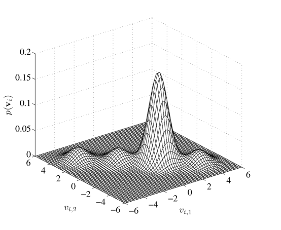
Figure 3: The multimodal Gaussian mixture PDF of ${\bf{v}}_{i}=[v_{i,1},v_{i,2}]^{T}$ for a $N_{t}=N_{r}=2$ MIMO system after iteration. For visualization purpose, the real-valued $4$PAM modulation with constellation $\mathcal{A}=\{{-3,-1,1,3}\}$ is used. $s_{1}$ is assumed to be detected, $s_{2}$ is the interference signal to $s_{1}$, and the real-valued Gaussian channel vectors ${\bf{h}}_{1}=[-3.0292,-0.4570]^{T}$, ${\bf{h}}_{2}=[1.2424,-1.0667]^{T}$. The possible interference patterns are $\underline{\bf{u}}_{1,1}=[-3.7273,3.2001]^{T}$, $\underline{\bf{u}}_{1,2}=[-1.2424,1.0667]^{T}$, $\underline{\bf{u}}_{1,3}=[1.2424,-1.0667]^{T}$, $\underline{\bf{u}}_{1,4}=[3.7273,-3.2001]^{T}$, and a given a priori probability vector ${\bf{P}}_{n}=[0.1,0.1,0.7,0.1]$ is used for the possible interference patterns. The means of the four component Gaussian distributions are $\underline{\bf{u}}_{1,1}$, $\underline{\bf{u}}_{1,2}$, $\underline{\bf{u}}_{1,3}$, $\underline{\bf{u}}_{1,4}$, respectively, and the covariance matrices of the four component Gaussian distributions are all $\sigma^{2}\bf{I}$ where $\sigma^{2}=0.631$.

IV The Proposed AB-Log-PDA Relying On A Priori Soft Feedback From the FEC Decoder

Based on the interference-plus-noise distribution analysis of Section III, below we will elaborate on the proposed low-complexity AB-Log-PDA algorithm. This algorithm uses the received signal $\bf{y}$, the channel matrix $\bf{H}$, as well as the a priori soft feedback gleaned from the FEC decoder, representing the soft estimates of the transmitted symbols ${\{s_{i}\}}_{i=1,\cdots,N_{t}}$, as its input parameters, and generates the estimated decision probabilities for ${\{s_{i}\}}_{i=1,\cdots,N_{t}}$ as its output.

As mentioned in Section III, if we can estimate the distribution of the interfering symbols $\{s_{k}\}_{k\neq i}$, the performance degradation imposed by ${\bf{u}}_{i}$ may be mitigated. Although initially we do not have any a priori knowledge about the distribution of $\{s_{k}\}_{k\neq i}$, we know exactly the distribution of the noise $\bf{n}$ and we are also aware of the legitimate values of $\{s_{k}\}_{k\neq i}$. Hence it is feasible to generate a coarse estimate of ${\{s_{i}\}}_{i=1,\cdots,N_{t}}$ relying solely on the knowledge of the noise distribution and the modulation constellation $\mathcal{A}$ at the beginning. Based on these observations, we may assume that the interference-plus-noise term ${\bf{v}}_{i}$ obeys a single $N_{r}$-variate Gaussian distribution. In order to fully characterize the complex random vector ${\bf{v}}_{i}$, which is not necessarily proper, we specify the mean as

$${\boldsymbol{\mu}}_{i}\triangleq\mathbb{E}({{\bf{v}}_{i}})=\sum\limits_{k\neq i}{\mathbb{E}(s_{k})}{\bf{h}}_{k},$$ (10)

the covariance as

$${\boldsymbol{\Upsilon}}_{i}\triangleq\mathbb{C}({\bf{v}}_{i})=\sum\limits_{k\neq i}\mathbb{C}(s_{k}){\bf{h}}_{k}{\bf{h}}_{k}^{H}+2\sigma^{2}{\bf{I}}_{N_{r}},$$ (11)

and the pseudo-covariance as

$${\underline{\boldsymbol{\Upsilon}}}_{i}\triangleq{\mathbb{C}_{p}}({\bf{v}}_{i})=\sum\limits_{k\neq i}\mathbb{C}_{p}(s_{k}){\bf{h}}_{k}{\bf{h}}_{k}^{T}.$$ (12)

We define an $(N_{t}\times M)$-element probability matrix ${\bf{P}}^{(z,z^{\prime})}$, whose $(i,m)$-th element $P_{m}^{(z,z^{\prime})}(s_{i}|{\bf{y}})\triangleq P^{(z,z^{\prime})}(s_{i}=a_{m}|{\bf{y}})$ is the estimate of the probability that we have $s_{i}=a_{m}$ at the $(z,z^{\prime})$-th iteration. More specifically, the integer $z^{\prime}\geq 0$ denotes the inner iteration index of the AB-Log-PDA, while the integer $z\geq 0$ is the index of the outer iteration between the AB-Log-PDA and the soft FEC decoder, $i=1,\cdots,N_{t}$ and $m=1,\cdots,M$. Then, the $\mathbb{E}(s_{k})$, ${\mathbb{C}}(s_{k})$ and $\mathbb{C}_{p}(s_{k})$ in (10), (11) and (12) are given by

$$\mathbb{E}(s_{k})=\sum\limits_{m=1}^{M}{a_{m}P^{(z,z^{\prime})}(s_{k}=a_{m}|{\bf{y}})},$$ (13)

$${\mathbb{C}}(s_{k})=\sum\limits_{m=1}^{M}{[a_{m}-\mathbb{E}(s_{k})][a_{m}-\mathbb{E}(s_{k})]^{*}P^{(z,z^{\prime})}(s_{k}=a_{m}|{\bf{y}})},$$ (14)

and

$$\mathbb{C}_{p}(s_{k})=\sum\limits_{m=1}^{M}{[a_{m}-\mathbb{E}(s_{k})]^{2}P^{(z,z^{\prime})}(s_{k}=a_{m}|{\bf{y}})},$$ (15)

respectively.

Note that Eq. (10) - Eq. (15) effectively use $(N_{t}-1)$ probability vectors $\{{\bf{P}}^{(z,z^{\prime})}(k,:)\}_{k\neq i}$ associated with the interfering signal $\{s_{k}\}_{k\neq i}$ to model ${\bf{v}}_{i}$. Since we do not have any outer a priori knowledge about the distribution of $s_{i}|\bf{y}$ at the beginning, an all-zero LLR vector will be provided as the input to the AB-Log-PDA, which is equivalent to initializing $P^{(z,z^{\prime})}(s_{i}=a_{m}|{\bf{y}})$ with a uniform distribution, i.e.

$$P^{(0,0)}(s_{i}=a_{m}|{\bf{y}})=\frac{1}{M},$$ (16)

$\forall i=1,\cdots,N_{t}$ and $\forall m=1,\cdots,M$.

Based on the assumption that ${\bf{v}}_{i}$ obeys the Gaussian distribution, ${\bf{y}}|s_{i}$ is also Gaussian distributed. Let us now define

$${\bf{w}}\triangleq{\bf{y}}-s_{i}{\bf{h}}_{i}-\sum\limits_{k\neq i}{\mathbb{E}(s_{k}){\bf{h}}_{k}}$$ (17)

and

$$\beta_{m,i}^{(z,z^{\prime}+1)}\triangleq{-\left[{\begin{array}[]{*{20}c}{\Re({\bf{w}})}\\ {\Im({\bf{w}})}\\ \end{array}}\right]^{T}{\bf{\Lambda}}_{i}^{-1}\left[{\begin{array}[]{*{20}c}{\Re({\bf{w}})}\\ {\Im({\bf{w}})}\\ \end{array}}\right]},$$ (18)

in which the composite covariance matrix ${\bf{\Lambda}}_{i}$ is defined as [15]

$${\bf{\Lambda}}_{i}\buildrel\Delta\over{=}\left[{\begin{array}[]{*{20}c}{\Re\left(\boldsymbol{\Upsilon}_{i}+\underline{\boldsymbol{\Upsilon}}_{i}\right)}&{-\Im\left(\boldsymbol{\Upsilon}_{i}-\underline{\boldsymbol{\Upsilon}}_{i}\right)}\\ {\Im\left(\boldsymbol{\Upsilon}_{i}+\underline{\boldsymbol{\Upsilon}}_{i}\right)}&{\Re\left(\boldsymbol{\Upsilon}_{i}-\underline{\boldsymbol{\Upsilon}}_{i}\right)}\\ \end{array}}\right],$$ (19)

where $\Re(\cdot)$ and $\Im(\cdot)$ represent the real and imaginary part of a complex variable, respectively. Then the likelihood function of ${\bf{y}}|s_{i}=a_{m}$ at the $(z,z^{\prime}+1)$-st iteration satisfies

$$p^{(z,z^{\prime}+1)}({\bf{y}}|s_{i}=a_{m})\propto\exp\left(\beta_{m,i}^{(z,z^{\prime}+1)}\right),$$ (20)

where the symbol “$\propto$” means “proportional to”.

Upon invoking an approximate form of the Bayesian theorem[12, 13], the estimated probability of symbol $s_{i}$ at the $(z,z^{\prime}+1)$-st iteration may be calculated as

$$P^{(z,z^{\prime}+1)}(s_{i}=a_{m}|{\bf{y}})$$ (21)

$$\approx \frac{{p^{(z,z^{\prime}+1)}({\bf{y}}|s_{i}=a_{m})}}{{\sum\limits_{m=1}^{M}{p^{(z,z^{\prime}+1)}({\bf{y}}|s_{i}=a_{m})}}}$$

$$= \frac{\exp\left(\beta_{m,i}^{(z,z^{\prime}+1)}-\gamma\right)}{{\sum\limits_{m=1}^{M}{\exp\left(\beta_{m,i}^{(z,z^{\prime}+1)}-\gamma\right)}}},$$

where $\gamma\triangleq\max\limits_{m=1,\cdots,M}{\beta_{m,i}^{(z,z^{\prime}+1)}}$ is subtracted from $\beta_{m,i}^{(z,z^{\prime}+1)}$ for enhancing the numerical stability.

TABLE I: Summary of the AB-Log-PDA based IDD algorithm

Given the received signal $\bf{y}$, the channel matrix $\bf{H}$ and the constellation $\mathcal{A}$.

Step 1. Set the initial values of the inner iteration index and outer iteration

index to $z^{\prime}=0$ and $z=0$, respectively. Initialize the bit-based a priori LLRs

feedback from the FEC decoder as zeros.

Step 2. Convert the a priori LLRs feedback from the FEC decoder to symbol

probabilities shown in probability matrix ${\bf{P}}^{(z,z^{\prime})}$.

Step 3. Using the values of $\left\{{{\bf{P}}^{(z,z^{\prime})}(k,:)}\right\}_{k\neq i}$, calculate $P_{m}^{(z,z^{\prime}+1)}(s_{i}|{\bf{y}})$ by

for $i=1:N_{t}$

calculate the statistics of the interference-plus-noise term ${\bf{v}}_{i}$ using

(10) - (15), as well as the inverse of ${\bf{\Lambda}}_{i}$ in (19),

for $m=1:M$

calculate $P_{m}^{(z,z^{\prime}+1)}(s_{i}|{\bf{y}})$ using (17), (18), (22) and (24).

end

end

Step 4. If $z^{\prime}$ has reached a given number of inner iterations, go to Step 5.

Otherwise, let $z^{\prime}\leftarrow z^{\prime}+1$, and return to Step 3.

Step 5. Convert the symbol probabilities $P_{m}^{(z,z^{\prime}+1)}(s_{i}|{\bf{y}})$ to bit-based

LLRs, of which the extrinsic parts are delivered to the outer FEC decoder.

If $z$ has reach a given number of outer iterations, make hard decisions using the

soft output of the FEC decoder. Otherwise, let $z\leftarrow z+1$, and return to Step 2.

As a further effort to improve the achievable numerical stability and accuracy, the logarithmic-domain form of (21) is formulated as

$$\psi_{m,i}^{(z,z^{\prime}+1)} \triangleq \ln\left[P^{(z,z^{\prime}+1)}(s_{i}=a_{m}|{\bf{y}})\right]$$ (22)

$$= {\tilde{\beta}}_{m,i}^{(z,z^{\prime}+1)}-\ln\left[\sum\limits_{m=1}^{M}{\exp\left({\tilde{\beta}}_{m,i}^{(z,z^{\prime}+1)}\right)}\right],$$

in which we have ${\tilde{\beta}}_{m,i}^{(z,z^{\prime}+1)}\triangleq\beta_{m,i}^{(z,z^{\prime}+1)}-\gamma$, and the second term of the right-hand-side expression may be computed by invoking the “Jacobian logarithm” of [8]. Alternatively, upon employing the Max-log approximation, (22) may be further simplified to

$$\psi_{m,i}^{(z,z^{\prime}+1)}\approx{\tilde{\beta}}_{m,i}^{(z,z^{\prime}+1)}.$$ (23)

As a result, the estimated decision probability of $s_{i}$ relying on (22) and (23) is given by

$$P^{(z,z^{\prime}+1)}(s_{i}=a_{m}|{\bf{y}})\approx e^{\psi_{m,i}^{(z,z^{\prime}+1)}},$$ (24)

which will update the value of $P^{(z,z^{\prime})}(s_{i}=a_{m}|{\bf{y}})$ in the probability matrix ${\bf{P}}^{(z,z^{\prime})}$. Following the inner iterations within the AB-Log-PDA, if any, the updated symbol probabilities have to be converted to the equivalent bit-based LLRs, whose extrinsic constituent will be delivered to the outer FEC decoder of Fig. 1. In turn, the extrinsic LLRs output by the FEC decoder will be converted to symbol probabilities in the next outer iteration, before feeding them into the AB-Log-PDA for generating new estimates of the symbol probabilities. For reasons of explicit clarity, the AB-Log-PDA algorithm relying on the a priori soft feedback generated by the FEC decoder of Fig. 1 is summarized in Table I.

V Extrinsic LLR Calculation for AB-Log-PDA in FEC-Coded MIMO Systems

In order to integrate the AB-Log-PDA into the IDD scheme, the AB-Log-PDA has to output correct extrinsic LLRs for each of the FEC-coded bits, which is however, not quite as straightforward as it seems at first sight, given that the output probabilities of the PDA were interpreted as APPs in [12, 13, 14, 15, 16, 17]. We assume that the components of the transmitted symbol-vector $\bf{s}$ are obtained using the bit-to-symbol mapping function of $s_{i}=\textrm{map}\left({{\bf{b}}_{i}}\right)$, $i=1,2,\cdots,N_{t}$, where ${\bf{b}}_{i}=\left[{b_{i,1},b_{i,2},\cdots,b_{il},\cdots,b_{i,M_{b}}}\right]^{T}$ $\in\left\{{+1,-1}\right\}^{M_{b}}$ is the vector of bits mapped to symbol $s_{i}$. Additionally, we denote the vector of bits corresponding to $\bf{s}$ as $\bf{b}$, which satisfies $\bf{s}=\textrm{map}\left({\bf{b}}\right)$ and is formed by concatenating the $N_{t}$ antennas’ bit vectors ${\bf{b}}_{1},{\bf{b}}_{2},\cdots,{\bf{b}}_{N_{t}}$, yielding ${\bf{b}}=\left[{{\bf{b}}_{1}^{T},{\bf{b}}_{2}^{T},\cdots,{\bf{b}}_{N_{t}}^{T}}\right]^{T}=\left[{b_{1},b_{2},\cdots,b_{k},\cdots,b_{M_{b}N_{t}}}\right]^{T}\in\left\{{+1,-1}\right\}^{M_{b}N_{t}}$. Hence the indices of $b_{il}$ and $b_{k}$ are related to each other by $k={M_{b}}(i-1)+l$.

Note that the AB-Log-PDA algorithm finally outputs the estimated symbol probabilities of $P(s_{i}=a_{m}|{\bf{y}})$, where the iteration indices are omitted without causing any confusion. Additionally, it provides the likelihood functions of $p({\bf{y}}|s_{i}=a_{m})$ conditioned on $s_{i}$ as its intermediate output. By contrast, the classic candidate-search based approach outputs the likelihood function of $p({\bf{y}}|{\bf{b}})$ [or equivalently, $p({\bf{y}}|{\bf{s}})$] conditioned on the bit vector $\bf{b}$ (or symbol vector $\bf{s}$), and calculates the bit-based extrinsic LLRs by using $p({\bf{y}}|{\bf{b}})$ [or $p({\bf{y}}|{\bf{s}})$]. Below we will demonstrate that the candidate-search based approach of computing the bit-based extrinsic LLRs is not feasible for the AB-Log-PDA algorithm. In other words, we cannot obtain $p({\bf{y}}|{\bf{b}})$ or $p({\bf{y}}|{\bf{s}})$ based on $P(s_{i}=a_{m}|{\bf{y}})$ and/or $p({\bf{y}}|s_{i}=a_{m})$. Instead, we will demonstrate that there exists a simpler method of directly obtaining the bit-based extrinsic LLRs based on the output of the AB-Log-PDA.

V-A Challenges in Calculating Extrinsic LLRs for the PDA Based Methods

In principle, for a MIMO system characterized by Eq. (1), the classic approach of deriving bit-based extrinsic LLRs is based on the likelihood function of $p({\bf{y}}|{\bf{b}})$ or $p({\bf{y}}|{\bf{s}})$. Specifically, the extrinsic LLR of $b_{il}$ (or $b_{k}$) is given by [8]

$$L_{E}(b_{il}|{\bf{y}})=L_{E}(b_{k}|{\bf{y}})=\ln\frac{\sum\limits_{\forall{\bf{b}}\in\mathbb{B}_{k}^{+}}p({\bf{y}}|{\bf{b}})\exp(\frac{1}{2}{\bf{b}}_{[k]}^{T}{\bf{L}}_{A,[k]})}{\sum\limits_{\forall{\bf{b}}\in\mathbb{B}_{k}^{-}}p({\bf{y}}|{\bf{b}})\exp(\frac{1}{2}{\bf{b}}_{[k]}^{T}{\bf{L}}_{A,[k]})},$$ (25)

where $\mathbb{B}_{k}^{\pm}$ denotes the set of $2^{N_{t}M_{b}-1}$ legitimate bit vectors $\bf{b}$ having $b_{k}=\pm 1$, and ${\bf{b}}_{[k]}=[b_{1},\cdots,$ $b_{j},\cdots,b_{N_{t}M_{b}}]_{j\neq k}^{T}$ represents a truncated version of $\bf{b}$ excluding $b_{k}$, while ${\bf{L}}_{A,[k]}$ represents the a priori LLRs corresponding to ${\bf{b}}_{[k]}$. Eq. (25) indicates that $L_{E}(b_{k}|{\bf{y}})$ is determined by $p({\bf{y}}|{\bf{b}})$, and by the a priori LLRs of the other bits conveyed by a single symbol vector $\bf{s}$. However, below we will prove that it is infeasible to invoke this approach to calculate bit-based extrinsic LLRs for the family of PDA based algorithms including the AB-Log-PDA.

Proposition 1.

For all PDA algorithms which output the probabilities $P(s_{i}|{\bf{y}})$, or the likelihood functions $p({\bf{y}}|s_{i})$, the bit-based extrinsic LLR $L_{E}(b_{k}|{\bf{y}})$ cannot be calculated using the candidate-search method which relies on $p({\bf{y}}|\bf{b})$ or $p({\bf{y}}|\bf{s})$.

Proof:

Define a non-zero random vector ${\bf{s}}=[s_{1},s_{2},\cdots,s_{N_{t}}]^{T}$, and a non-zero random vector $\bf{y}$, where $s_{i}$ and $s_{j}$ are independent of each other in the absence of a priori knowledge, $i\neq j$, $i,j=1,\cdots,N_{t}$, and assume that $\bf{y}$ is associated with $\bf{s}$ by the function of ${\bf{y}}=f({\bf{s}})$. We have

$$P({\bf{y}}|{\bf{s}}) = P({\bf{y}}|s_{1},s_{2},\cdots,s_{N_{t}})$$ (26)

$$= \frac{P({\bf{y}},s_{1},s_{2},\cdots,s_{N_{t}})}{P(s_{1},s_{2},\cdots,s_{N_{t}})}$$

$$= \frac{P(s_{1}|{\bf{y}})P(s_{2},\cdots,s_{N_{t}}|{\bf{y}},s_{1})P({\bf{y}})}{P(s_{1})P(s_{2})\cdots P(s_{N_{t}})},$$

where $P(s_{2},\cdots,s_{N_{t}}|{\bf{y}},s_{1})$ can be further expanded as

$$P(s_{2}|{\bf{y}},s_{1})P(s_{3}|{\bf{y}},s_{1},s_{2})\cdots P(s_{N_{t}}|{\bf{y}},s_{1},s_{2},\cdots,s_{N_{t}-1}).$$ (27)

Note that the conditions $s_{i}$ associated with each single probability in (27) cannot be removed, which implies that it is infeasible to further simplify each probability in (27). In other words, we have $P({\bf{s}}|{\bf{y}})\neq P(s_{1}|{\bf{y}})P(s_{2}|{\bf{y}})\cdots P(s_{N_{t}}|{\bf{y}})$, which implies that in a converging connection of the acyclic, directed graph representation of Bayesian Networks, the presence of knowledge as regards to the child-node makes the parent-nodes conditionally dependent. Again, this is a standard result in Bayesian Networks [24]. Therefore, the probability $P({\bf{y}}|{\bf{s}})$ cannot be exactly expressed as a function of any probabilities of $P(s_{i})$, $P(\bf{y})$, $P({\bf{y}}|s_{i})$ and/or $P(s_{i}|{\bf{y}})$. Hence the proof of Proposition 1 is established. ∎

V-B Calculating Extrinsic LLRs for AB-Log-PDA

Due to Proposition 1, the candidate-search based approach of calculating bit-based extrinsic LLRs is not applicable to the family of PDA algorithms. Let $\mathcal{A}_{l}^{\pm}$ denote the set of $M/2$ constellation points whose $l$-th bit is $\pm 1$. Then, alternatively, the extrinsic LLR of $b_{il}$ may be rewritten as

$$L_{E}(b_{il}|{\bf{y}})=\underbrace{\ln\frac{\sum\limits_{\forall a_{m}\in\mathcal{A}_{l}^{+}}P(s_{i}=a_{m}|{\bf{y}})}{\sum\limits_{\forall a_{m}\in\mathcal{A}_{l}^{-}}P(s_{i}=a_{m}|{\bf{y}})}}_{L_{D}(b_{il}|{\bf{y}})}-\underbrace{\ln\frac{P(b_{il}=+1)}{P(b_{il}=-1)}}_{L_{A}(b_{il})},$$ (28)

where $L_{D}(b_{il}|{\bf{y}})$ and $L_{A}(b_{il})$ denote the a posteriori and a priori LLRs of $b_{il}$, respectively. It is noteworthy that (28) represents a simple approach of generating the bit-based extrinsic LLR of $L_{E}(b_{il}|{\bf{y}})$, as long as the true symbol APP of $P(s_{i}=a_{m}|{\bf{y}})$ can be obtained.

However, although we can directly obtain the estimated symbol probabilities of $P(s_{i}=a_{m}|{\bf{y}})$ from the output of the AB-Log-PDA, as shown in (21), our study shows that this sort of estimated symbol probabilities, interpreted as symbol APPs in [12, 13, 14, 15, 16, 17], fail to generate the correct bit-based extrinsic LLRs, when invoking (28). Therefore, the results of (21) should not be interpreted as symbol APPs satisfying (28), but rather as the normalized symbol likelihoods. Based on this insight, the bit-based extrinsic LLRs of the AB-Log-PDA may be obtained by directly employing the approximate Bayesian Theorem based symbol probabilities of (21) as follows.

Conjecture 1.

The bit-based extrinsic LLR of the AB-Log-PDA algorithm relying on (21) is given by

$$L_{E}(b_{il}|{\bf{y}})\approx\ln\frac{\sum\limits_{\forall a_{m}\in\mathcal{A}_{l}^{+}}P(s_{i}=a_{m}|{\bf{y}})}{\sum\limits_{\forall a_{m}\in\mathcal{A}_{l}^{-}}P(s_{i}=a_{m}|{\bf{y}})},$$ (29)

where $P(s_{i}=a_{m}|{\bf{y}})$ is calculated by invoking (24).

The $L_{E}(b_{il}|{\bf{y}})$ values calculated from (29) using the normalized symbol likelihoods are typically not equivalent to $L_{E}(b_{il}|{\bf{y}})$ calculated from (28) using the true symbol APPs, but nonetheless, they constitute a good approximation of the latter without inducing any significant performance loss, as it will be demonstrated by our simulations in Section VI. As a result, the classic IDD receiver structure is simplified, as shown in Fig. 1, where we have ${\bf{L}}_{E_{2}}={\bf{L}}_{D_{2}}$, rather than ${\bf{L}}_{E_{2}}={\bf{L}}_{D_{2}}-{\bf{L}}_{A_{2}}$.

VI Simulation Results and Discussions

In this section, the performance of the proposed AB-Log-PDA based IDD scheme is characterized with the aid of both semi-analytical extrinsic information transfer (EXIT) charts and Monte-Carlo simulations. Additionally, the complexity of the proposed AB-Log-PDA based IDD scheme is analyzed, which further confirms the attractive performance versus complexity tradeoff achieved by the proposed AB-Log-PDA based IDD scheme. The FEC employed is the parallel concatenated recursive systematic convolutional (RSC) code based turbo code having a coding rate of $R=\frac{k}{n}=1/2$, constraint length of $L=3$ and generator polynomials of $(7,5)$ in octal form. The turbo code is decoded by the Approximate-Log-MAP algorithm using $it_{tc}=4$ inner iterations. The interleaver employed is the $2400$-bit random sequence interleaver. The remaining scenario-dependent simulation parameters are shown in the respective figures, where the MIMO arrangement is represented in form of $(N_{t}\times N_{r})$.

VI-A Performance of the AB-Log-PDA based IDD

1) Impact of inner PDA iterations

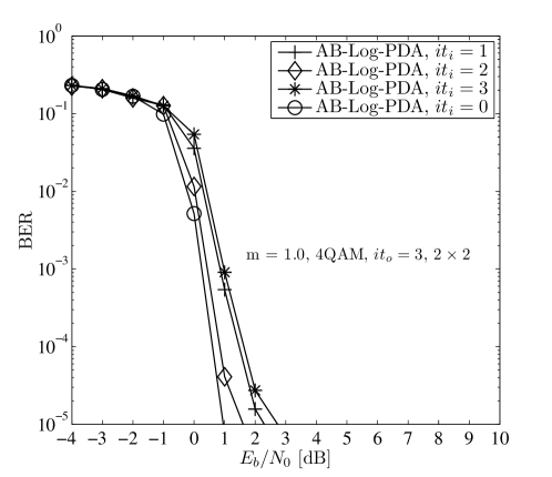
Figure 4: Impact of the number of inner iterations on the achievable BER of the AB-Log-PDA based IDD schemes.

In Fig. 4, we investigate the impact of the number of inner iterations within the AB-Log-PDA algorithm on the achievable performance of the IDD scheme, which is degraded upon increasing the number of inner iterations of the AB-Log-PDA, despite the fact that the computational complexity increases dramatically. This implies that the optimal number of inner iterations of the AB-Log-PDA conceived for the IDD receiver is $it_{i}=z^{\prime}=0$. It should be noted that for other types of iterative receivers, the inner iterations often refer to the iterations within the FEC-decoder, in which typically the MAP algorithm and its variants are employed. In that context, increasing the number of inner iterations typically improves the iterative receiver’s performance, which is in contrast to the impact of the inner PDA detector’s iterations, as shown in Fig. 4.

The reasons as to why the inner PDA iterations fail to provide BER improvement can be understood from three different perspectives, as detailed below.

i) The PDA method is reconfigurable, and both the inner PDA iterations as well as the outer iterations play a similar role with respect to the PDA detector module in our IDD scenario, but the soft information provided by the two sorts of iterations has a different quality. Firstly, when the number of IAI components is insufficiently high for the central limit theorem to prevail, there is an inevitable Gaussian approximation error, even if the PDA method has converged to its best possible estimate. This approximation error is more severe, when the soft information provided by the Gaussian approximation in each inner PDA iteration is unreliable, because error propagation will occur during the process of inner PDA iterations. Furthermore, if we look at the PDA detector module in isolation, the inner PDA iterations and the outer iterations play a similar role – both of them are responsible for providing the input soft information for the next round of Gaussian approximation. This Gaussian approximation procedure is identical for the two sorts of iterations, while the quality of the soft information provided by the two types of iterations is different. Additionally, compared to the scenario of uncoded systems, where the PDA method can only rely on its own knowledge of the transmitted/received signal and its own inner iterations, in FEC-coded systems the Gaussian approximation error can be mitigated more effectively by the improved-reliability soft information fed back by the FEC decoder. Therefore, the inner PDA iterations can be replaced by the more efficient outer iterations in the IDD scenario considered.

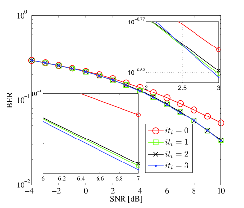
Figure 5: Observation of the fine details of the impact of inner PDA iterations on the achievable performance of a PDA-based detector in an uncoded MIMO system, where we have $N_{t}=N_{r}=2$, and $4$QAM is used.

ii) The convergence profile of the PDA method is not monotonic. In engineering/optimization problems two typical types of convergence behaviors may be observed for a function/sequence. Namely, the function/sequence may monotonically approach its optimum, or may fluctuate during the process of approaching its optimum — hopefully without getting trapped in a local optimum. Upon observing Fig. 5 as to the fine details of the impact of inner PDA iterations on the achievable performance of the PDA detector in an uncoded MIMO system, we find that the convergence behavior of the PDA method belongs to the second type. This particular convergence behavior of the PDA has not been reported in the open literature, because in uncoded systems hard decisions are made based on the output symbol probabilities of the PDA method. Hence the resultant BER performance fluctuation may remain so trivial that it may be regarded as being unchanged after several inner PDA iterations. However, as we can see from Fig. 5, the BER performance of $it_{i}=1,2,3$ actually exhibits some degree of fluctuations.

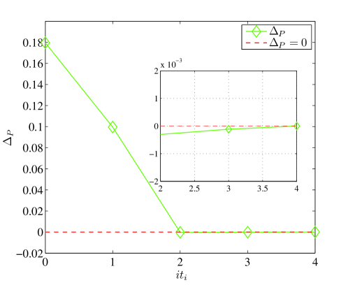
Figure 6: Observation of the fine details of the probability convergence profile: the probability gap between the previous iteration and the current iteration of a PDA-based detector when we look at a single symbol probability $P(s_{i}=a_{m}|{\bf{y}})$ in an uncoded MIMO systems, where we have $N_{t}=N_{r}=2$, $4$QAM.

These fluctuations can be further confirmed by tracking the changes of a single symbol’s probability $P(s_{i}=a_{m}|{\bf{y}})$ during the inner PDA iterations, as shown in Fig. 6. In uncoded systems, the PDA method is regarded to be converged when the probability changes obey $\Delta P=|P(\textrm{current iteration})-P(\textrm{previous iteration})|<\epsilon$, where the threshold $\epsilon$ is a small positive real number. In Fig. 6 we show how $\Delta P$ changes upon increasing the number of inner PDA iterations in the context of a $4$QAM aided uncoded $(2\times 2)$-element MIMO system, where we have $\epsilon=0.001$. Again, although a superficial observation shows that $\Delta P$ remains more or less unchanged after two iterations, $\Delta P$ actually exhibits a modest fluctuation, because we have both positive and negative values of $\Delta P$ during the iterations.

However, the trivial fluctuation at the soft output of the PDA detector module may induce an augmented BER fluctuation at the output of the FEC-coded system. Let us consider for example a symbol probability vector of ${\bf{p}}_{1}=[0.35,0.58,0.06,0.01]$, which represents our belief as regards to $s_{i}=a_{1},a_{2},a_{3},a_{4}$, respectively. In uncoded systems, what we care about is, which specific probability is the maximum. In this case we will choose $s_{i}=a_{2}$, and a modest fluctuation from ${\bf{p}}_{1}$ to ${\bf{p}}_{2}=[0.38,0.53,0.06,0.01]$ will not lead to a different decision. However, in FEC-coded systems, we care about both the amplitude and the sign of the LLRs. A modest fluctuation in the probability vector ${\bf{p}}_{1}$ may alter some of the resultant LLRs that are near zero, so that they fluctuate between positive/negative values and hence might cause more severe decision errors.

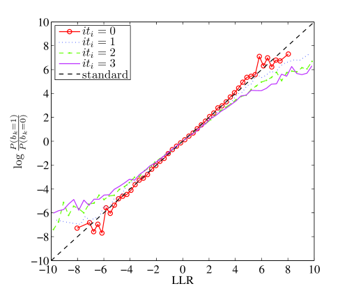
Figure 7: The impact of inner PDA iterations on the consistency of LLRs output by the AB-Log-PDA detector.

iii) The inner PDA iterations degrade the quality of the LLRs output by the AB-Log-PDA. In Fig. 7 we show the impact of the inner PDA iterations on the quality of the LLRs at the output of the AB-Log-PDA by testing the so-called consistency condition [25] of these LLRs. As seen from Fig. 7, the consistency profile of the LLRs at the output of the AB-Log-PDA is degraded upon increasing the number of inner PDA iterations. This observation provides another perspective, confirming that it may in fact be detrimental to include inner PDA iterations, when a PDA-based IDD receiver is considered in FEC-coded systems. Therefore, we dispense with inner iterations in the AB-Log-PDA and set $it_{i}=0$ in our forthcoming simulations.

2) Impact of outer iterations

Fig. 8 compares the convergence behavior of the proposed AB-Log-PDA based IDD with $it_{i}=0$ and that of the optimal Exact-Log-MAP based IDD scheme using EXIT chart [26] analysis, where the EXIT curve of the AB-Log-PDA is close to that of the Exact-Log-MAP. For example, when the a priori mutual information is $I_{A,inner}=0$, the extrinsic mutual information of the AB-Log-PDA and of the Exact-Log-MAP is $I_{E,outer}=0.5332$ and $I_{E,outer}=0.5596$, respectively. This indicates that the performance of the AB-Log-PDA is close to that of the Exact-Log-MAP in the scenario considered. Additionally, the detection/decoding trajectories indicate that both the AB-Log-PDA and the Exact-Log-MAP based IDD schemes converge after three iterations, although the respective performance improvements achieved at each iteration are different.

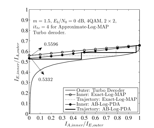
Figure 8: EXIT chart analysis of the AB-Log-PDA ($it_{i}=0$) and the Exact-Log-MAP based IDD schemes.

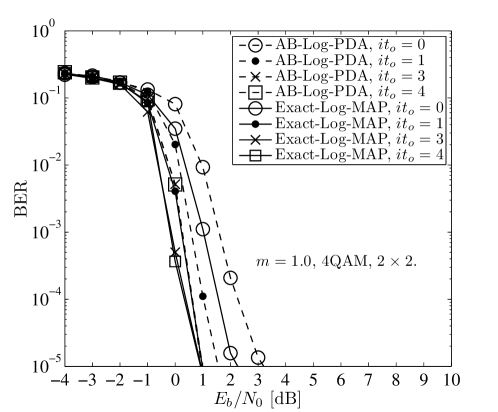
Figure 9: Impact of the number of outer iterations on the achievable BER of the AB-Log-PDA ($it_{i}=0$) and the Exact-Log-MAP based IDD schemes.

The above EXIT chart based performance prediction and the convergence behavior of the IDD schemes considered are also characterized by the BER performance results of Fig. 9, where the Nakagami-$m$ fading parameter is set to $m=1.0$, which corresponds to the Rayleigh fading channel. Observe from Fig. 9 that the performance of the AB-Log-PDA based IDD scheme is improved upon increasing the number of outer iterations $it_{o}$, where $it_{o}=0$ represents the conventional receiver structure in which the signal detector and the FEC decoder are serially concatenated, but operate without exchanging soft information. However, the attainable improvement gradually becomes smaller and the performance achieved after three outer iterations becomes almost the same as that of four outer iterations. This implies that the AB-Log-PDA based IDD scheme essentially converges after three outer iterations. A similar convergence profile is also observed for the optimal Exact-Log-MAP based IDD, although its performance is always marginally better than that of the corresponding AB-Log-PDA based IDD scheme. Notably, both IDD schemes considered achieve $\textrm{BER}=10^{-5}$ at about $E_{b}/N_{0}=1$ dB after three iterations.

3) Impact of Nakagami-$m$ fading parameter $m$

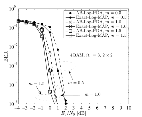
Figure 10: Impact of Nakagami-$m$ fading parameter $m$ on the achievable BER of the AB-Log-PDA ($it_{i}=0$) and the Exact-Log-MAP based IDD schemes.

Fig. 10 shows the impact of different $m$ values on the achievable BER performance of the IDD schemes considered. As $m$ decreases, the achievable performance of both the IDD schemes considered is degraded, since the fading becomes more severe. However, the performance gap between the AB-Log-PDA and the Exact-Log-MAP based IDD schemes is marginal for all values of $m$ considered.

4) Impact of modulation order

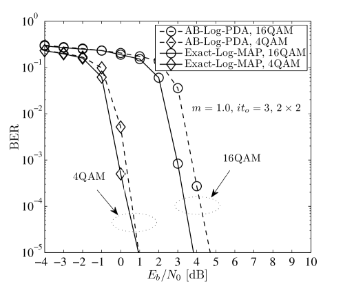
Figure 11: Impact of the modulation order on the achievable BER of the AB-Log-PDA ($it_{i}=0$) and the Exact-Log-MAP based IDD schemes.

Additionally, in Fig. 11 we investigate the impact of the modulation order on the achievable performance of the AB-Log-PDA based IDD scheme. It is observed that for higher-order modulation, for example, 16QAM, the performance gap between the AB-Log-PDA and the Exact-Log-MAP based IDDs becomes larger. This is because the accuracy of the Gaussian approximation in the PDA method degrades, when the modulation order is increased. More specifically, as analyzed in Section III and shown in Fig. 2 as well as Fig. 3, the interference-plus-noise term ${\bf{v}}_{i}$ obeys a multimodal Gaussian distribution associated with $M^{N_{t}-1}$ Gaussian component-distributions. When $M$ is large, there exist many interfering Gaussian component-distributions, where the effect of each might be trivial, but their accumulated effect may render the estimated $P(s_{i}=a_{m}|\bf{y})$ inaccurate, and hence inaccurate bit-based extrinsic LLRs might be calculated using (29).

5) Impact of the number of transmit antennas

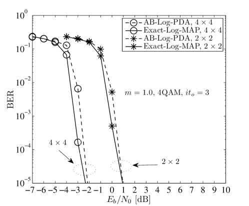
Figure 12: Impact of the number of transmit antennas on the achievable BER of the AB-Log-PDA ($it_{i}=0$) and the Exact-Log-MAP based IDD schemes.

The impact of the number of transmit antennas $N_{t}$ on the achievable performance of the AB-Log-PDA based IDD scheme is shown in Fig. 12. On the one hand, upon increasing $N_{t}$ (and $N_{r}$), an increased diversity gain is obtained, and a more accurate Gaussian approximation is achieved according to the central limit theorem. Hence we observe a significant performance improvement, when moving from a $(2\times 2)$-element to a $(4\times 4)$-element MIMO system. On the other hand, however, it is observed that when $N_{t}$ (and $N_{r}$) is increased, the performance gap between the AB-Log-PDA and the Exact-Log-MAP based IDD receivers is also increased. This is because the achievable diversity gain of the Exact-Log-MAP detector is higher than that of the AB-Log-PDA detector, although a higher $N_{t}$ results in an improved Gaussian approximation quality.

6) Impact of channel-estimation error

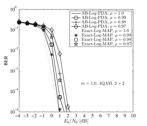
Figure 13: Impact of channel-estimation error on the achievable BER of the AB-Log-PDA ($it_{i}=0$) and the Exact-Log-MAP based IDD schemes.

Finally, the impact of the channel-estimation errors on the achievable BER performance of both the AB-Log-PDA and the Exact-Log-MAP based IDD schemes is investigated in Fig. 13. The estimated channel matrix is given by $\hat{\bf{H}}=\rho{\bf{H}}+\sqrt{(1.0-\rho^{2})}\Delta{\bf{H}}$, where $0\leq\rho\leq 1$ indicates the accuracy of channel-estimation. For example, $\rho=1.0$ represents perfect channel-estimation and each entry of $\Delta{\bf{H}}$ obeys a zero-mean, unit-variance complex Gaussian distribution. It can be observed from Fig. 13 that the achievable BER performance of both IDD schemes is moderately degraded upon increasing the value of $\rho$ and that the AB-Log-PDA based IDD still achieves a performance similar to that of its Exact-Log-MAP based IDD counterpart, even when the channel-estimation accuracy is as low as $\rho=0.97$.

VI-B Complexity Analysis

Because the turbo codec module is common to both IDD schemes, and since we have shown that both the AB-Log-PDA and the Exact-Log-MAP based IDD schemes converge after three iterations in the scenarios considered, the computational complexity of the proposed AB-Log-PDA based IDD scheme can be evaluated by simply comparing its complexity to that of the Exact-Log-MAP in a single iteration. As shown in Table I, the major computational cost of the AB-Log-PDA per transmit symbol is the calculation of ${\bf{\Lambda}}_{i}^{-1}$ and the matrix multiplication of (18). Direct calculation of ${\bf{\Lambda}}_{i}^{-1}$ imposes a computational cost of $\mathcal{O}(8N_{r}^{3})$ real-valued operations (additions/multiplications), which is still relatively expensive. Fortunately, by using the Sherman-Morrison-Woodbury formula based “speed-up” techniques of [12], the computational cost of calculating ${\bf{\Lambda}}_{i}^{-1}$ can be reduced to $\mathcal{O}(4N_{t}N_{r}^{2})$ real-valued operations per iteration. Additionally, the calculation of (18) requires $\mathcal{O}(4MN_{t}N_{r}^{2}+2MN_{t}N_{r})$ real-valued operations per iteration. In summary, the computational complexity of the AB-Log-PDA method is $\mathcal{O}(4MN_{t}N_{r}^{2}+2MN_{t}N_{r})$ + $\mathcal{O}(4N_{t}N_{r}^{2})$ per iteration.

By comparison, the Exact-Log-MAP algorithm has to calculate the Euclidean distance ${\|{\bf{y}}-{\bf{Hs}}\|}^{2}$ for $M^{N_{t}}$ times, hence its complexity order is $\mathcal{O}(M^{N_{t}})$. More specifically, ${\|{\bf{y}}-{\bf{Hs}}\|}^{2}$ requires $\mathcal{O}(4N_{r}N_{t}+6N_{r})$ real-valued operations. Therefore, the Exact-Log-MAP algorithm has a computational complexity of $\mathcal{O}[M^{N_{t}}(4N_{r}N_{t}+6N_{r})]$ real-valued operations per iteration, which is significantly higher than that of the AB-Log-PDA, especially when $N_{t}$, $N_{r}$ and $M$ have large values. This observation is further confirmed by the results of Fig. 14, where the computational complexity of the two algorithms is compared in terms of the number of real-valued operations $N_{RO}$, while considering the scenario of $N_{r}=N_{t}$ as an example. To elaborate a little further, the upper surface and the lower surface represent the computational complexity of the Exact-Log-MAP algorithm and of the proposed AB-Log-PDA algorithm, respectively. Since we assume $N_{r}=N_{t}$, the computational complexity of both algorithms becomes a function of the number of transmit antennas $N_{t}$ and of the modulation order $M$. We can observe from Fig. 14 that upon increasing $N_{t}$ and/or $M$, the computational complexity of the Exact-Log-MAP algorithm increases substantially faster than that of the AB-Log-PDA algorithm. Additionally, compared to $M$, $N_{t}$ plays a more significant role in determining the computational complexity of the two algorithms.

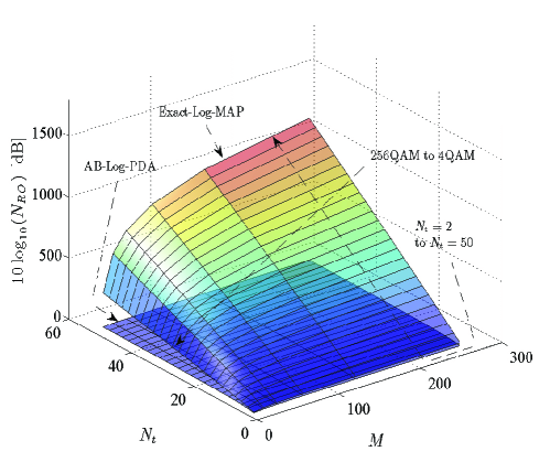
Figure 14: Computational complexity comparison of the AB-Log-PDA ($it_{i}=0$) and the Exact-Log-MAP algorithms in terms of the number of real operations $N_{RO}$.

Finally, compared to the popular list sphere decoding (LSD) algorithm [8], which has an exponential complexity lower bound, especially for low SNR values [27], the proposed AB-Log-PDA has the distinct advantage of a polynomial-time complexity (roughly a cubic function of $N_{t}$, as shown above) for all SNR values. Although there exist other reduced-complexity variants of LSD, such as the list fixed-complexity sphere-decoder (LFSD) [28] and the soft $K$-best sphere-decoder using an improved “look-ahead path metric” [29], in general they still have a higher complexity than the AB-Log-PDA algorithm if the SNR value is low and/or the problem size (i.e. $N_{t}$ and $M$) is large. This is because finding the closest point in lattices is an NP-hard problem [30]. To be more specific, the computational complexity of the $K$-best SD of [29] is indeed reduced, but it remains of similar order to that of the LFSD. which is on the order of $\mathcal{O}(M^{\sqrt{N}_{t}})$ [31].

VII Conclusions

We demonstrate that the classic candidate-search based method of calculating bit-based extrinsic LLRs is not applicable to the family of PDA-based detectors. Additionally, in stark contrast to the existing literature, we demonstrate that the output symbol probabilities of the existing PDAs are not the true APPs, they are rather constituted by the normalized symbol likelihoods. Hence, surprisingly, the classic relationship, where the extrinsic LLRs are given by subtracting the a priori LLRs from the a posteriori LLRs does not hold for the existing PDA-based detectors, when the output probabilities of the existing PDAs are interpreted as APPs to generate a posteriori LLRs. Based on these insights, we conceive the AB-Log-PDA method and identify the technique of calculating the bit-based extrinsic LLRs for the AB-Log-PDA, which results in a simplified IDD receiver structure. Additionally, we demonstrate that we may completely dispense with any inner iterations within the AB-Log-PDA in the context of IDD receivers. Our complexity analysis and numerical results recorded for transmission over Nakagami-$m$ fading MIMO channels demonstrate that the proposed AB-Log-PDA based IDD scheme is capable of achieving a comparable performance to that of the optimal MAP detector based IDD receiver, while imposing a significantly lower computational complexity in the scenarios considered.

Shaoshi Yang (S’09) received the B.Eng. Degree in information engineering from Beijing University of Posts and Telecommunications, Beijing, China, in 2006. He is currently working toward the Ph.D. degree in wireless communications with the School of Electronics and Computer Science, University of Southampton, Southampton, U.K., through scholarships from both the University of Southampton and the China Scholarship Council. From November 2008 to February 2009, he was an Intern Research Fellow with the Communications Technology Laboratory, Intel Labs China, Beijing, where he focused on Channel Quality Indicator Channel design for mobile WiMAX (802.16 m). His research interests include multiuser detection/multiple-input mutliple-output detection, multicell joint/distributed processing, cooperative communications, green radio, and interference management. He has published in excess of 20 research papers on IEEE journals and conferences. Shaoshi is a recipient of the PMC-Sierra Telecommunications Technology Scholarship, and a Junior Member of the Isaac Newton Institute for Mathematical Sciences, Cambridge, UK. He is also a TPC member of both the 23rd Annual IEEE International Symposium on Personal, Indoor and Mobile Radio Communications (IEEE PIMRC 2012), and of the 48th Annual IEEE International Conference on Communications (IEEE ICC 2013).

Li Wang (S’09-M’10) was born in Chengdu, China, in 1982. He received his BEng degree in Information Engineering from Chengdu University of Technology (CDUT), Chengdu, China, in 2005 and his MSc degree with distinction in Radio Frequency Communication Systems from the University of Southampton, UK, in 2006. Between October 2006 and January 2010 he was pursuing his PhD degree in the Communications Group, School of Electronics and Computer Science, University of Southampton, and meanwhile he participated in the Delivery Efficiency Core Research Programme of the Virtual Centre of Excellence in Mobile and Personal Communications (Mobile VCE). Upon completion of his PhD in January 2010 he conducted research as a Research Fellow in the School of Electronics and Computer Science at the University of Southampton. During this period he was involved in Project #7 of the Indian-UK Advanced Technology Centre (IU-ATC): advanced air interface technique for MIMO-OFDM and cooperative communications. In August 2012 he joined the R&D center of Huawei Technologies in Stockholm, Sweden, working as Senior Engineer of Baseband Algorithm Architecture. He has published over 30 research papers in IEEE/IET journals and conferences, and he also co-authored one John Wiley/IEEE Press book. He has broad research interests in the field of wireless communications, including PHY layer modeling, link adaptation, cross-layer system design, multi-carrier transmission, MIMO techniques, CoMP, channel coding, multi-user detection, non-coherent transmission techniques, advanced iterative receiver design and adaptive filter.

Tiejun Lv (M’08-SM’12) received the M.S. and Ph.D. degrees in electronic engineering from the University of Electronic Science and Technology of China, Chengdu, China, in 1997 and 2000, respectively. From January 2001 to December 2002, he was a Postdoctoral Fellow with Tsinghua University, Beijing, China. From September 2008 to March 2009, he was a Visiting Professor with the Department of Electrical Engineering, Stanford University, Stanford, CA. He is currently a Professor with the School of Information and Communication Engineering, Beijing University of Posts and Telecommunications. He is the author of more than 100 published technical papers on the physical layer of wireless mobile communications. His current research interests include signal processing, communications theory and networking. Dr. Lv is also a Senior Member of the Chinese Electronics Association. He was the recipient of the ”Program for New Century Excellent Talents in University” Award from the Ministry of Education, China, in 2006.

Lajos Hanzo (F’04) received his degree in electronics in 1976 and his doctorate in 1983. In 2004 he was awarded the Doctor of Sciences (DSc) degree by University of Southampton, U.K., and in 2009 he was awarded the honorary doctorate “Doctor Honoris Causa” by the Technical University of Budapest. During his 36-year career in telecommunications he has held various research and academic posts in Hungary, Germany and the UK. Since 1986 he has been with the School of Electronics and Computer Science, University of Southampton, U.K., where he holds the chair in telecommunications. He has successfully supervised 80 PhD students, co-authored 20 John Wiley/IEEE Press books on mobile radio communications totalling in excess of 10000 pages, published 1300 research entries at IEEE Xplore, acted both as TPC and General Chair of IEEE conferences, presented keynote lectures and has been awarded a number of distinctions. Currently he is directing a 100-strong academic research team, working on a range of research projects in the field of wireless multimedia communications sponsored by industry, the Engineering and Physical Sciences Research Council (EPSRC), U.K., the European IST Programme and the Mobile Virtual Centre of Excellence (VCE), U.K.. He is an enthusiastic supporter of industrial and academic liaison and he offers a range of industrial courses. Dr. Hanzo is a Fellow of the Royal Academy of Engineering, and the Institution of Engineering and Technology (IET), as well as the European Association for Signal Processing (EURASIP). He is also a Governor of the IEEE VTS. During 2008-2012 he was the Editor-in-Chief of the IEEE Press and a Chaired Professor at Tsinghua University, Beijing. His research is also funded by the European Research Council’s Senior Research Fellow Grant. For further information on research in progress and associated publications please refer to http://www-mobile.ecs.soton.ac.uk

References

- [1] G. J. Foschini, “Layered space-time architecture for wireless communication in a fading environment when using multi-element antennas,” Bell Labs Technical Journal, vol. 1, no. 2, pp. 41–59, 1996.
- [2] V. Tarokh, N. Seshadri, and A. R. Calderbank, “Space-time codes for high data rate wireless communication: performance criterion and code construction,” IEEE Trans. Inf. Theory, vol. 44, no. 2, pp. 744–765, Mar. 1998.
- [3] C. Berrou, A. Glavieux, and P. Thitimajshima, “Near Shannon limit error-correcting coding and decoding: Turbo-codes (1),” in Proc. IEEE International Conference on Communications (ICC’93), vol. 2, Geneva, Switzerland, May 1993, pp. 1064–1070.
- [4] R. Gallager, “Low-density parity-check codes,” IRE Transactions on Information Theory, vol. 8, no. 1, pp. 21–28, Jan. 1962.
- [5] M. Breiling and L. Hanzo, “The super-trellis structure of turbo codes,” IEEE Trans. Inf. Theory, vol. 46, no. 6, pp. 2212–2228, Sep. 2000.
- [6] J. Hagenauer, “The Turbo principle: tutorial introduction and state of the art,” in Proc. 1st International Symposium on Turbo Codes and Related Topics, Brest, France, Sep. 1997, pp. 1–11.
- [7] J. Lodge, R. Young, P. A. Hoeher, and J. Hagenauer, “Separable MAP ’filters’ for the decoding of product and concatenated codes,” in Proc. IEEE International Conference on Communications (ICC’93), vol. 3, Geneva, Switzerland, May 1993, pp. 1740–1745.
- [8] B. M. Hochwald and S. ten Brink, “Achieving near-capacity on a multiple-antenna channel,” IEEE Trans. Commun., vol. 51, no. 3, pp. 389–399, Mar. 2003.
- [9] T. Giallorenzi and S. Wilson, “Multiuser ML sequence estimator for convolutionally coded asynchronous DS-CDMA systems,” IEEE Trans. Commun., vol. 44, no. 8, pp. 997–1008, Aug. 1996.
- [10] Y. Bar-Shalom and X. R. Li, Estimation and Tracking: Principles, Techniques and Software. Dedham, MA: Artech House, 1993.
- [11] Y. Bar-Shalom, F. Daum, and J. Huang, “The probabilistic data association filter,” IEEE Control Syst. Mag., vol. 29, no. 6, pp. 82–100, Dec. 2009.
- [12] J. Luo, K. R. Pattipati, P. K. Willett, and F. Hasegawa, “Near optimal multiuser detection in synchronous CDMA using probabilistic data association,” IEEE Commun. Lett., vol. 5, no. 9, pp. 361–363, Sep. 2001.
- [13] D. Pham, K. R. Pattipati, P. K. Willett, and J. Luo, “A generalized probabilistic data association detector for multiple antenna systems,” IEEE Commun. Lett., vol. 8, no. 4, pp. 205–207, Apr. 2004.
- [14] S. Liu and Z. Tian, “Near-optimum soft decision equalization for frequency selective MIMO channels,” IEEE Trans. Signal Process., vol. 52, no. 3, pp. 721–733, Mar. 2004.
- [15] Y. Jia, C. M. Vithanage, C. Andrieu, and R. J. Piechocki, “Probabilistic data association for symbol detection in MIMO systems,” Electronics Letters, vol. 42, no. 1, pp. 38–40, Jan. 2006.
- [16] S. Yang, T. Lv, R. G. Maunder, and L. Hanzo, “Unified bit-based probabilistic data association aided MIMO detection for high-order QAM constellations,” IEEE Trans. Veh. Technol., vol. 60, no. 3, pp. 981–991, Mar. 2011.
- [17] ——, “Distributed probabilistic-data-association-based soft reception employing base station cooperation in MIMO-aided multiuser multicell systems,” IEEE Trans. Veh. Technol., vol. 60, no. 7, pp. 3532–3538, Sep. 2011.
- [18] Y. Cai, X. Xu, Y. Cheng, Y. Xu, and Z. Li, “A SISO iterative probabilistic data association detector for MIMO systems,” in Proc. 10th International Conference on Communication Technology (ICCT’06), Guilin, China, Nov. 2006, pp. 1–4.
- [19] J. Proakis, Digital Communications, 4th ed. New York, USA: McGraw-Hill, 2000.
- [20] T. Aulin, “Characteristics of a digital mobile radio channel,” IEEE Trans. Veh. Technol., vol. 30, no. 2, pp. 45–53, May 1981.
- [21] F. D. Neeser and J. L. Massey, “Proper complex random processes with applications to information theory,” IEEE Trans. Inf. Theory, vol. 39, no. 4, pp. 1293–1302, Jul. 1993.
- [22] T. Adali, P. Schreier, and L. Scharf, “Complex-valued signal processing: The proper way to deal with impropriety,” IEEE Trans. Signal Process., vol. 59, no. 11, pp. 5101–5125, Nov. 2011.
- [23] P. M. Lee, Bayesian Statistics: An Introduction, 3rd ed. Chichester, UK: Wiley, 2004.
- [24] J. Pearl, Probabilistic Reasoning in Intelligent Systems: Networks of Plausible Inference. San Mateo, California: Morgan Kaufmann Publishers, 1988.
- [25] J. Hagenauer, “The EXIT chart–Introduction to extrinsic information transfer in iterative processing,” in Proc. 12th European Signal Processing Conference (EUSIPCO’04), Vienna, Austria, Sep. 2004, pp. 1541–1548.
- [26] S. ten Brink, “Convergence behavior of iteratively decoded parallel concatenated codes,” IEEE Trans. Commun., vol. 49, no. 10, pp. 1727–1737, Oct. 2001.
- [27] J. Jaldén and B. Ottersten, “On the complexity of sphere decoding in digital communications,” IEEE Trans. Signal Process., vol. 53, no. 4, pp. 1474–1484, Apr. 2005.
- [28] L. G. Barbero and J. S. Thompson, “Extending a fixed-complexity sphere decoder to obtain likelihood information for turbo-mimo systems,” IEEE Trans. Veh. Technol., vol. 57, no. 5, pp. 2804–2814, Sep. 2008.
- [29] J. W. Choi, B. Shim, and A. C. Singer, “Efficient soft-input soft-output tree detection via an improved path metric,” IEEE Trans. Inf. Theory, vol. 58, no. 3, pp. 1518–1533, Mar. 2012.
- [30] E. Agrell, T. Eriksson, A. Vardy, and K. Zeger, “Closest point search in lattices,” IEEE Trans. Inf. Theory, vol. 48, no. 8, pp. 2201–2214, Aug. 2002.
- [31] J. Jaldén, L. G. Barbero, B. Ottersten, and J. S. Thompson, “The error probability of the fixed-complexity sphere decoder,” IEEE Trans. Signal Process., vol. 57, no. 7, pp. 2711–2720, Jul. 2009.