Decay rates of Gaussian-type I-balls and Bose-enhancement effects in $3+1$ dimensions

Abstract

I-balls/oscillons are long-lived spatially localized lumps of a scalar field which may be formed after inflation. In the scalar field theory with monomial potential nearly and shallower than quadratic, which is motivated by chaotic inflationary models and supersymmetric theories, the scalar field configuration of I-balls is approximately Gaussian. If the I-ball interacts with another scalar field, the I-ball eventually decays into radiation. Recently, it was pointed out that the decay rate of I-balls increases exponentially by the effects of Bose enhancement under some conditions and a non-perturbative method to compute the exponential growth rate has been derived. In this paper, we apply the method to the Gaussian-type I-ball in $3+1$ dimensions assuming spherical symmetry, and calculate the partial decay rates into partial waves, labelled by the angular momentum of daughter particles. We reveal the conditions that the I-ball decays exponentially, which are found to depend on the mass and angular momentum of daughter particles and also be affected by the quantum uncertainty in the momentum of daughter particles.

I Introduction

In many real scalar field theories, there exist long-lived quasi-solitons called I-balls or oscillons Dashen:1975hd ; Bogolyubsky:1976nx ; Gleiser:1993pt ; Kolb:1993hw ; Copeland:1995fq ; Greene:1998pb ; McDonald:2001iv ; I-ball ; Broadhead:2005hn ; Saffin:2006yk ; Hindmarsh:2006ur ; Fodor:2006zs ; Farhi:2007wj ; Hindmarsh:2007jb ; epsilon ; Amin:2010jq ; Gleiser:2010qt ; Amin:2010xe ; Amin:2010dc ; Gleiser:2011xj ; oscillon2011 ; Kawasaki:2013hka (hereafter we call them as I-balls following Ref. I-ball ), which are spatially localized field condensations. Although I-balls are not associated with conserved charges, they are extremely long-lived Segur:1987mg ; Graham:2006xs ; Gleiser:2008ty ; Fodor:2008du ; Fodor:2009kf ; Gleiser:2009ys ; previous work ; Salmi:2012ta due to the existence of an adiabatic invariant, which is approximately conserved if the potential of scalar field is nearly quadratic I-ball . This adiabatic invariant also reveals the condition for the existence of I-balls. In Ref. I-ball , it was found that I-balls can be formed if the potential of a scalar field is nearly and shallower than quadratic.

I-balls are formed in a wide range of cosmological scenarios, including hybrid McDonald:2001iv ; Broadhead:2005hn ; Gleiser:2011xj and chaotic inflation oscillon2011 . In this paper, we consider I-balls in the scalar field theory with potential of $V(\phi)\propto\phi^{2(1-K)}$ and $0<K\ll 1$, which is motivated by chaotic inflation models and supersymmetric theories. The chaotic inflation model with monomial scalar potential is particularly important since it is simple and avoids the fine tuning of the initial condition for inflation. The resent upper bound on the tensor-to-scalar ratio WMAP ; Planck favors relatively flat potentials $K>0$. In inflation with such a flat potential, the inflaton starts to oscillates after inflation and the oscillating inflaton field feels instability, which leads to the formation of I-balls oscillon2011 . In addition, the monomial potentials with $|{K}|\ll 1$ are also motivated by supersymmetric theories. In these models, there are many scalar fields whose potential is given by $\frac{1}{2}m^{2}\phi^{2}(1-K\log(\phi^{2}/M_{*}^{2}))\approx\frac{1}{2}m^{2}M_{*}^{2}(\phi/M_{*})^{2(1-K)}$, where the logarithmic dependence comes from radiative corrections and $|{K}|\ll 1$ EnMc . Either sign of $K$ can be realized depending on interactions, and here we consider the case of $K>0$. A scalar field with such a potential may have a large vacuum expectation value during inflation and start to oscillate around the low energy vacuum after inflation DRT . Soon after the oscillation, the scalar field feels instability and may form lumps of scalar field condensation. If the scalar field is a complex scalar field and has a conserved charge, the lumps of condensation are non-topological solitons called Q-balls, whose stability is guaranteed by the conserved charge Coleman . On the other hand, if the scalar field is a real scalar field and has no conserved charge, the lumps of condensation are I-balls.

When the energy density of I-balls dominates the Universe before they decay, including the case that inflaton forms I-balls, they have to decay into radiation before the Big Bang Nucleosynthesis epoch. Although I-balls can decay into radiation through classical process without any interactions between I-balls and the other fields  Segur:1987mg ; Graham:2006xs ; Gleiser:2008ty ; Fodor:2008du ; Fodor:2009kf ; Gleiser:2009ys ; previous work ; Salmi:2012ta , the decay rate through this process is exponentially suppressed. If I-balls have interaction of $\phi^{n}$ with $n=5,6,\dots$, they can decay quantum mechanically via $(n-2)\to 2$ annihilations previous work . However, this effect is absent for the I-balls with potential of $V(\phi)\propto\phi^{2(1-K)}$ and $0<K\ll 1$, which we consider in this paper. We thus need to introduce some interaction between I-balls and another light field.

When an I-ball interacts with another light field, one might naively expect that the decay rate can be estimated from the collection of elementary decay processes. Recently, however, it was pointed out that the effects of Bose enhancement has to be taken into account correctly when the field which interacts with the I-ball is scalar previous work . The basic idea is essentially the same as the one in the context of preheating except for the inhomogeneities of I-ball configuration. It is well known that a scalar field interacting with a homogeneously oscillating inflaton feels parametric resonance, and this parametric resonance leads to explosive reheating called preheating preheating . This is because the decay rate of inflaton is proportional to the number of daughter particles by Bose stimulation. On the other hand, in the case of I-ball decay, daughter fields escape from the I-ball and the effects of Bose enhancement are weakened. If particle production is slower than a certain escape velocity from the I-ball, the I-ball linearly decays only through elementary decay processes. The effects of Bose enhancement become important when particle production is faster than the escape velocity previous work .

If the decay rate of I-balls is affected by Bose stimulation, both the reheating temperature and the process of reheating are altered. These properties affect many cosmological motivated scenarios. If one considers Affleck-Dine baryogenesis to account for the baryon density of the Universe, for example, baryon density is basically proportional to the reheating temperature DRT ; Affleck-Dine . Another example is that if one considers supersymmetric theories, gravitino is introduced and its abundance increases with increasing reheating temperature. Unless gravitino is heavier than $O(100)$ TeV or lighter than $O(1)$ keV, overproduction of gravitino spoils the success of the Big Bang Nucleosynthesis and thus one obtains the upper bound of reheating temperature KKM ; KKMY ; MMY . How reheating completes is also an interesting topic in many scenarios, including non-thermal production of dark matter Moroi Randall ; GKR and non-thermal leptogenesis AHKY . We thus need to know when the decay of I-ball is affected by Bose stimulation and to determine the decay rate of I-ball.

In Ref. previous work , Hertzberg has proposed a method to calculate the decay rate of I-balls including the effects of Bose enhancement in general dimensions. He has applied it to a small amplitude oscillon in $1+1$ dimensions as an example and found that I-balls actually decay exponentially by these effects under some conditions. In this paper, we apply his method to Gaussian-type I-balls which can be formed in the scalar field theory with the monomial potential of $0<K\ll 1$ in $3+1$ dimensions. Assuming spherical symmetry, we calculate the partial decay rates of Gaussian-type I-ball into partial waves, labelled by the angular momentum of daughter particles. We also reveal the conditions that the decay rate of Gaussian-type I-ball increases exponentially by the effects of Bose enhancement and examine its dependence on the angular momentum and mass of the daughter particle.

This paper is organized as follows. In the next section, we review a method to calculate I-ball configurations and derive the Gaussian-type I-ball configuration. In section III, we apply the method proposed in Ref. previous work to the Gaussian-type I-ball in $3+1$ dimensions assuming spherical symmetry, and calculate the I-ball decay rate. In section V, we summarise and discuss our results. Section VI is devoted to the conclusion.

II Gaussian-type I-ball

In this section, we consider a scalar field $\phi$ with canonical kinetic term and the potential as

$$V(\phi)=\left\{\begin{array}[]{ll}\frac{1}{2}m_{\phi}^{2}\phi^{2},&\text{ for }\phi\ll M_{*},\\ \frac{m_{\phi}^{2}M_{*}^{2}}{2(1-K)}\left(\frac{\phi^{2}}{M_{*}^{2}}\right)^{1-K},&\text{ for }\phi\gg M_{*},\end{array}\right.$$ (1)

where $m_{\phi}$ is the mass of $\chi$, and $M_{*}$ is the crossover scale. This potential is essentially equivalent to the one used in Ref. oscillon2011 , where $\phi$ was considered as inflaton and its mass $m_{\phi}$ was deduced by the amplitude of the power spectrum of curvature perturbations. It was found that I-balls are formed when $\frac{1}{2}(K-K^{2}/10)M_{\text{P}}/M_{*}\gtrsim 10$, where $M_{\text{P}}$ ($=1/\sqrt{8\pi G_{N}}$) is the Planck scale. In this paper, we do not fix the parameters $m_{\phi}$ and $M_{*}$, and consider the case of $0<K\ll 1$. This is also motivated by supersymmetric theories as explained in section I. Note that the quantum mechanical decay of I-ball through self-interactions is absent in this theory, because it is due to self-interactions of $\phi^{n}$ with $n\geq 5$ previous work .

In order to calculate I-ball decay rates including the effects of Bose enhancement, we have to calculate the field configuration of I-ball $\phi(r,t)$. For this purpose, there is a method in which the amplitude of I-balls is expanded by a small parameter $\epsilon$ (see epsilon for detail). However, this method is only applicable to a scalar field theory with polynomial potentials like $V=m_{\phi}^{2}\phi^{2}/2+g_{3}m_{\phi}\phi^{3}/3+g_{4}\phi^{4}/4+\cdots$. Another method is based on an adiabatic invariant, $I$, which I-ball is named after, and is applicable to the scalar field theory with general potentials including Eq. (1) I-ball . Moreover, the stability of solutions obtained by the latter method is guaranteed by the conservation of the adiabatic invariant, $I$. Below we derive the configuration of I-ball for the theory with the potential of Eq. (1) by the latter method and find that the result is approximately Gaussian.

Let us consider a localized scalar field condensation. When the deviation from the quadratic potential is small (e.g. $|{K}|\ll 1$ in our case), we can assume that the time dependence of the field condensation is factorized as

$$\phi(r,t)\approx\Phi(r)\cos(\omega_{0}t),$$ (2)

where $\omega_{0}\simeq\sqrt{V^{\prime\prime}}\simeq m_{\phi}$. This localized condensation is expected to exchange its energy with fields in the outer region. If the time scales of the interactions are sufficiently larger than $\omega_{0}^{-1}$, it is proved that a certain adiabatic invariant is conserved in the system averaged over the period of $T=2\pi/\omega_{0}$. This is also applicable to the case of self-interactions. When $(\text{d}/\text{d}t)\sqrt{V^{\prime\prime}(\phi(t))}/\omega_{0}\ll\omega_{0}$ (e.g. $|{K}|\ll 1$ in our case), the above condition is satisfied and the adiabatic invariant is conserved. Thus, we consider the system averaged over the period of $T$ and seek the localized scalar field configuration which minimizes the energy with a constant adiabatic invariant. This situation is quite similar to that in the Q-ball solution which is obtained by minimizing the energy of the localized complex scalar field configuration with a constant charge Coleman . Referring to the case of the Q-ball, we can derive the I-ball field configuration.

Now we compute the I-ball solution for a given adiabatic invariant. The adiabatic invariant $I$ is written as

$$I=\frac{1}{\omega_{0}}\int\text{d}^{3}x\overline{\dot{\phi}^{2}},$$ (3)

where the overline represents the average over the period of the motion as

$$\overline{Z}\equiv\frac{1}{T}\int_{t}^{t+T}\text{d}t^{\prime}Z(t^{\prime}).$$ (4)

Here, we have used the different overall factor of the adiabatic invariant compared with the one used in Ref. I-ball so that we can interpret $I$ as the number of scalar particles inside the I-ball (see Eq. (18)). The scalar field configuration which minimizes the time-averaged energy at a fixed adiabatic invariant $I$ is obtained by minimizing

$$E_{\omega} \equiv \overline{E}+\tilde{\lambda}_{0}\left(I-\frac{1}{\omega_{0}}\int\text{d}^{3}x\overline{\dot{\phi}^{2}}\right),$$ (5)

$$E = \int\text{d}^{3}x\left[\frac{1}{2}\dot{\phi}^{2}+\frac{1}{2}\left(\nabla\phi\right)^{2}+V\left(\phi\right)\right],$$ (6)

where $\tilde{\lambda}_{0}$ is a Lagrange multiplier. From Eq. (2), we can calculate the time-averaged scalar field configurations as

$$\overline{\phi^{2}} = \frac{1}{2}\Phi^{2}(\bm{r}),$$ (7)

$$\overline{\dot{\phi}^{2}} = \frac{1}{2}\omega_{0}^{2}\Phi^{2}(\bm{r}),$$ (8)

and also we obtain

$$\frac{1}{2}\tilde{V}\left(\Phi\right)\equiv\overline{V(\phi)}\simeq\left\{\begin{array}[]{ll}\frac{1}{4}m_{\phi}^{2}\Phi^{2},&\text{ for }\phi\ll M_{*},\\[8.00003pt] \frac{m_{\phi}^{2}M_{*}^{2}}{4(1-K)}\left(\frac{\Phi^{2}}{M_{*}^{2}}\right)^{1-K}\xi(K),&\text{ for }\phi\gg M_{*},\end{array}\right.$$ (9)

where $\xi(K)=\frac{2\Gamma(3/2-K)}{\sqrt{\pi}\Gamma(2-K)}\simeq 1+0.39K$. Using these equations, Eq. (5) is written as

$$E_{\omega}=\frac{1}{2}\int\text{d}^{3}x\left[\frac{1}{2}\left(\nabla\Phi\right)^{2}+\tilde{V}\left(\Phi\right)-\frac{1}{2}\tilde{\omega}_{0}^{2}\Phi^{2}\right]+\tilde{\lambda}_{0}I,$$ (10)

where

$$\tilde{\omega}_{0}^{2}\equiv\omega_{0}\left(2\tilde{\lambda}_{0}-\omega_{0}\right).$$ (11)

Taking a spherically symmetric ansatz $\Phi(\bm{r})=\Phi(r)$, we can calculate the radial part of the configuration by solving the following equation:

$$\frac{\partial^{2}}{\partial r^{2}}\Phi+\frac{2}{r}\frac{\partial}{\partial r}\Phi+\tilde{\omega}_{0}^{2}\Phi-\tilde{V}^{\prime}\left(\Phi\right)=0,\\$$ (12)

with the boundary condition $\partial\Phi/\partial r(0)=0$ and $\Phi(r\to\infty)=0$. Fortunately, this equation is the same as the one to find Q-ball solutions, which was well investigated in many papers Coleman ; Ku ; KuSh ; EnMc ; KK and is reviewed below.

In solving Eq. (12), we use the following Gaussian ansatz:

$$\Phi(r)\simeq\Phi_{0}\exp[-r^{2}/(2R^{2})],$$ (13)

where $\Phi_{0}$ is the amplitude at the center of the I-ball, and $R$ is the typical size of the I-ball. Substituting this ansatz into Eq. (12), we obtain

$$\frac{r^{2}}{R^{4}}-\frac{3}{R^{2}}+\tilde{\omega}_{0}^{2}-m_{\phi}^{2}\left(\frac{\Phi_{0}^{2}}{M_{*}^{2}}\right)^{-K}e^{Kr^{2}/R^{2}}\xi(K)=0.$$ (14)

Using $\exp[Kr^{2}/R^{2}]\simeq 1+Kr^{2}/R^{2}$ for $|{K}|\ll 1$ and comparing the coefficients of $r^{n}$ ($n=0,2$), we obtain

$$R \simeq \frac{1}{K^{1/2}m_{\phi}},$$ (15)

$$\tilde{\omega}_{0}^{2} \simeq m_{\phi}^{2},$$ (16)

where we neglect higher-order terms in $K$. Note that there is no solution if $K<0$, and thus we assume $0<K$ $(\ll 1)$. When we substitute the ansatz into Eqs. (3) and (6), we obtain the adiabatic invariant and the energy of the I-ball as

$$I \simeq \frac{\pi^{3/2}}{2}\omega_{0}\Phi_{0}^{2}R^{3},$$ (17)

$$M_{I} \equiv E\simeq\frac{\pi^{3/2}}{2}\omega_{0}^{2}\Phi_{0}^{2}R^{3}\simeq\omega_{0}I,$$ (18)

respectively. From Eqs. (15) and (17) $\Phi_{0}$ is written as

$$\Phi_{0}\simeq\left(\frac{2}{\pi^{3/2}}\right)^{1/2}K^{3/4}I^{1/2}m_{\phi}.$$ (19)

From Eq. (18) and $\omega_{0}\simeq m_{\phi}$, the energy of the I-ball is given by $M_{I}\simeq m_{\phi}I$, and thus the adiabatic invariant $I$ can be interpreted as the number of scalar particles $\phi$ carried by the I-ball. We can estimate the adiabatic invariant of the typical I-balls which are formed after inflation in the following way. After inflation, the scalar field begins to oscillate around the low energy vacuum $\phi=0$ and the oscillating field feels spatial instabilities, which lead to the formation of I-balls. The most amplified mode of the scalar field is estimated as $k\approx 1/R$ by analogy to Q-ball. Thus, we can estimate the number of scalar fields carried by the typical I-ball as

$$I=\beta\frac{4\pi R^{3}}{3}\frac{\omega_{0}\phi_{osc}^{2}}{2},$$ (20)

where $\omega_{0}\phi^{2}_{osc}/2$ is the number density of the scalar field, and $\phi_{osc}$ is the amplitude of the scalar field at the onset of oscillation. We include a factor $\beta$ in order to take into account the delay of the I-ball formation from beginning of the oscillation MuNa . Note that $\beta\sim 10^{-(2-4)}$ in the case of Q-ball formation Qgrav . From Eqs. (20) and (19), we can estimate the typical amplitude of the I-balls formed after inflation.

III Method to calculate decay rates of I-balls

In this section, we consider the theory including the I-ball $\phi(r,t)$ and another scalar field $\chi$ with the following mass and interaction terms:

$$\mathcal{L}\supset-\frac{1}{2}m_{\chi}^{2}\chi^{2}+\frac{1}{2}gA\phi\chi^{2}.$$ (21)

We can assume $A=\omega_{0}^{2}/\Phi_{0}$ without loss of generality. This interaction leads to parametric resonance before the formation of I-balls when the coupling $g$ is sufficiently large, and the energy of the oscillating scalar field flows into the energy of the field fluctuations of $\chi$ ($\chi$-particles) preheating . If the growth rate of the field $\chi$ is greater than the growth rate of I-balls, the $\phi$ oscillation is damped without formation of I-balls. In this paper, we simply assume that the interaction of Eq. (21) turns on after I-balls are formed and investigate the properties of I-ball decay through this interaction.

In order to investigate the I-ball decay rate, we calculate the number density of the daughter field $\chi$ in the leading semi-classical approximation, which is widely used in the context of soliton decay and preheating preheating ; evap ; KuLoSh ; KY . In particular, a non-perturbative method to calculate the decay rate of I-balls in general dimensions was derived in Ref. previous work . In this section, we apply the method to calculate the decay rate of I-ball in $3+1$ dimensions assuming spherical symmetry. In order to compute the particle creation rate numerically, we consider a system in a box of volume $4\pi L^{3}/3$ and discretize momentum space as $k\to n\pi/L$, where $n$ is an integer and runs from $1$ to $N$. We set $N\approx m_{\phi}L/\pi$ since we know that the momentum far from $m_{\phi}/2$ is irrelevant for enhanced decay modes by analogy to preheating.

We treat the I-ball $\phi({\bf r},t)$ as a classical background field in the leading semi-classical approximation. In this case, the Heisenberg equation of motion of the quantum scalar field $\chi$ with the interaction of Eq. (21) becomes linear and thus can be solved. We consider the spherically symmetric system with the I-ball background field $\phi(r,t)$ at the origin of the coordinate. Due to the rotational invariance of the system, we can expand the field $\chi$ as

$$\chi\left(\bm{r},t\right)=\sum_{l,m}\sum_{p=1}^{N}\sqrt{\frac{2}{L^{3}}}\frac{1}{j_{l+1}\left(\alpha_{l,p}\right)}j_{l}\left(k_{l,p}r\right)Y_{l}^{m}(\theta,\varphi)\tilde{f}_{l,m,p}(t),$$ (22)

where $\tilde{f}_{l,m,p}$ are expansion coefficients, $Y_{l}^{m}(\theta,\varphi)$ are the spherical harmonics, and $j_{l}(kr)$ are the spherical Bessel functions. Here, $\alpha_{l,p}$ are the $p$-th roots of $j_{l}$:

$$j_{l}\left(\alpha_{l,p}\right)\equiv 0,$$ (23)

and we define $k_{l,p}\equiv\alpha_{l,p}/L$. The spherical Bessel functions satisfy the following orthogonality integral:

$$\int_{0}^{L}j_{l}\left(k_{l,p}r\right)j_{l}\left(k_{l,q}r\right)r^{2}\text{d}r=\frac{L^{3}}{2}\left[j_{l+1}\left(\alpha_{l,p}\right)\right]^{2}\delta_{pq}.$$ (24)

Since the annihilation and creation operators are mixed with each other as time evolves, the expansion coefficient is written as

$$\tilde{f}_{l,m,p}(t)=\sum^{N}_{q=1}\left[v_{l,p}^{\ q}(t)a_{l,m,q}+(-1)^{m}v_{l,p}^{\ q*}(t)a_{l,-m,q}^{\dagger}\right].$$ (25)

We impose the initial condition as

$$v_{l,p}^{\ q}(0)=\frac{1}{\sqrt{2\omega_{l,p}}}\delta_{p}^{q},$$ (26)

$$\dot{v}_{l,p}^{\ q}(0)=\frac{-i\omega_{l,p}}{\sqrt{2\omega_{l,p}}}\delta_{p}^{q},$$ (27)

where $\omega_{l,p}^{2}\equiv k_{l,p}^{2}+m_{\chi}^{2}$. After the field $\chi$ is quantized, the coefficients $a$ and $a^{\dagger}$ become operators which satisfy the following commutation relations:

$$\left[a_{l,m,p},a^{\dagger}_{l^{\prime},m^{\prime},p^{\prime}}\right]=\delta_{ll^{\prime}}\delta_{mm^{\prime}}\delta_{pp^{\prime}},$$ (28)

and are interpreted as the annihilation and creation operators, respectively. The quantum vacuum state is defined by $a_{l,m,p}\left|0\right\rangle=0$, which means that the field $\chi$ is absent at $t=0$. The energy of the field $\chi$ can be calculated from

$$\left\langle 0\left|H_{\chi}\right|0\right\rangle=\frac{1}{2}\sum_{l,m,p}\left[\sum_{q=1}^{N}\left(|{\dot{v}_{l,p}^{\ q}}|^{2}+\omega_{l,p}^{2}|{v_{l,p}^{\ q}}|^{2}\right)-\omega_{l,p}\right],$$ (29)

where we subtract the zero-point energy.

We assume that the I-ball is formed instantaneously at $t=0$ and the configuration of the I-ball is given by

$$\phi(r,t)=\Phi(r)\cos\omega_{0}t,$$ (30)

where $\Phi(r)=\Phi_{0}\exp\left[-r^{2}/(2R^{2})\right]$. Using the expansions of Eqs. (22) and (25), the equation of motion is written by

$$\left(\frac{\text{d}^{2}}{\text{d}t^{2}}+k_{l,p}^{2}\right)v_{l,p}^{\ q}+g\omega_{0}^{2}\cos\left(\omega_{0}t\right)\sum_{p^{\prime}=1}^{N}\Phi_{p}^{p^{\prime}}v_{l,p^{\prime}}^{\ q}=0,$$ (31)

where $\Phi_{p}^{p^{\prime}}$ is defined as

$$\Phi_{p}^{p^{\prime}}=\int_{0}^{L}\text{d}r\frac{2}{L^{3}}\frac{r^{2}j_{l}\left(k_{l,p}r\right)j_{l}\left(k_{l,p^{\prime}}r\right)}{j_{l+1}\left(\alpha_{l,p}\right)j_{l+1}\left(\alpha_{l,p^{\prime}}\right)}\frac{\Phi(r)}{\Phi_{0}}.$$ (32)

We introduce the $2N\times 2N$ matrix $\bm{M}$ as

$$\left(\begin{array}[]{l}v_{l,p}^{\ q}(t)\\ \dot{v}_{l,p}^{\ q}(t)\\ \end{array}\right)=\bm{M}(t)\left(\begin{array}[]{ll}\frac{1}{\sqrt{2\omega_{l,p}}}\bm{1}_{N\times N}\\ \frac{-i\omega_{l,p}}{\sqrt{2\omega_{l,p}}}\bm{1}_{N\times N}\\ \end{array}\right),$$ (33)

where $\bm{1}_{N\times N}$ is the identity matrix of size $N$. From this and Eqs (26) and (27), we obtain the initial condition of $\bm{M}$ as

$$\bm{M}(0)=\left(\begin{array}[]{ll}\bm{1}_{N\times N}&0\\ 0&\bm{1}_{N\times N}\\ \end{array}\right),$$ (34)

and the equation of motion (31) can be rewritten as

$$\frac{\text{d}}{\text{d}t}\bm{M}(t)=\left(\begin{array}[]{ll}0&\bm{1}_{N\times N}\\ \bm{Q}&0\\ \end{array}\right)\bm{M}(t),$$ (35)

where $\bm{Q}$ is the $N\times N$ matrix defined by

$$\left(\bm{Q}\right)_{p}^{p^{\prime}}(t)\equiv-\omega_{l,p}^{2}\delta_{p}^{p^{\prime}}-g\omega_{0}^{2}\cos\left(\omega_{0}t\right)\Phi_{p}^{p^{\prime}}.$$ (36)

From the periodicity $\bm{Q}(t+T)=\bm{Q}(t)$, we obtain $M(nT)=M(T)^{n}$. In order to extract the modes whose amplitude increases exponentially, we need to find eigenvalues $e^{\mu_{i}t}$:

$$\bm{a}_{i}\bm{M}(T)=e^{\mu_{i}T}\bm{a}_{i},$$ (37)

where $\bm{a}_{i}$ are corresponding eigenvectors. From this relation, we obtain

$$\bm{a}_{i}\left(\begin{array}[]{l}v_{l,p}^{\ q}(nT)\\ \dot{v}_{l,p}^{\ q}(nT)\\ \end{array}\right) = \bm{a}_{i}\bm{M}(nT)\left(\begin{array}[]{ll}\frac{1}{\sqrt{2\omega}}\bm{1}_{N\times N}\\ \frac{-i\omega}{\sqrt{2\omega}}\bm{1}_{N\times N}\\ \end{array}\right),$$ (42)

$$= e^{n\mu_{i}T}\bm{a}_{i}\left(\begin{array}[]{ll}\frac{1}{\sqrt{2\omega}}\bm{1}_{N\times N}\\ \frac{-i\omega}{\sqrt{2\omega}}\bm{1}_{N\times N}\\ \end{array}\right),$$ (45)

$$= e^{n\mu_{i}T}\bm{a}_{i}\left(\begin{array}[]{l}v_{l,p}^{\ q}(0)\\ \dot{v}_{l,p}^{\ q}(0)\\ \end{array}\right).$$ (48)

Therefore the linear combination of the mode functions with coefficients $\bm{a}_{i}$ grows exponentially with the rate $\text{Re}[\mu_{i}]$, and this indicates that the $\chi$-particles are produced exponentially.

IV Results and physical meaning

We numerically calculate the maximum growth rate $\text{Re}[\mu]_{max}$ (hereafter we denote it as $\mu$ for simplicity). We set $m_{\phi}L/\pi\approx N\approx(30-60)$ for each $R$ and confirm that our results are independent of the size of volume $L$ within 1%. Hereafter, we ignore the small difference between $\omega_{0}$ and $m_{\phi}$, which is $O(K)$, and simply set $\omega_{0}=m_{\phi}$.

IV.1 Case of $m_{\chi}=0$ and $l=0$

Figure 1 shows that the growth rate, $\mu$, shifted by $0.64/R$ linearly depends on the coupling $g$ for small $g$. Before we make physical interpretation of this result, let us review a resonance effect in preheating in the following.

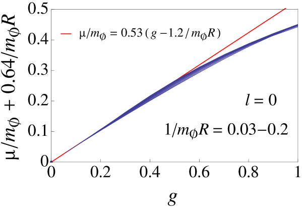
Figure 1: Maximum value of growth rate, $\mu$, shifted by the factor of $0.64/R$ as a function of coupling $g$ for $l=0$, $m_{\chi}=0$, and $1/(m_{\phi}R)=0.03-0.2$. Lines for $1/(m_{\phi}R)=0.03-0.2$ overlap and it is difficult to distinguish among them. We fit the results by the red line for small $g$.

If we neglect the spatial dependence of the I-ball, what we calculate here is a growth rate due to parametric resonance in preheating preheating . In this case, the equation of motion is given by

$$\ddot{\chi}-\nabla^{2}\chi+m_{\chi}^{2}\chi+g\omega_{0}^{2}\cos(\omega_{0}t)\chi=0.$$ (49)

When we consider a fixed Fourier mode of $\chi$, this equation is reduced to the Mathieu equation as

$$\frac{\partial^{2}}{\partial z^{2}}\chi_{k}+\left(A_{k}-2q\cos 2z\right)\chi_{k}=0,$$ (50)

where

$$A_{k} = 4\frac{k^{2}+m_{\chi}^{2}}{\omega_{0}^{2}},$$ (51)

$$q = 2g,$$ (52)

$$z = \frac{\omega_{0}t}{2}+\frac{\pi}{2}.$$ (53)

In the case of $q\lesssim 1$, the resonance occurs in some narrow bands near $A_{k}\simeq 1^{2},2^{2},3^{2},\dots$. The most important instability band is the first one, $A_{k}\simeq 1$, and the maximum growth rate is given by

$$\mu_{0}\simeq gm_{\phi}/2.$$ (54)

The width of the first instability band is of the order of $q$.

The above resonance effect can be interpreted as the collective decay process by Bose stimulation. The elementary decay rate of the field $\phi$ through the interaction of Eq. (21) is calculated as

$$\Gamma_{\phi}=\frac{g^{2}m_{\phi}^{2}}{16\pi\Phi_{0}^{2}}p_{\chi},$$ (55)

where $p_{\chi}=\sqrt{E_{\chi}^{2}-m_{\chi,\text{eff}}^{2}(t)}$ and $E_{\chi}=m_{\phi}/2$. Since the mass of $\chi$ changes with time as $m_{\chi,\text{eff}}(t)^{2}=m_{\chi}^{2}+g\omega_{0}^{2}\cos(\omega_{0}t)$, there is the uncertainty in the momentum of the field $\chi$ which is estimated as

$$\Delta p_{\chi}=\frac{\Delta m_{\chi,\text{eff}}^{2}}{2p_{\chi}}\sim\frac{g\omega_{0}^{2}}{p_{\chi}}.$$ (56)

In order to take the effects of Bose enhancement into account, we need to count the number of states where the $\chi$-particles can occupy. In our case, this can be estimated as

$$\Delta N_{\rm ns} \approx \frac{\Delta^{3}p_{\chi}\Delta^{3}x}{(2\pi)^{3}},$$ (57)

$$\approx \frac{p_{\chi}^{2}\Delta p_{\chi}V}{2\pi^{2}}\approx\frac{g\omega_{0}^{2}p_{\chi}V}{2\pi^{2}},$$

where $V$ is an arbitrary scale of volume. Then, we can estimate the production rate for each state from the decay of condensation $\phi$ as

$$\frac{1}{\Delta N_{\rm ns}}\left(n_{\phi}V\right)2\Gamma_{\phi}\approx\frac{2\pi^{2}}{g\omega_{0}^{2}p_{\chi}V}\left(\frac{1}{2}\omega_{0}\Phi_{0}^{2}V\right)\frac{2g^{2}m_{\phi}^{2}}{16\pi\Phi_{0}^{2}}p_{\chi}\approx\frac{\pi}{8}gm_{\phi},$$ (58)

where we use $\omega_{0}\simeq m_{\phi}$, and $n_{\phi}$ ($=\omega_{0}\Phi_{0}^{2}/2$) is the number density of the field $\phi$. We insert the factor of $2$ because two particles of $\chi$ are produced through each decay of $\phi$. This result is independent from the arbitrary scale of volume $V$, as expected. Since the actual decay rate is proportional to the occupation number in the final state due to Bose stimulation, the number density of particles $\chi$ grows exponentially with the growth rate of $\mu_{0}\approx\pi gm_{\phi}/8$. This result is consistent with Eq. (54) which is derived on the basis of the Mathieu equation.

In the case of the I-ball with finite radius $R$ ($=1/K^{1/2}m_{\phi}$), the particles in the final state escape from the I-ball. Therefore the effects of Bose enhancement are relevant only if the particle production rate is larger than a certain escape rate from the I-ball previous work . The escape rate can be estimated as $v_{\chi}/R$ where $v_{\chi}$ is the velocity of the particle $\chi$, and we can say that the I-ball decay rate is affected by Bose enhancement when $\mu_{0}>\mu_{*}\sim v_{\chi}/R$. In fact, Fig. 1 shows that the growth rate is approximately given by

$$\mu\simeq 0.53m_{\phi}\left(g-\frac{1.2}{m_{\phi}R}\right),$$ (59)

for small $g$ and $m_{\chi}=0$. This indicates that $\mu_{*}\simeq 0.64/R$ for $m_{\chi}=0$. Also, the magnitude of the proportionality constant ($0.53m_{\phi}$) is consistent with the analytic estimation derived above [see Eq. (54) or (58)]. When we define $g^{*}$ as a critical value of the coupling constant above which a non-zero growth rate $\mu$ is obtained, it is given by $g^{*}\simeq 1.2/(m_{\phi}R)$ for $m_{\chi}=0$.

IV.2 Case of $m_{\chi}>0$ and $l=0$

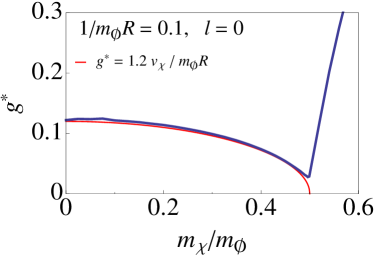
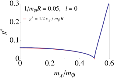
Figure 2: Critical value of the coupling $g^{*}$ as a function of mass $m_{\chi}$ for $l=0$. The inverse of radius is $1/(m_{\phi}R)=0.1$ (left) and $0.05$ (right). We fit the results by red curves in light of $g^{*}\propto v_{\chi}$ for $m_{\chi}\lesssim m_{\phi}/2$. Critical values of the coupling $g^{*}$ reach finite lower bounds for $m_{\chi}\approx m_{\phi}/2$ because of the uncertainty in the momentum estimated in Eq. (56).

Next, we study the effect of a finite mass of $\chi$. Figure 2 shows the mass dependence of $g^{*}$ as

$$g^{*}\propto v_{\chi}=\frac{p_{\chi}}{E_{\chi}}\quad\text{ for }\ m_{\chi}\lesssim\frac{m_{\phi}}{2},$$ (60)

where $p_{\chi}=\sqrt{E_{\chi}^{2}-m_{\chi}^{2}}$ and $E_{\chi}=m_{\phi}/2$. This is consistent with the explanation given in the previous subsection that the escape rate is proportional to the velocity of $\chi$. However, there is a lower bound for the velocity since there is the uncertainty in the momentum of the field $\chi$, which is estimated in Eq. (56). Using Eq. (56) with $p_{\chi}\sim\Delta p_{\chi}$ for $m_{\chi}\approx m_{\phi}/2$, we can estimate the lower bound of the effective velocity as $\text{Min}[v_{\chi}]\sim 2g^{1/2}$. Therefore the critical value of the coupling $g^{*}$ reaches a non-zero lower bound $g^{*}_{min}$ when $m_{\chi}\approx m_{\phi}/2$, where

$$g^{*}_{\text{min}} \sim \frac{\text{Min}[v_{\chi}]}{m_{\phi}R}\sim\frac{2(g^{*}_{\text{min}})^{1/2}}{m_{\phi}R},$$

$$\Leftrightarrow~{}~{}~{}~{}~{}g^{*}_{\text{min}} \sim \frac{4}{(m_{\phi}R)^{2}}.$$ (61)

We thus obtain the analytic estimation for $g^{*}_{\text{min}}$, which can be compared with the result shown in Fig. 2. In fact, the figure indicates that numerically it is given by

$$g^{*}_{\text{min}}\simeq\frac{2}{(m_{\phi}R)^{2}},$$ (62)

which is consistent with Eq (61).

IV.3 Case of $m_{\chi}=0$ and $l>0$

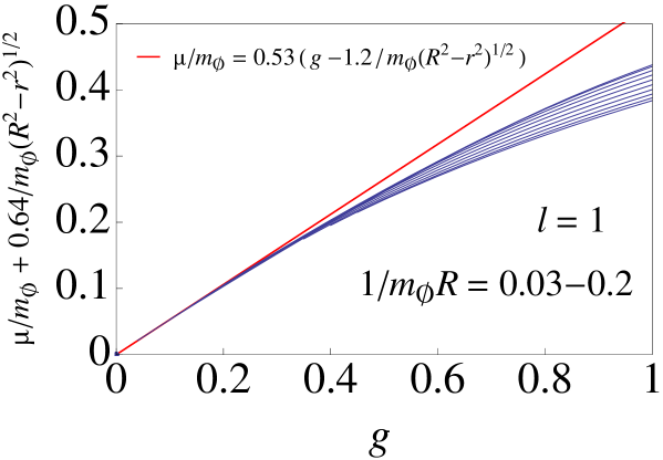
Figure 3: Maximum value of growth rate, $\mu$, shifted by the factor of $0.64/(R^{2}-r^{2})^{1/2}$ as a function of coupling $g$ for $l=1$, $m_{\chi}=0$, and $1/(m_{\phi}R)=0.03-0.2$, where $r=[l(l+1)]^{1/2}/p_{\chi}$. We fit the results by the red line for small $g$.

Let us consider the growth rate when the daughter $\chi$-particle has angular momentum $\ell$. Figure 3 shows that growth rates depend complicatedly on the size of I-ball $R$ for the case of $l=1$. These behaviors are understood by taking the finite-size effect into account. In classical mechanics, the angular momentum of a particle is given by the product of its momentum, $p_{\chi}$, and its position from the origin, $r$. When a particle is produced at some position away from the origin, the distance from that point to the I-ball surface is given by $\sqrt{R^{2}-r^{2}}$ (see Fig. 4). Therefore its escape rate is now given by

$$\frac{v_{\chi}}{m_{\phi}\sqrt{R^{2}-r^{2}}}.$$ (63)

In the case considered here, $r=[l(l+1)]^{1/2}/p_{\chi}$ since the total angular momentum is given by $[l(l+1)]^{1/2}$. Taking these into account, we fit the results in Fig. 3 as

$$g^{*}\simeq\frac{1.2v_{\chi}}{m_{\phi}R\sqrt{1-l(l+1)/(p_{\chi}R)^{2}}}.$$ (64)

Figure 4: Classical description for the motion of $\chi$ produced from I-ball decay. For $l\neq 0$, the daughter particle $\chi$ is produced at a finite distance from the origin, $r$. The distance from that point to the I-ball surface is given by $\sqrt{R^{2}-r^{2}}$.

IV.4 Case of $m_{\chi}>0$ and $l>0$

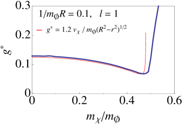
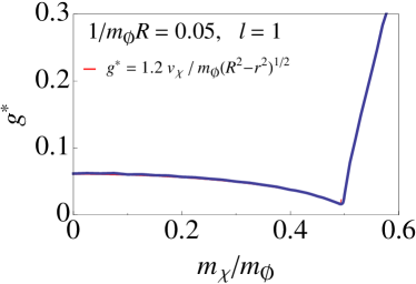
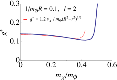
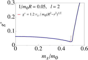
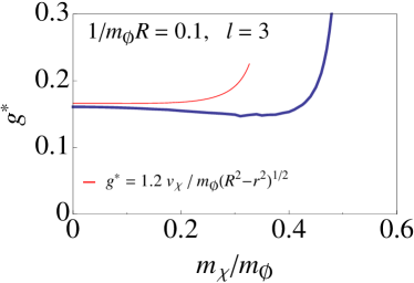
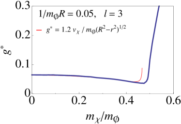
Figure 5: Critical value of the coupling $g^{*}$ as a function of mass $m_{\chi}$ for $l=1$ (top), $2$ (middle), and $3$ (bottom). The inverse of radius is $1/(m_{\phi}R)=0.1$ (left) and $0.05$ (right). Red curves are functions derived analytically as $g^{*}=1.2v_{\chi}/m_{\phi}(R^{2}-r^{2})^{1/2}$. There are gaps between the numerical and analytical results due to the uncertainty in the momentum, which is proportional to the coupling $g$ (see Eq. (56)).

We also calculate the mass dependence of $g^{*}$ for each $l$ ($=1$, $2$, and $3$) as shown in Fig. 5. The results are consistent with Eq. (64) when we take into account the uncertainty in the momentum estimated in Eq. (56). Since $v_{\chi}=p_{\chi}/E_{\chi}$ and $E_{\chi}=m_{\phi}/2$, we can find the lower bound for $g^{*}$ from Eq. (64) by carrying out the differentiation and set it equal to zero. If we neglect the uncertainty in the momentum, we obtain

$$\text{Min}\left[g^{*}\right]=1.2\times\frac{3\sqrt{3l(l+1)}}{(m_{\phi}R)^{2}},$$ (65)

at the momentum of

$$p_{\chi}=\frac{3\sqrt{l(l+1)}}{2R}.$$ (66)

If this momentum is sufficiently larger than the uncertainty in the momentum, the derivation of Eqs. (65) and (66) is consistent. On the other hand, if the momentum of Eq. (66) is less than the uncertainty in the momentum, the lower bound for $g^{*}$ is again determined by Eq. (62). Equation (65) indicates that the lower bound of $g^{*}$ increases with increasing the angular momentum $l$, as we can see in Fig. 5.

V Summary and discussions

Our results calculated in section IV are summarized as follows. If we neglect the uncertainty in the momentum, the growth rate is approximately written as

$$\mu\simeq 0.53m_{\phi}\left(g-g^{*}\right)\qquad\text{ for }g\ll 1,$$ (67)

where $g^{*}$ is given by

$$g^{*}\simeq\frac{1.2v_{\chi}}{m_{\phi}R\sqrt{1-l(l+1)/(p_{\chi}R)^{2}}}.$$ (68)

When $l=0$ and $m_{\chi}\approx m_{\phi}/2$, the uncertainty in the momentum given by Eq. (56) is important and $g^{*}$ approaches the value of

$$g^{*}_{\text{min}}\simeq\frac{2}{(m_{\phi}R)^{2}}.$$ (69)

As apparent from Eq. (68), the critical value is larger for non-zero angular momentum. In other words, the rate of exponential decay with non-zero angular momentum is smaller than the one with zero angular momentum.

Since the decay rate of I-balls grows exponentially as $\sim\exp(\mu t)$, I-balls decay instantaneously at the time of $t\sim\mu^{-1}\sim H^{-1}$, where $H$ is the Hubble parameter. From Eq. (67), the temperature at the I-ball decay, $T_{\text{d}}$, can be calculated as

$$T_{\text{d}} \simeq \left(\frac{90}{4\pi^{2}g_{s}}\right)^{1/4}\sqrt{\mu M_{\text{P}}},$$ (70)

$$\simeq 10^{10}\text{ GeV}\times(g-g^{*})^{1/2}\left(\frac{m_{\phi}}{\text{TeV}}\right)^{1/2},$$

where $g_{s}$ is the effective relativistic degrees of freedom at the decay time. This reheating temperature is larger than the one derived from the perturbative decay rate (55) by the factor of

$$\left(\frac{\mu}{\Gamma_{\phi}}\right)^{1/2}\simeq\left(0.53\frac{g-g^{*}}{g}\frac{16\pi\Phi_{0}^{2}}{gm_{\phi}p_{\chi}}\right)^{1/2},$$ (71)

where we use Eq. (55). This factor is larger for larger I-balls (see Eq. (19)) and for smaller coupling constant. Another important property is that I-balls can decay only into the particle which interacts with the I-balls with a coupling constant larger than $g^{*}$. This property may allow us to obtain a high reheating temperature without producing unwanted relics and may lead to new cosmological scenarios of non-thermal dark matter production and non-thermal leptogenesis.

Finally, we comment on the difference between preheating and I-ball decay. Since the growth rate is proportional to the amplitude of the oscillating field $\Phi_{0}$, it decreases due to the Hubble expansion as $\mu\propto\Phi_{0}\propto a^{-3/2}$ in the case of preheating, where $a$ is the scale factor. On the other hand, since the dynamics of the amplitude of the I-ball $\phi_{0}$ decouples from the Hubble expansion, the growth rate $\mu$ remains constant in time in the case of I-ball decay. Therefore the I-ball eventually decays exponentially when $\mu>0$, i.e., when the coupling of interaction is larger than the critical value of the coupling, $g^{*}$.

VI Conclusions

We have focused on I-balls in the scalar field theory with the monomial potential of $V(\phi)\propto\phi^{2(1-K)}$ and $0<K\ll 1$ in $3+1$ dimensions, which is motivated by chaotic inflationary models and supersymmetric theories. The stability of I-ball is guaranteed by the conservation of an adiabatic invariant, which also determines the configuration of the I-ball as Gaussian in that theory. We have calculated the decay rate of the Gaussian-type I-ball through a interaction with another scalar field, taking into account the effects of Bose enhancement. In Ref. previous work , a non-perturbative method to compute the decay rate has been derived in general dimensions. We have applied the method assuming spherical symmetry and have calculated the partial decay rates into partial waves, labelled by the angular momentum of daughter particles. We have also revealed the conditions that the I-ball decays exponentially.

While the effects of Bose enhancement is proportional to the number density of the daughter particles inside the I-ball, the daughter particles escape from the I-ball. Therefore the effects of Bose enhancement are relevant only if a production rate is larger than a certain escape rate from the I-ball previous work . In other words, there is a critical value of the coupling constant above which the I-ball decays exponentially due to Bose stimulation and below which it decays linearly through elementary decay processes. The critical value is basically proportional to the product of the velocity of daughter particles and the inverse of the size of the I-ball. However, we have to take account of the lower bound of velocity, which comes from an uncertainty in the momentum of daughter particles and is again proportional to the inverse of the size of the I-ball. In the case of non-zero angular momentum for daughter particles, the critical value is larger than the one in the case of zero angular momentum. Therefore, the rate of exponential decay with non-zero angular momentum is smaller than the one with zero angular momentum.

In chaotic inflation models with the above potential, I-balls are in fact formed under some conditions oscillon2011 . In this scenario, inflaton begins to oscillate soon after inflation ends, and then instabilities of the inflaton oscillation grow to form I-balls. Since I-balls still dominate the energy density of the Universe, the decay rate of I-ball determines the reheating temperature of the Universe. If the decay rate of I-ball is enhanced by Bose stimulation, the reheating temperature is much larger than the one derived from the perturbative decay rate. Another important consequence is that I-balls can decay only into the particle which interacts with the I-balls with coupling constants larger than the critical value. These properties may lead to some implications for the physics related to the reheating process of the Universe.

- (1) R. F. Dashen, B. Hasslacher and A. Neveu, Phys. Rev. D 11, 3424 (1975).
- (2) I. L. Bogolyubsky and V. G. Makhankov, JETP Lett. 24, 12 (1976).
- (3) M. Gleiser, Phys. Rev. D 49, 2978 (1994) [hep-ph/9308279].
- (4) E. W. Kolb and I. I. Tkachev, Phys. Rev. D 49, 5040 (1994) [astro-ph/9311037].
- (5) E. J. Copeland, M. Gleiser and H. -R. Muller, Phys. Rev. D 52, 1920 (1995) [hep-ph/9503217].
- (6) P. B. Greene, L. Kofman and A. A. Starobinsky, Nucl. Phys. B 543, 423 (1999) [hep-ph/9808477].
- (7) J. McDonald, Phys. Rev. D 66, 043525 (2002) [hep-ph/0105235].
- (8) S. Kasuya, M. Kawasaki and F. Takahashi, Phys. Lett. B 559, 99 (2003) [hep-ph/0209358].
- (9) M. Broadhead and J. McDonald, Phys. Rev. D 72, 043519 (2005) [hep-ph/0503081].
- (10) P. M. Saffin and A. Tranberg, JHEP 0701, 030 (2007) [hep-th/0610191].
- (11) M. Hindmarsh and P. Salmi, Phys. Rev. D 74, 105005 (2006) [hep-th/0606016].
- (12) G. Fodor, P. Forgacs, P. Grandclement and I. Racz, Phys. Rev. D 74, 124003 (2006) [hep-th/0609023].
- (13) E. Farhi, N. Graham, A. H. Guth, N. Iqbal, R. R. Rosales and N. Stamatopoulos, Phys. Rev. D 77, 085019 (2008) [arXiv:0712.3034 [hep-th]].
- (14) M. Hindmarsh and P. Salmi, Phys. Rev. D 77, 105025 (2008) [arXiv:0712.0614 [hep-th]].
- (15) G. Fodor, P. Forgacs, Z. Horvath and A. Lukacs, Phys. Rev. D 78, 025003 (2008) [arXiv:0802.3525 [hep-th]].
- (16) M. A. Amin and D. Shirokoff, Phys. Rev. D 81, 085045 (2010) [arXiv:1002.3380 [astro-ph.CO]].
- (17) M. Gleiser, N. Graham and N. Stamatopoulos, Phys. Rev. D 82, 043517 (2010) [arXiv:1004.4658 [astro-ph.CO]].
- (18) M. A. Amin, arXiv:1006.3075 [astro-ph.CO].
- (19) M. A. Amin, R. Easther and H. Finkel, JCAP 1012, 001 (2010) [arXiv:1009.2505 [astro-ph.CO]].
- (20) M. Gleiser, N. Graham and N. Stamatopoulos, Phys. Rev. D 83, 096010 (2011) [arXiv:1103.1911 [hep-th]].
- (21) M. A. Amin, R. Easther, H. Finkel, R. Flauger and M. P. Hertzberg, Phys. Rev. Lett. 108, 241302 (2012) [arXiv:1106.3335 [astro-ph.CO]].
- (22) M. Kawasaki and N. Takeda, arXiv:1310.4615 [astro-ph.CO].
- (23) H. Segur and M. D. Kruskal, Phys. Rev. Lett. 58, 747 (1987).
- (24) N. Graham and N. Stamatopoulos, Phys. Lett. B 639, 541 (2006) [hep-th/0604134].
- (25) M. Gleiser and D. Sicilia, Phys. Rev. Lett. 101, 011602 (2008) [arXiv:0804.0791 [hep-th]].
- (26) G. Fodor, P. Forgacs, Z. Horvath and M. Mezei, Phys. Rev. D 79, 065002 (2009) [arXiv:0812.1919 [hep-th]].
- (27) G. Fodor, P. Forgacs, Z. Horvath and M. Mezei, Phys. Lett. B 674, 319 (2009) [arXiv:0903.0953 [hep-th]].
- (28) M. Gleiser and D. Sicilia, Phys. Rev. D 80, 125037 (2009) [arXiv:0910.5922 [hep-th]].
- (29) M. P. Hertzberg, Phys. Rev. D 82, 045022 (2010) [arXiv:1003.3459 [hep-th]].
- (30) P. Salmi and M. Hindmarsh, Phys. Rev. D 85, 085033 (2012) [arXiv:1201.1934 [hep-th]].
- (31) E. Komatsu et al. [WMAP Collaboration], Astrophys. J. Suppl. 192, 18 (2011). [arXiv:1001.4538 [astro-ph.CO]].
- (32) P. A. R. Ade et al. [Planck Collaboration], arXiv:1303.5082 [astro-ph.CO].
- (33) K. Enqvist and J. McDonald, Phys. Lett. B 425, 309 (1998) [hep-ph/9711514]; Nucl. Phys. B 538, 321 (1999) [hep-ph/9803380]; Nucl. Phys. B 570, 407 (2000) [hep-ph/9908316].
- (34) M. Dine, L. Randall and S. D. Thomas, Nucl. Phys. B 458, 291 (1996) [hep-ph/9507453].
- (35) S. Coleman, Nucl. Phys. B262 (1985) 263.
- (36) L. Kofman, A. D. Linde and A. A. Starobinsky, Phys. Rev. D 56, 3258 (1997) [hep-ph/9704452].
- (37) I. Affleck and M. Dine, Nucl. Phys. B 249, 361 (1985).
- (38) M. Kawasaki, K. Kohri and T. Moroi, Phys. Rev. D 71, 083502 (2005) [astro-ph/0408426].
- (39) M. Kawasaki, K. Kohri, T. Moroi and A. Yotsuyanagi, Phys. Rev. D 78, 065011 (2008) [arXiv:0804.3745 [hep-ph]].
- (40) T. Moroi, H. Murayama and M. Yamaguchi, Phys. Lett. B 303, 289 (1993).
- (41) T. Moroi and L. Randall, Nucl. Phys. B 570, 455 (2000) [hep-ph/9906527].
- (42) G. F. Giudice, E. W. Kolb and A. Riotto, Phys. Rev. D 64, 023508 (2001) [hep-ph/0005123].
- (43) T. Asaka, K. Hamaguchi, M. Kawasaki and T. Yanagida, Phys. Lett. B 464, 12 (1999) [hep-ph/9906366].
- (44) A. Kusenko, Phys. Lett. B 404, 285 (1997) [hep-th/9704073]; Phys. Lett. B 405, 108 (1997) [hep-ph/9704273].
- (45) A. Kusenko and M. E. Shaposhnikov, Phys. Lett. B 418, 46 (1998). [hep-ph/9709492].
- (46) S. Kasuya and M. Kawasaki, Phys. Rev. D 61, 041301(R) (2000) [hep-ph/9909509]; Phys. Rev. D 62, 023512 (2000). [hep-ph/0002285]; Phys. Rev. D 64, 123515 (2001). [hep-ph/0106119].
- (47) K. Mukaida and K. Nakayama, JCAP 1301, 017 (2013) [JCAP 1301, 017 (2013)] [arXiv:1208.3399 [hep-ph]].
- (48) T. Hiramatsu, M. Kawasaki and F. Takahashi, JCAP 1006, 008 (2010). [arXiv:1003.1779 [hep-ph]].
- (49) A. G. Cohen, S. R. Coleman, H. Georgi and A. Manohar, Nucl. Phys. B 272, 301 (1986).
- (50) A. Kusenko, L. Loveridge and M. Shaposhnikov, Phys. Rev. D 72, 025015 (2005) [hep-ph/0405044].
- (51) M. Kawasaki and M. Yamada, Phys. Rev. D 87, 023517 (2013) [arXiv:1209.5781 [hep-ph]].