The Asymptotic Size of The Largest Component in Random Geometric Graphs with some applications

Abstract

For the size of the largest component in a supercritical random geometric graph, this paper estimates its expectation which tends to a polynomial on a rate of exponential decay, and sharpens its asymptotic result with a central limit theory. Similar results can be obtained for the size of biggest open cluster, and for the number of open clusters of percolation on a box, and so on.

Ge Chen, Changlong Yao and Tiande Guo

Ge Chen National Center for Mathematics and Interdisciplinary Sciences & Key Laboratory of Systems and Control, Academy of Mathematics and Systems Science, Chinese Academy of Sciences, Beijing, 100190, P.R.China. Email: chenge@amss.ac.cn. [Academy of Mathematics and Systems Science, CAS]Changlong Yao Institute of Applied Mathematics, Academy of Mathematics and Systems Science, Chinese Academy of Sciences, Beijing, 100190, P.R.China. Email: deducemath@126.com. [Graduate University of Chinese Academy of Sciences]Tiande Guo School of Mathematical Science, Graduate University of Chinese Academy of Sciences, Beijing, 100049, P.R.China. Email: tdguo@gucas.ac.cn.

60K3560D05;82B43;

1 Introduction

The size of the largest component is a basic property for random geometric graphs (RGGs) and has attracted much interest during the past years, including both theoretical studies [7][10][8][9] and various applications [1][3][12][11]. This paper firstly investigates the asymptotic size of the largest component of RGG in the supercritical case.

Given a set $\mathcal{X}\subset\mathbb{R}^{d}$, let $G(\mathcal{X};r)$ denote the undirected graph with vertex set $\mathcal{X}$ and with undirected edges which connect all those pairs $\{X,Y\}$ with $\parallel Y-X\parallel\leq r$, where $\|\cdot\|$ denotes the Euclidean norm ($l_{2}-norm$). The basic model of RGGs can be formulated as $G(\mathcal{X}_{n};r_{n})$, where $\mathcal{X}_{n}$ denotes $n$ points which are independently and uniformly distributed in a $d$-dimensional unit cube. To overcome the lack of spatial independence for the binomial point process $\mathcal{X}_{n}$, the model of continuum percolation must be introduced. Following Section 1.7 in [9], let $\mathcal{H}_{\lambda}$ be a homogeneous Poisson process of intensity $\lambda$ on $\mathbb{R}^{d}$. For $s>0$, define $B(s):=[0,s]^{d}$ and $\mathcal{H}_{\lambda,s}:=\mathcal{H}_{\lambda}\cap B(s).$ Following [9], we write the Poisson Boolean model as $G(\mathcal{H}_{\lambda,s};1)$.

There exist some notations related to percolation must be introduced. Following Section 9.6 in [9], let $\mathcal{H}_{\lambda,0}$ denote the point process $\mathcal{H}_{\lambda}\cup\{\textbf{0}\}$, where 0 is the origin in $\mathbb{R}^{d}$, and for $k\in\mathds{N}$, let $p_{k}(\lambda)$ denote the probability that the order of the component in $G(\mathcal{H}_{\lambda,0};1)$ containing the origin is equal to $k$. The $percolation$ $probability$ $p_{\infty}(\lambda)$ is defined to be the probability that 0 lies in an infinite component of the graph $G(\mathcal{H}_{\lambda,0};1)$. Therefore, we have $p_{\infty}(\lambda)=1-\sum\limits_{k=1}^{\infty}p_{k}(\lambda)$. Let

$$\lambda_{c}=inf\{\lambda>0:p_{\infty}(\lambda)>0\}$$ (1)

denote the critical intensity of continuum percolation. It is well known that $0<\lambda_{c}<\infty$ for $d\geq 2$ [4][2][6].

Following Section 9.6 in [9], let $L_{j}(G)$ denote the order of its $j$th-largest component for any graph $G$. Then $L_{1}(G(\mathcal{H}_{\lambda,s};1))$ denotes the order of the largest component of $G(\mathcal{H}_{\lambda,s};1)$. The asymptotic properties of $L_{1}(G(\mathcal{H}_{\lambda,s};1))$ have been well studied by Penrose. The basic asymptotic result about $L_{1}(G(\mathcal{H}_{\lambda,s};1))$ is provided by Penrose (Theorem 10.9 in [9]), that if $\lambda\neq\lambda_{c}$ then

$$s^{-d}L_{1}(G(\mathcal{H}_{\lambda,s};1))\xrightarrow{P}\lambda p_{\infty}(\lambda)\quad as\quad s\rightarrow\infty.$$ (2)

Also, Penrose has given a central limit theorem for $L_{1}(G(\mathcal{H}_{\lambda,s};1))$ in the supercritical case $\lambda>\lambda_{c}$ (Theorem 10.22 in [9]), that

$$s^{-d/2}(L_{1}(G(\mathcal{H}_{\lambda,s};1))-E[L_{1}(G(\mathcal{H}_{\lambda,s};1))])\xrightarrow{D}\mathcal{N}(0,\sigma^{2}).$$ (3)

However, the question as how large $E[L_{1}(G(\mathcal{H}_{\lambda,s};1))]$ should be still remains unsolved. By (2) it can be deduced that $E[L_{1}(G(\mathcal{H}_{\lambda,s};1))]=\lambda p_{\infty}(\lambda)s^{d}+o(s^{d})$, where $f(s)=o(g(s))$ indicates that $\lim_{s\rightarrow\infty}\frac{f(s)}{g(s)}=0$. This result is not precise enough for some theoretic analysis and practical applications.

The corresponding asymptotic results and central limit theorem for $G(\mathcal{X}_{n};r_{n})$ have also been established by Peorose (Theorems 11.9 and 11.16 in [9]), but we may ask similar questions. This paper will study the problem and give a more precise description for the asymptotic sizes of $L_{1}(G(\mathcal{H}_{\lambda,s};1))$ and $L_{1}(G(\mathcal{X}_{n};r_{n}))$. Our method can be adapted to study some other models and problems.

2 Main Results

Our main results can be formulated as the following two theorems.

Theorem 1

Suppose $d\geq 2$ and $\lambda>\lambda_{c}$. Then there exist constants $c=c(d,\lambda)>0$ and $\tau_{i}=\tau_{i}(d,\lambda)$, $1\leq i\leq d$, with $\tau_{1}>0$, such that for all $s$ large enough,

$$E[L_{1}(G(\mathcal{H}_{\lambda,s};1))]=\lambda p_{\infty}(\lambda)s^{d}-\sum_{i=1}^{d}\tau_{i}s^{d-i}+o\left(e^{-cs}\right).$$ (4)

Also, there exists a constant $\sigma=\sigma(d,\lambda)>0$, such that

$$L_{1}(G(\mathcal{H}_{\lambda,s};1))s^{-d/2}-\lambda p_{\infty}(\lambda)s^{d/2}+\sum_{i=1}^{\lfloor\frac{d}{2}\rfloor}\tau_{i}s^{d/2-i}\xrightarrow{D}\mathcal{N}(0,\sigma^{2})$$ (5)

as $s\rightarrow\infty$.

Theorem 2

Suppose $d\geq 2$ and $\lambda>\lambda_{c}$. Let $\sigma$ and $\tau_{i}$ be the same constants appearing in Theorem 1. There exists a constant $\delta=\delta(d,\lambda)$, with $0<\delta\leq\sigma$, such that

$$L_{1}\left(G\left(\mathcal{X}_{n};(n/\lambda)^{-1/d}\right)\right)\left(n/\lambda\right)^{-1/2}-p_{\infty}(\lambda)\left(\lambda n\right)^{1/2}+\sum_{i=1}^{\lfloor\frac{d}{2}\rfloor}\tau_{i}\left(n/\lambda\right)^{\frac{1}{2}-\frac{i}{d}}\xrightarrow{D}\mathcal{N}(0,\delta^{2})$$

as $n\rightarrow\infty$.

To prove the two theorems, we estimate the value of $E[L_{1}(G(\mathcal{H}_{\lambda,s};1))]$ firstly, and then using the central limit theorems for $L_{1}(G(\mathcal{H}_{\lambda,s};1))$ and $L_{1}(G(\mathcal{X}_{n};(n/\lambda)^{-1/d}))$, we can prove (5) and Theorem 2.

Some notations must be stated before the proof of our results. For any $x\in\mathbb{R}^{d}$, we write its $l_{\infty}$ norm with $\|x\|_{\infty}$ given by the maximum absolute value of its coordinates. For any finite set $A\subset\mathbb{R}^{d}$, we set the diameter of $A$ by diam$(A)=\sup_{x,y\in A}\|x-y\|_{\infty}.$ Also, let $|A|$ denote the cardinality of $A$.

Let $\oplus$ denote the Minkowski addition of sets. Let $Leb(\cdot)$ denote the Lebesgue measure. For $s\geq 0$, let $\lfloor s\rfloor$ denote the smallest integer not smaller than $s$.

To simplify the expression, we will omit the dependence of all constants on $d$ and $\lambda$, for example, the constant $c$ stands for $c(d,\lambda)$.

Given $\lambda>\lambda_{c}$, by the uniqueness of the infinite component in continuum percolation (Theorem 9.19 in [9]), the infinite graph $G(\mathcal{H}_{\lambda};1)$ has precisely one infinite component $\mathcal{C}_{\infty}$ with probability $1$. Let $C_{1},C_{2},...,C_{M}$ denote the components of $G(\mathcal{C}_{\infty}\cap B(s);1)$, taken in a decreasing order. We give a result on the rate of sub-exponential decay of the difference between $E[L_{1}(G(\mathcal{H}_{\lambda,s};1))]$ and $E[|C_{1}|]$.

Lemma 3

Suppose $d\geq 2$ and $\lambda>\lambda_{c}$. The exists a constant $c>0$, such that for large enough $s$,

$$0\leq E[L_{1}(G(\mathcal{H}_{\lambda,s};1))]-E[|C_{1}|]\leq e^{-cs}.$$ (6)

Proof 2.1

By the definition of $L_{1}(G(\mathcal{H}_{\lambda,s};1))$ and $C_{1}$, obviously $E[L_{1}(G(\mathcal{H}_{\lambda,s};1))]\geq E[|C_{1}|]$. Thus it just remains to prove the second inequality of (6).

Given any $x\in\mathbb{R}^{d}$, let $C_{\infty}(x)$ denote the infinite connected component of $G(\mathcal{H}_{\lambda}\cup\{x\};1)$. By Palm theorem for Poisson processes (Theorem 1.6 in [9]), we have

$$E[L_{1}(G(\mathcal{H}_{\lambda,s};1))]=\lambda\int_{B(s)}P[x\in V_{1}(x)]dx,$$

where $V_{1}(x)$ denotes the largest component of $G(\mathcal{H}_{\lambda,s}\cup\{x\};1)$, and

$$E[|C_{1}|]=\lambda\int_{B(s)}P[x\in C_{1}(x)]dx,$$

where $C_{1}(x)$ denotes the largest component of $C_{\infty}(x)\cap B(s)$. Therefore,

$$\begin{aligned} E[L_{1}(G(\mathcal{H}_{\lambda,s};1))]-E[|C_{1}|]&=\lambda\int_{B(s)}(P[x\in V_{1}(x)]-P[x\in C_{1}(x)])dx\\ &\leq\lambda\int_{B(s)}P[\{x\in V_{1}(x)\}\cap\{x\notin C_{1}(x)\}]dx\\ &=\lambda\int_{B(s)}P[\{x\in V_{1}(x)\}\cap\{x\notin C_{\infty}(x)\}]dx.\end{aligned}$$ (7)

Suppose $0<\varepsilon<\frac{1}{2}$. By Theorem 10.19 in [9], there exist constants $c_{1}>0$ and $s_{1}>0$, such that if $s>s_{1}$ then

$$\begin{aligned} P\left[|V_{1}(x)|<(1-\varepsilon)\lambda s^{d}p_{\infty}(\lambda)\right]&\leq P\left[L_{1}(G(\mathcal{H}_{\lambda,s};1))<(1-\varepsilon)\lambda s^{d}p_{\infty}(\lambda)\right]\\ &\leq\exp\left(-c_{1}s^{d-1}\right).\end{aligned}$$ (8)

Also, by Theorem 10.15 in [9], there exists a constant $c_{2}>0$ such that for $s$ large enough,

$$\sum\limits_{k\geq\lceil(1-\varepsilon)\lambda s^{d}p_{\infty}(\lambda)\rceil}p_{k}(\lambda)<\exp\left(-c_{2}[(1-\varepsilon)\lambda s^{d}p_{\infty}(\lambda)]^{(d-1)/d}\right).$$ (9)

Therefore, from (8) and (9) we can obtain

$$P[\{x\in V_{1}(x)\}\cap\{x\not\in C_{\infty}(x)\}]$$

$$~{}~{}~{}~{}\leq P[|V_{1}(x)|<(1-\varepsilon)\lambda s^{d}p_{\infty}(\lambda)]$$

$$~{}~{}~{}~{}~{}~{}~{}~{}~{}+P[\{x\in V_{1}(x)\}\cap\{x\not\in C_{\infty}(x)\}\cap\{|V_{1}(x)|\geq(1-\varepsilon)\lambda s^{d}p_{\infty}(\lambda)\}]$$

$$~{}~{}~{}~{}\leq\exp\left(-c_{1}s^{d-1}\right)+\sum\limits_{k\geq\lceil(1-\varepsilon)\lambda s^{d}p_{\infty}(\lambda)\rceil}p_{k}(\lambda)$$

$$~{}~{}~{}~{}<\exp\left(-c_{1}s^{d-1}\right)+\exp\left(-c_{2}[(1-\varepsilon)\lambda p_{\infty}(\lambda)]^{(d-1)/d}s^{d-1}\right)~{}~{}as~{}s\rightarrow\infty.$$

Combined with (7) this yields our result.

To estimate the value of $E[L_{1}(G(\mathcal{H}_{\lambda,s};1))]$, by Lemma 3 we just need to get the value of $E[|C_{1}|]$ instead. Actually, by Palm theory for infinite Poisson process (Theorem 9.22 in [9]),

$$E\left[\sum_{i=1}^{M}|C_{i}|\right]=E[\left|\mathcal{C}_{\infty}\cap B(s)\right|]=\lambda p_{\infty}(\lambda)s^{d},$$ (10)

so we just need to estimate the value of $E[\sum_{i=2}^{M}|C_{i}|]$. Let $L(s):=B(s)\backslash[1,s-1]^{d}$. For any $2\leq i\leq M$, since $C_{i}\subset\mathcal{C}_{\infty}$, therefore there exists at least one point in $L(s)\cap C_{i}$ which connects to $\mathcal{C}_{\infty}\setminus B(s)$ directly; we choose the nearest one to the boundary of $B(s)$ as the $out-connect$ $point$. We can see that each component of $C_{2},...,C_{M}$ contains exactly one out-connect point.

For any region $R\subseteq B(s)$ and $2\leq i\leq M$, define

$$\chi_{i}(R):=\left\{\begin{array}[]{ll}1,&\mbox{if the out-connect point of $C_{i}$ is contained by }R,\\ 0,&\mbox{otherwise},\end{array}\right.$$ (11)

and define

$$\xi(R)=\xi(R,s):=\sum\limits_{i=2}^{M}\chi_{i}(R)|C_{i}|.$$ (12)

By the definition of $\xi(\cdot)$, it is easy to see that for any $R,\widetilde{R}\subset B(s)$, if $Leb(R\cap\widetilde{R})=0$, then $E[\xi(R\cap\widetilde{R})]=0$ and $E[\xi(R\cup\widetilde{R})]=E[\xi(R)]+E[\xi(\widetilde{R})].$

For $0\leq i\leq d-1$, define

$$R_{i}=R_{i}(s):=[0,1]\times\underbrace{[0,s/2]\times\cdots\times[0,s/2]}\limits_{d-1-i}\times\underbrace{[1,s/2]\times\cdots\times[1,s/2]}\limits_{i}.$$

Noted that $[1,s/2]^{d}\cap L(s)=\emptyset$, then by symmetry,

$$\begin{aligned} &E\left[\sum\limits_{i=2}^{M}|C_{i}|\right]=E\left[\xi(B(s))\right]=2^{d}E\left[\xi\left(\left[0,\frac{s}{2}\right]^{d}\right)\right]\\ &=2^{d}\left\{E\left[\xi(R_{0})\right]+E\left[\xi\left(\left[1,\frac{s}{2}\right]\times\left[0,\frac{s}{2}\right]^{d-1}\right)\right]\right\}=2^{d}\sum\limits_{i=0}^{d-1}E\left[\xi(R_{i})\right].\end{aligned}$$ (13)

Thus, we just need to estimate the value of $E\left[\xi\left(R_{i}\right)\right]$. The following Lemmas 4-7 are introduced to get the desired estimation.

Lemma 4

Suppose $d\geq 2$ and $\lambda>\lambda_{c}$. Let $V_{x}=V_{x}(s)$ denote the connected component containing $x$ of $G(\mathcal{H}_{\lambda,s}\cup\{x\};1)$. There exist constants $c>0$ and $n_{0}>0$, such that if $n>n_{0}$ and $s>2n$ then for any point $x\in B(s)$,

$$P\left[n\leq\mbox{diam}(V_{x})\leq s/2\right]<e^{-cn},$$ (14)

and

$$P\left[\left\{|V_{x}|\geq n\right\}\cap\left\{\mbox{diam}(V_{x})\leq s/2\right\}\right]<\exp\left(-cn^{(d-1)/d}\right).$$ (15)

Proof 2.2

The proof uses ideas from the latter part of the proof of Theorem 10.18 in [9]. Given $x\in\mathbb{R}^{d}$, let $\widetilde{z}$ denote the point in $B_{\mathbb{Z}}^{\prime}(n(s))$ satisfying $x\in B_{\widetilde{z}}$, where the definition of $B_{\mathbb{Z}}^{\prime}(n(s))$ and $B_{\widetilde{z}}$ is given in pp.216 and pp.217 of [9] respectively. Also, $C_{x}$, $D_{ext}C_{x}$, $M_{0}$, $n(s)$ and $M(s)$ are defined as same as those appearing in pp.218-219 of [9]. Penrose has proved that $D_{ext}C_{x}$ is $*-$connected and if $|C_{x}|<n(s)^{d}/2$ then

$$\begin{aligned} |D_{ext}C_{x}|\geq(2d)^{-1}(1-({\textstyle\frac{2}{3}})^{1/d})|C_{x}|^{(d-1)/d},\end{aligned}$$ (16)

see pp.219 of [9].

Let $\mathcal{A}_{m,s}$ denote the collection of $*-$connected subsets of cardinality $m$ which disconnects the point $\widetilde{z}$ from the giant component of $B_{\mathbb{Z}}^{\prime}(n(s))$. Then $\mathcal{A}_{m,s}$ is restricted by the box of $B_{\mathbb{Z}}^{\prime}(n(s))\cap([-m,m]^{d}\oplus\widetilde{z})$ and $D_{ext}C_{x}\in\mathcal{A}_{|D_{ext}C_{x}|,s}$. By a Peierls argument (Corollary 9.4 in [9]), the cardinality $|\mathcal{A}_{m,s}|$ is bounded by $(2m+1)^{d}\gamma^{m}$, with $\gamma:=2^{3^{d}}$. Therefore, there exists a constant $k_{0}$ such that for any integer $k>k_{0}$,

$$\begin{aligned} P\left[|D_{ext}C_{x}|\geq k\right]&\leq P\left[\bigcup\limits_{m\geq k}\bigcup\limits_{\sigma\in\mathcal{A}_{m,s}}\{X_{z}=0,\forall z\in\sigma\}\right]\\ &\leq\sum\limits_{m\geq k}(2m+1)^{d}\gamma^{m}(1-p_{1})^{m}<(\frac{2}{3})^{k}.\end{aligned}$$ (17)

By the definition of $C_{x}$ and $D_{ext}C_{x}$, if $n\leq$diam$(V_{x})\leq s/2$ then

$$\frac{n}{M(s)}-1\leq\mbox{diam}(C_{x})\leq\frac{n(s)}{2}+2,$$

and therefore we can get $|C_{x}|<n(s)^{d}/2$ and $|D_{ext}C_{x}|\geq\frac{n}{M(s)}-1$ for large $s$. Therefore, by (17), there exists a constant $n_{0}>0$, such that if $n>n_{0}$ then,

$$P\left[n\leq\mbox{diam}(V_{x})\leq\frac{s}{2}\right]\leq P\left[|D_{ext}C_{x}|\geq\frac{n}{M(s)}-1\right]<\left(\frac{2}{3}\right)^{\frac{n}{2M_{0}}-1}.$$

This yields (14).

It remains to consider the case of $|V_{x}|>n$. Since $C_{x}$ is a $*-$connected component containing $\widetilde{z}$ in $B_{\mathbb{Z}}^{\prime}(n(s))$, by a Peierls argument (Lemma 9.3 in [9]), for all $k$, the number of $*-$ connected subsets of $B_{\mathbb{Z}}^{\prime}(n(s))$ of cardinality $k$ containing $\widetilde{z}$ is at most $\gamma^{k}$. Let $c_{2}\geq e^{2}(2M_{0})^{d}\lambda$. If $|C_{x}|<k$ and $|V_{x}|\geq c_{2}k+1$, then for at least one of these subsets of $B_{\mathbb{Z}}^{\prime}(n(s))$ the union of the associated boxes $B_{z}$ contains at least $c_{2}k$ points of $\mathcal{H}_{\lambda}$. Therefore, by Lemma 1.2 in [9], we have

$$\begin{aligned} P[\{|C_{x}|<k\}\cap\{|V_{x}|\geq c_{2}k+1\}]&<\gamma^{k}P\left[Po\left(k(2M_{0})^{d}\lambda\right)\geq c_{2}k\right]\\ &\leq\gamma^{k}\exp\left\{-\left(\frac{c_{2}k}{2}\right)\log\left(\frac{c_{2}}{(2M_{0})^{d}\lambda}\right)\right\}.\end{aligned}$$ (18)

So if $c_{2}$ is chosen large enough, this probability decays exponentially in $k$.

Set $\beta:=(2d)^{-1}(1-(\frac{2}{3})^{1/d})$. By (16) and (17), we have

$$P[\{\mbox{diam}(V_{x})\leq s/2\}\cap\{|C_{x}|\geq k\}]\leq P\left[|D_{ext}C_{x}|\geq\beta k^{(d-1)/d}\right]<(\frac{2}{3})^{\beta k^{(d-1)/d}}.$$

Combined with (18), this gives (15).

For $x\in B(s)$ and $0<a\leq 1$, define the box

$$B_{i}(x,a):=x\oplus\big{(}\underbrace{[0,1]\times\cdots\times[0,1]}\limits_{i}\times\underbrace{[0,a]\times\cdots\times[0,a]}\limits_{d-i}\big{)}.$$

Also, for any region $R\subseteq B(s)$, define

$$D(R)=D(R,s):=\max_{2\leq j\leq M,\chi_{j}(R)=1}\mbox{diam}(C_{j}).$$

Lemma 5

Suppose $d\geq 2$ and $\lambda>\lambda_{c}$. There exist constants $c>0$ and $n_{0}>0$, such that if $x\in B(s)$, $a\in(0,1]$ and $n>n_{0}$ then

$$P[D(B_{i}(x,a))\geq n]<e^{-cn},$$ (19)

and

$$P[\xi(B_{i}(x,a))\geq n]<\exp\left(-cn^{(d-1)/d}\right)+e^{-cs}.$$ (20)

Proof 2.3

Let $W_{1}$ denote the number of the connected components which intersect with $B_{i}(x,a)$, and have metric diameter not greater than $s/2$ but not smaller than $n$. By Markov’s inequality,

$$P\left[\left\{D(B_{i}(x,a))\geq n\right\}\cap\left\{D(B_{i}(x,a))\leq s/2\right\}\right]\leq P[W_{1}>0]\leq E[W_{1}].$$ (21)

By Palm theory for Poisson process and Lemma 4, if $n>n_{0}$ then

$$\begin{aligned} E[W_{1}]&=\lambda\int_{B_{i}(x,a)}P\left[\left\{\mbox{diam}(V_{x}(s))\geq n\right\}\cap\left\{\mbox{diam}(V_{x}(s))\leq s/2\right\}\right]dx\\ &<\lambda a^{d-i}e^{-cn}.\end{aligned}$$ (22)

Also, $C_{i}$ ($2\leq i\leq M$) is not the largest component of $G(\mathcal{H}_{\lambda,s};1)$, then by Proposition 10.13 in [9], there exist constants $c_{1}>0$ and $s_{1}>0$, such that if $s>s_{1}$ then

$$P\left[D(B_{i}(x,a))>s/2\right]<e^{-c_{1}s}.$$ (23)

Together with (21), (22) and (23), we obtain

$$P[D(B_{i}(x,a))\geq n]<e^{-cn}+e^{-c_{1}s}.$$

Since $P[D(B_{i}(x,a))>s]=0$, thus (19) follows.

Note that $B_{i}(x,a)$ contains at most $2^{d}$ connected components. Thus, if $\xi(B_{i}(x,a))\geq n$, by the definition of $\xi(\cdot)$, there exists at least one component intersecting with $B_{i}(x,a)$ such that it contains no less than $2^{-d}n$ points. Let $W_{2}$ be the number of the connected components which intersect with $B_{i}(x,a)$, and have more than $2^{-d}n$ elements and not larger than $s/2$ metric diameter. With the similar argument as (21) and (22), we get if $n>n_{0}$ then

$$P\left[\left\{\xi(B_{i}(x,a))\geq n\right\}\cap\left\{D(B_{i}(x,a))\leq s/2\right\}\right]\leq E[W_{2}]$$

$$~{}~{}=\lambda\int_{B_{i}(x,a)}P\left[\left\{|V_{x}(s)|\geq 2^{-d}n\right\}\cap\left\{\mbox{diam}(V_{x}(s))\leq s/2\right\}\right]dx$$

$$~{}~{}<\lambda a^{d-i}\exp\left(-c2^{-d}n\right),$$

together with (23) this gives (20).

Let real numbers $s_{1}>2$ and $s_{2}>2$ be given. Let points $x=(x_{1},x_{2},\ldots,x_{d})\in[0,s_{1}/2]^{d}$ and $\widetilde{x}=(\widetilde{x}_{1},\widetilde{x}_{2},\ldots,\widetilde{x}_{d})\in[0,s_{2}/2]^{d}$ be given. For all $1\leq j\leq d$, define

$$N_{x,\widetilde{x}}^{j}(s_{1},s_{2}):=\left\{\begin{array}[]{ll}\min(s_{1},s_{2})-x_{j}-1,&\mbox{if }x_{j}=\widetilde{x}_{j},\\ \min(x_{j},\widetilde{x}_{j},s_{1}-x_{j}-1,s_{2}-\widetilde{x}_{j}-1),&\mbox{otherwise},\end{array}\right.$$

and let

$$N_{x,\widetilde{x}}(s_{1},s_{2}):=\min_{1\leq j\leq d}\lfloor N_{x,\widetilde{x}}^{j}(s_{1},s_{2})\rfloor.$$ (25)

Lemma 6

Let us assume $d\geq 2$, $\lambda>\lambda_{c}$, $1\leq i\leq d$ and $0<a\leq 1$. There exist constants $c>0$ and $n_{0}>0$, such that if $x\in[0,s_{1}/2]^{d}$, $\widetilde{x}\in[0,s_{2}/2]^{d}$ and $N_{x,\widetilde{x}}(s_{1},s_{2})>n_{0}$ then

$$\left|E\left[\xi(B_{i}(x,a),s_{1})\right]-E\left[\xi(B_{i}(\widetilde{x},a),s_{2})\right]\right|<\exp\left(-cN_{x,\widetilde{x}}(s_{1},s_{2})\right).$$

Proof 2.4

Let $B^{\prime}(s_{2}):=B(s_{2})\oplus\{x-\widetilde{x}\},$ and let $\widetilde{C}_{1},\widetilde{C}_{2},\ldots,\widetilde{C}_{\widetilde{M}}$ denote the components of $G(\mathcal{C}_{\infty}\cap B^{\prime}(s_{2});1),$ taking in order of decreasing order. For any region $R\subseteq B^{\prime}(s_{2})$ and $2\leq i\leq\widetilde{M}$, define

$$\widetilde{\chi_{i}}(R):=\left\{\begin{array}[]{ll}1,&\mbox{if the out-connect point of $\widetilde{C}_{i}$ is contained by }R,\\ 0,&\mbox{otherwise}.\end{array}\right.$$

Let $\widetilde{\xi}(R,s_{2}):=\sum_{i=2}^{\widetilde{M}}\widetilde{\chi}_{i}(R)|\widetilde{C}_{i}|$ and define

$$\widetilde{D}(R,s_{2}):=\max_{2\leq j\leq\widetilde{M},\widetilde{\chi}_{j}(R)=1}\mbox{diam}(\widetilde{C}_{j}).$$

According to the ergodicity of Poisson point processes, we can get

$$P\left[\widetilde{\xi}\left(B_{i}(x,a),s_{2}\right)=k\right]=P\left[\xi\left(B_{i}(\widetilde{x},a),s_{2}\right)=k\right],~{}~{}~{}~{}\forall~{}k\geq 1.$$ (26)

Figure 1: If $C_{k}$ connects with $\mathcal{H}_{\lambda}\cap\Delta$, the event of $\xi(B_{i}(x,a),s_{1})\neq\widetilde{\xi}(B_{i}(x,a),s_{2})$ may happen.

Let $\Delta:=B(s_{1})\cup B^{\prime}(s_{2})-B(s_{1})\cap B^{\prime}(s_{2}).$ If $\xi(B_{i}(x,a),s_{1})\neq\widetilde{\xi}(B_{i}(x,a),s_{2})$, then there exists at least one component among $C_{2},\ldots,C_{M},\widetilde{C}_{2},\ldots,\widetilde{C}_{\widetilde{M}}$ which connects directly with $\mathcal{H}_{\lambda}\cap\Delta$, see Figure 1. For simplicity of exposition, we take $N=N_{x,\widetilde{x}}(s_{1},s_{2})$, $\xi_{1}=\xi(B_{i}(x,a),s_{1})$ and $\xi_{2}=\widetilde{\xi}(B_{i}(x,a),s_{2})$. Therefore, by (19), if $N>n_{0}+1$ then

$$\begin{aligned} P\left[\xi_{1}\neq\xi_{2}\right]&\leq P\left[\left\{D(B_{i}(x,a),s_{1})\geq N-1\right\}\cup\left\{\widetilde{D}(B_{i}(x,a),s_{2})\geq N-1\right\}\right]\\ &<2e^{-c(N-1)}.\end{aligned}$$ (27)

Also,

$$\begin{aligned} &P\left[\left\{\xi_{1}=k\right\}\cap\left\{\xi_{2}\neq k\right\}\right]+P\left[\left\{\xi_{1}\neq k\right\}\cap\left\{\xi_{2}=k\right\}\right]\\ &~{}~{}=P\left[\left\{\xi_{1}=k\right\}\right]+P\left[\left\{\xi_{2}=k\right\}\right]-2P\left[\left\{\xi_{1}=k\right\}\cap\left\{\xi_{2}=k\right\}\right]\\ &~{}~{}\geq|P\left[\left\{\xi_{1}=k\right\}\right]-P\left[\left\{\xi_{2}=k\right\}\right]|,\end{aligned}$$ (28)

so by (27) and (28) we have

$$\begin{aligned} &\sum_{k=1}^{\infty}\left|P\left[\left\{\xi_{1}=k\right\}\right]-P\left[\left\{\xi_{2}=k\right\}\right]\right|\\ &~{}~{}\leq\sum_{k=1}^{\infty}\left(P\left[\left\{\xi_{1}=k\right\}\cap\left\{\xi_{1}\neq\xi_{2}\right\}\right]+P\left[\left\{\xi_{2}=k\right\}\cap\left\{\xi_{1}\neq\xi_{2}\right\}\right]\right)\\ &~{}~{}=P\left[\left\{\xi_{1}\geq 1\right\}\cap\left\{\xi_{1}\neq\xi_{2}\right\}\right]+P\left[\left\{\xi_{2}\geq 1\right\}\cap\left\{\xi_{1}\neq\xi_{2}\right\}\right]<4e^{-c(N-1)}.\end{aligned}$$ (29)

Thus, by (26) and (29) we can get

$$\begin{aligned} &\left|E\left[\xi_{1}\right]-E\left[\xi(B_{i}(\widetilde{x},a),s_{2})\right]\right|=\left|\sum_{n=1}^{\infty}\sum_{k=n}^{\infty}\left(P\left[\xi_{1}=k\right]-P\left[\xi_{2}=k\right]\right)\right|\\ &<4N^{d/(d-1)}e^{-c(N-1)}+\sum_{n=N^{d/(d-1)}}^{\infty}\left(P\left[\xi_{1}\geq n\right]+P\left[\xi_{2}\geq n)\right]\right).\end{aligned}$$ (30)

In the following we estimate the upper bound of $\sum_{n=N^{d/(d-1)}}^{\infty}P[\xi_{1}\geq n]$. Firstly, by (20), for $N$ large enough, we can obtain

$$\begin{aligned} \sum\limits_{n=N^{d/(d-1)}}^{e^{2}\lambda s_{1}^{d}}P[\xi_{1}\geq n]<\sum\limits_{n=N^{d/(d-1)}}^{e^{2}\lambda s_{1}^{d}}\exp\left(-cn^{(d-1)/d}\right)+e^{2}\lambda s_{1}^{d}e^{-cs_{1}}.\end{aligned}$$ (31)

Set $\alpha:=\exp(-cN)$, then

$$\begin{aligned} &\sum\limits_{n=N^{d/(d-1)}}^{e^{2}\lambda s_{1}^{d}}\exp\left(-cn^{(d-1)/d}\right)=\sum\limits_{n=N^{d/(d-1)}}^{e^{2}\lambda s_{1}^{d}}\alpha^{(nN^{-d/(d-1)})^{(d-1)/d}}\\ &~{}~{}<N^{d/(d-1)}\sum\limits_{k=1}^{\infty}\alpha^{k^{(d-1)/d}}=N^{d/(d-1)}\alpha\sum\limits_{k=1}^{\infty}\alpha^{k^{(d-1)/d}-1}<MN^{d/(d-1)}\alpha,\end{aligned}$$ (32)

where $M=\sum_{k=1}^{\infty}\exp(-c(k^{(d-1)/d}-1))<\infty$ is a constant.

Secondly, by Lemma 1.2 in [9],

$$\begin{aligned} &\sum\limits_{n=e^{2}\lambda s_{1}^{d}+1}^{\infty}P[\xi_{1}\geq n]<\sum\limits_{n=e^{2}\lambda s_{1}^{d}+1}^{\infty}P[Po(\lambda s_{1}^{d})\geq n]\\ &~{}~{}\leq\sum\limits_{n=e^{2}\lambda s_{1}^{d}+1}^{\infty}\exp\left(-\left(\frac{n}{2}\right)\log\left(\frac{n}{\lambda s_{1}^{d}}\right)\right)<\frac{e^{-(e^{2}\lambda s_{1}^{d}+1)}}{1-e^{-1}}.\end{aligned}$$ (33)

Thus, by (31), (32) and (33), there exists a constant $c_{1}>0,$ such that for large $N$,

$$\sum\limits_{n=N^{d/(d-1)}}^{\infty}P[\xi_{1}\geq n]<e^{-c_{1}N}.$$ (34)

Using the ergodicity of Poisson point processes, similarly, we can get

$$\sum\limits_{n=N^{d/(d-1)}}^{\infty}P[\xi_{2}\geq n]<e^{-c_{1}N}.$$ (35)

Combining (30), (34) and (35) gives us the result.

Lemma 7

Suppose $d\geq 2$ and $\lambda>\lambda_{c}$. Let integer $i\in[1,d]$, and constants $a\in(0,1]$ and $x_{j}\in[0,\infty)$, $1\leq j\leq i$. Define the point

$$\widetilde{x}_{s,a}=\widetilde{x}_{s,a}(x_{1},\ldots,x_{i}):=\left(x_{1},\ldots,x_{i},\frac{s}{2}-a,\ldots,\frac{s}{2}-a\right)\in\mathbb{R}^{d},$$

then the limit of $E[\xi(B_{i}(\widetilde{x}_{s,a},a))]$ exists and

$$\lim_{s\rightarrow\infty}E[\xi(B_{i}(\widetilde{x}_{s,a},a))]=a^{d-i}\lim_{s\rightarrow\infty}E[\xi(B_{i}(\widetilde{x}_{s,1},1))].$$ (36)

Also, if $\min_{1\leq j\leq i}\{x_{j}\}=0$, then $\lim_{s\rightarrow\infty}E[\xi(B_{i}(\widetilde{x}_{s,a},a))]>0$.

Proof 2.5

For $s_{1}$ and $s_{2}$ large enough, suppose $s_{2}>s_{1}$. By (25), it is easy to get $N_{\widetilde{x}_{s_{1},a},\widetilde{x}_{s_{2},a}}(s_{1},s_{2})>s_{1}/2-2.$ Therefore by Lemma 6 and Cauchy’s criterion for convergence, the limit of $E[\xi(B_{i}(\widetilde{x}_{s,a},a))]$ exists as $s\rightarrow\infty$.

For any constant $b\in[0,1]$, let

$$y_{s,b}=y_{s,b}(x_{1},\ldots,x_{i}):=\left(x_{1},\ldots,x_{i},\frac{s}{2}-1,\ldots,\frac{s}{2}-1,\frac{s}{2}-b\right)\in\mathbb{R}^{d}.$$

Similarly, by Lemma 6 and the Cauchy’s criterion we have the limit of $E[\xi(B_{d-1}(y_{s,b},b))]$ exists. Define

$$f_{x_{1},\ldots,x_{i}}(b):=\lim_{s\rightarrow\infty}E[\xi(B_{d-1}(y_{s,b},b))].$$

Since $Leb(B_{d-1}(y_{s,b},b)\cap B_{d-1}(y_{s,1},1-b))=0$, then by the definition of $\xi$ we have

$$E\left[\xi(B_{d-1}(y_{s,1},1))\right]=E[\xi(B_{d-1}(y_{s,1},1-b))]+E[\xi(B_{d-1}(y_{s,b},b))].$$ (37)

By (25), $N_{y_{s,1},y_{s,1-b}}(s,s)>s/2-2$. Using Lemma 6 and Cauchy’s criterion we have

$$\lim_{s\rightarrow\infty}E[\xi(B_{d-1}(y_{s,1},1-b))]=\lim_{s\rightarrow\infty}E[\xi(B_{d-1}(y_{s,1-b},1-b))]=f_{x_{1},\ldots,x_{i}}(1-b).$$

Therefore, taking the limits of the both sides on (37), we can get

$$f_{x_{1},\ldots,x_{i}}(1)=f_{x_{1},\ldots,x_{i}}(1-b)+f_{x_{1},\ldots,x_{i}}(b),$$

which indicates that $f_{x_{1},\ldots,x_{i}}(b)=bf_{x_{1},\ldots,x_{i}}(1)$. With the similar method, we can get

$$\lim_{s\rightarrow\infty}E[\xi(B_{i}(\widetilde{x}_{s,a},a))]=a^{d-i}f_{x_{1},\ldots,x_{i}}(1),$$

which gives (36).

It remains to prove that $\lim_{s\rightarrow\infty}E[\xi(B_{i}(\widetilde{x}_{s,a},a))]>0$ if $\min_{1\leq j\leq i}\{x_{j}\}=0$. For simplicity of exposition, we restrict ourselves to the case of $d=2$, and the proof of this result has no essential difficulty when $d\geq 3$.

Let $\partial B(s)$ denote the boundary of $B(s)$. If $\min_{1\leq j\leq i}\{x_{j}\}=0$, then $\widetilde{x}_{s,a}\in\partial B(s)$. For $x\in B_{i}(\widetilde{x}_{s,a},a)$, let $d_{x}$ to be the Euclid distance from $x$ to $\partial B(s)$, then $0\leq d_{x}\leq 1$. Let $V_{x}$ denote the connected component containing $x$ of $G(\mathcal{H}_{\lambda,s}\cup\{x\};1)$. Firstly, we will show that there exists a constant $c>0$, such that

$$\begin{aligned} &P\left[\{|V_{x}|=1\}\cap\{x\in\mathcal{C}_{\infty}\}\right]\\ &~{}~{}\geq c\left[1-\exp\left(\lambda\left(d_{x}\sqrt{1-d_{x}^{2}}-\arccos d_{x}\right)\right)\right]p_{\infty}(\lambda).\end{aligned}$$ (38)

Define

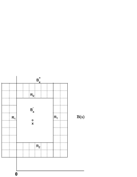
Figure 2: The placements of $B_{x}^{-},B_{x}^{+},R_{1}$ and $R_{2}$ are shown.

$B_{x}^{-}$ to be the rectangle of $(1+d_{x})\times 2$ centred at $x$ and $B_{x}^{+}$ to be the rectangle of $(\frac{7}{3}+d_{x})\times\frac{10}{3}$ centred at $x$. Divide the region of $B_{x}^{+}\backslash B_{x}^{-}$ into 64 small rectangles with two diffrent sizes: one size recorded $R_{1}$ is $\frac{1}{3}\times\frac{1}{3}$, and the other size recorded $R_{2}$ is $\frac{1+d_{x}}{6}\times\frac{1}{3}$, see Figure 2. The number of small rectangles with size $R_{1}$ is $40$, and the number of small rectangles with size $R_{2}$ is $24$. Define $A_{1}$ to be the event that each of these 64 small rectangles includes at least one point of $\mathcal{H}_{\lambda}$. By the properties of Poisson point processes, we have

$$\begin{aligned} P(A_{1})&=\left(1-e^{-\lambda/9}\right)^{40}\cdot\left(1-e^{-\lambda(1+d_{x})/18}\right)^{24}\\ &\geq\left(1-e^{-\lambda/9}\right)^{40}\cdot\left(1-e^{-\lambda/18}\right)^{24}.\end{aligned}$$ (39)

If $A_{1}$ happens, there exists a connected component in $B_{x}^{+}\backslash B_{x}^{-}$ which contains all the points in these small rectangles. Also, for any point in $\mathbb{R}^{d}\backslash B_{x}^{-}$ which can connect directly with a point in $B_{x}^{-}$, it must connect directly with this connected component. Let $A_{2}$ denote the event that there exists at least one point in $B_{x}^{+}\backslash B_{x}^{-}$ contained by $\mathcal{C}_{\infty}$. So according to above discussion, the event $A_{1}\cap A_{2}$ is independent with the distribution of the points of $\mathcal{H}_{\lambda}$ in $B_{x}^{-}$. Therefore,

$$P(A_{1}\cap A_{2})=P(A_{1})P(A_{2}|A_{1})\geq P(A_{1})p_{\infty}(\lambda).$$ (40)

Denote $A_{3}$ to be the event that there exists at least one point of $\mathcal{H}_{\lambda}$ in $B(x;1)\cap B(s)^{c}$, where $B(x;1)$ denotes the $d-dimensional$ unit ball centred at point $x$. By the properties of Poisson point processes it can be computed that

$$P(A_{3})=1-\exp\left(\lambda\left(d_{x}\sqrt{1-d_{x}^{2}}-\arccos d_{x}\right)\right).$$ (41)

Because $A_{3}$ and $A_{1}\cap A_{2}$ are both increasing events in $G(\mathcal{H}_{\lambda};1)$, by FKG inequality (Theorem 2.2 in [4]) we have

$$P(A_{3}\cap A_{1}\cap A_{2})\geq P(A_{3})P(A_{1}\cap A_{2}).$$ (42)

If the event $A_{3}\cap A_{1}\cap A_{2}$ happens, it must be true that $x\in\mathcal{C}_{\infty}$. Also, the event $A_{3}$ is independent with the distribution of the points of $\mathcal{H}_{\lambda}$ in $B_{x}^{-}$, so we have

$$\begin{aligned} P\left[\{|V_{x}|=1\}\cap\{x\in\mathcal{C}_{\infty}\}\right]&\geq P[A_{3}\cap A_{1}\cap A_{2}\cap\{\mathcal{H}_{\lambda}\cap B_{x}^{-}=\emptyset\}]\\ &=e^{-2(1+x)\lambda}P(A_{3}\cap A_{1}\cap A_{2})\\ &\geq e^{-4\lambda}P(A_{3}\cap A_{1}\cap A_{2}).\end{aligned}$$ (43)

Set $c:=e^{-4\lambda}\cdot\left(1-e^{-\lambda/9}\right)^{40}\cdot\left(1-e^{-\lambda/18}\right)^{24}$, together with (39), (40), (41), (42) and (43) we can get (38).

Let $W$ denote the number of the points of $\mathcal{H}_{\lambda}\cap B_{i}(\widetilde{x}_{s,a},a)$ which belong to $\mathcal{C}_{\infty}$ but are isolated in $B(s)$. By the definition of $\xi(B_{i}(\widetilde{x}_{s,a},a))$ and Palm theory for Poisson processes, we have

$$E[\xi(B_{i}(\widetilde{x}_{s,a},a))]\geq E[W]=\lambda\int_{B_{i}(\widetilde{x}_{s,a},a))}P\left[\{|V_{x}|=1\}\cap\{x\in\mathcal{C}_{\infty}\}\right]dx.$$

Combining this with (38), we can get $E[\xi(B_{i}(\widetilde{x}_{s,a},a))]>\frac{1}{2}c\left(1-e^{(1-\pi)\lambda/4}\right)\lambda p_{\infty}(\lambda).$ Our result follows.

Proof 2.6 (Proof of Theorem 1)

For simplicity of exposition, we shall prove (4) only in the case of $d=3$, and this proof has no essential difficulty in the case of $d=2$ or $d\geq 4$.

Let $\eta_{ij}(s):=E\left[\xi\left([0,1]\times[i,i+1]\times[j,j+1],s\right)\right]$ and take $n=\lfloor\frac{s}{2}\rfloor$. By symmetry we have $\eta_{ij}(s)=\eta_{ji}(s)$, and therefore

$$\begin{aligned} E\left[\xi\left([0,1]\times[0,n]^{2}\right)\right]&=\sum_{i=0}^{n-1}\sum_{j=0}^{n-1}\eta_{ij}(s)\\ &=\eta_{00}(s)+\sum_{k=1}^{n-1}\left(2\sum_{i=0}^{k-1}\eta_{ik}(s)+\eta_{kk}(s)\right).\end{aligned}$$ (44)

Set

$$a_{1}(s):=\eta_{00}(s)+\sum_{k=1}^{n-1}\left(2\sum_{i=0}^{k-1}\left(\eta_{ik}(s)-\eta_{i,n-1}(s)\right)+\eta_{kk}(s)-\eta_{k,n-1}(s)\right),$$

then for large $s$ and $s_{2}$ satisfying $s_{2}>s$, by Lemma 6 we have

$$\begin{aligned} &|a_{1}(s)-a_{1}(s_{2})|<2n^{2}e^{-cs/2}\\ &~{}~{}~{}~{}~{}~{}~{}~{}+\sum_{k=n}^{n_{2}-1}\left(2\sum_{i=0}^{k-1}|\eta_{ik}(s_{2})-\eta_{i,n_{2}-1}(s_{2})|+|\eta_{kk}(s_{2})-\eta_{k,n_{2}-1}(s_{2})|\right)\\ &<2n^{2}e^{-cs/2}+\sum_{k=n}^{n_{2}-1}\left(2\sum_{i=0}^{k-1}e^{-ck}+e^{-ck}\right)=o\left(e^{-cs/3}\right),\end{aligned}$$ (45)

where $n_{2}=\lfloor\frac{s_{2}}{2}\rfloor$ and $c$ is the same constant appearing in Lemma 6. Then by Cauchy’s criterion the limit of $a_{1}(s)$ exists.

Define the point $y_{i}=(0,i,n)\in\mathbb{R}^{3}$. For any $i\in[0,n-1]$ and large $s$, using Lemmas 6 and 7 we can get

$$\begin{aligned} &\big{|}E\left[\xi\left(B_{2}\left(y_{i},{\textstyle\frac{s}{2}}-n\right)\right)\right]-({\textstyle\frac{s}{2}}-n)\eta_{i,n-1}(s)\big{|}\\ &\leq\big{|}E\left[\xi\left(B_{2}\left(y_{i},{\textstyle\frac{s}{2}}-n\right)\right)\right]-({\textstyle\frac{s}{2}}-n)E\left[\xi\left([0,1]\times[i,i+1]\times[{\textstyle\frac{s}{2}}-1,{\textstyle\frac{s}{2}}]\right)\right]\big{|}\\ &~{}~{}~{}~{}~{}~{}~{}~{}+({\textstyle\frac{s}{2}}-n)\big{|}E\left[\xi\left([0,1]\times[i,i+1]\times[{\textstyle\frac{s}{2}}-1,{\textstyle\frac{s}{2}}]\right)\right]-\eta_{i,n-1}(s)\big{|}\\ &=o\left(e^{-cs/3}\right).\end{aligned}$$ (46)

Similarly, we can get

$$E\left[\xi\left([0,1]\times\left[n,\frac{s}{2}\right]^{2}\right)\right]=\left(\frac{s}{2}-n\right)^{2}\eta_{n-1,n-1}(s)+o\left(e^{-cs/3}\right).$$ (47)

We recall that $R_{0}=[0,1]\times[0,s/2]^{2}$, then together with (44), (45), (46) and (47),

$$\begin{aligned} E\left[\xi\left(R_{0}\right)\right]&=E\left[\xi\left([0,1]\times[0,n]^{2}\right)\right]+2\sum_{i=0}^{n-1}E\left[\xi\left(B_{2}\left(y_{i},\frac{s}{2}-n\right)\right)\right]\\ &~{}~{}~{}~{}~{}~{}~{}~{}~{}~{}~{}~{}+E\left[\xi\left([0,1]\times\left[n,\frac{s}{2}\right]^{2}\right)\right]\\ &=\sum_{k=1}^{n-1}\left(2\sum_{i=0}^{k-1}\eta_{i,n-1}(s)+\eta_{k,n-1}(s)\right)+\left(s-2n\right)\sum_{i=0}^{n-1}\eta_{i,n-1}(s)\\ &~{}~{}~{}~{}~{}~{}~{}~{}~{}~{}~{}~{}+\left(\frac{s}{2}-n\right)^{2}\eta_{n-1,n-1}(s)+a_{1}+o\left(e^{-cs/3}\right),\end{aligned}$$ (48)

where $a_{1}:=\lim_{s\rightarrow\infty}a_{1}(s)$. Let $b_{i}(s):=\eta_{i,n-1}(s)-\eta_{n-1,n-1}(s)$, then by (48) we have

$$\begin{aligned} E\left[\xi\left(R_{0}\right)\right]&=\left(\frac{s^{2}}{4}-1\right)\eta_{n-1,n-1}(s)+\sum_{k=1}^{n-1}\left(2\sum_{i=0}^{k-1}b_{i}(s)+b_{k}(s)\right)\\ &~{}~{}~{}~{}~{}~{}~{}~{}~{}~{}~{}~{}+\left(s-2n\right)\sum_{i=0}^{n-1}b_{i}(s)+a_{1}+o\left(e^{-cs/3}\right)\\ &=\left(\frac{s^{2}}{4}-1\right)\eta_{n-1,n-1}(s)+s\sum_{i=0}^{n-2}b_{i}(s)-2b_{0}(s)-\sum_{i=1}^{n-2}(2i+1)b_{i}(s)\\ &~{}~{}~{}~{}~{}~{}~{}~{}~{}~{}~{}~{}+a_{1}+o\left(e^{-cs/3}\right).\end{aligned}$$ (49)

Set

$$a_{2}(s):=\sum_{i=0}^{n-2}b_{i}(s)~{}~{}~{}\mbox{and}~{}~{}~{}a_{3}(s):=2b_{0}(s)+\sum_{i=1}^{n-2}(2i+1)b_{i}(s).$$

With the similar argument as (46), we can get that the exist constants $a_{2}$ and $a_{3}$ such that

$$|a_{2}(s)-a_{2}|<3ne^{-cs/2}~{}~{}~{}\mbox{and}~{}~{}~{}|a_{3}(s)-a_{3}|=o\left(e^{-cs/3}\right).$$

Also, by Lemmas 6 and the Cauchy’s criterion, there exists a constant $a_{0}>0$ such that

$$|\eta_{n-1,n-1}(s)-a_{0}|<e^{-c(n-1)}.$$

Taking $a_{0},a_{2}$ and $a_{3}$ into (49) we have

$$E\left[\xi\left(R_{0}\right)\right]=\left(\frac{s^{2}}{4}-1\right)a_{0}+sa_{2}-a_{3}+a_{1}+o\left(e^{-cs/3}\right).$$

with the similar argument as above, there exist constants $a_{4},a_{5},a_{6}$ and $a_{7}$, such that

$$E\left[\xi\left(R_{1}\right)\right]=\frac{s^{2}}{4}a_{0}+sa_{4}+a_{5}+o\left(e^{-cs/3}\right),$$

and

$$E\left[\xi\left(R_{2}\right)\right]=\frac{s^{2}}{4}a_{0}+sa_{6}+a_{7}+o\left(e^{-cs/3}\right).$$

Combined these with (10), (13) and Lemma 3, (4) has been deduced, where $\tau_{1}=6a_{0}>0$.

With the results of Theorem 10.22 and Theorem 11.16 (which shows that $\delta>0$) in [9], (4) is followed by (5).

Proof 2.7 (Proof of Theorem 2)

Given the discussion in the proof of Theorem 11.16 in [9], (2.45) in [9] is followed by

$$\left(n/\lambda\right)^{-1/2}\left(L_{1}\left(G\left(\mathcal{X}_{n};(n/\lambda)^{-1/d}\right)\right)-E[L_{1}(G(\mathcal{H}_{\lambda,s};1))]\right)\xrightarrow{D}\mathcal{N}(0,\delta^{2}),$$

where $s=(n/\lambda)^{1/d}$. Combining this and (4) our result follows.

3 Some Applications

Our method used in the proof of Theorem 1 can be applied to estimate the expectation of many other random variables restricted to a box $B$ as $B$ becomes large, for example, the size of the biggest open cluster for percolation, the coverage area of the largest component for Poisson Boolean model, the number of open clusters or connected components for percolation and Poisson Boolean model, the number of open clusters or connected components with order $k$ for percolation and Poisson Boolean model, the final size of a spatial epidemic mentioned in [9] and so on. We will give the similar results as Theorem 1 for the size of the biggest open cluster and the number of open clusters for site percolation but the method can be adapted to bond percolation.

Following Chapter 1 of [2], let $\mathbb{L}^{d}=(\mathbb{Z}^{d},\mathbb{E}^{d})$ denote the integer lattice with vertex set $\mathbb{Z}^{d}$ and edges $\mathbb{E}^{d}$ between all vertex pairs at an $l_{1}$-distance of 1. For $d\geq 2$ we take $X=(X_{x},x\in\mathbb{Z}^{d})$ to be a family of i.i.d. Bernoulli random variables with parameter $p\in(0,1)$. Sites $x\in\mathbb{Z}^{d}$ with $X_{x}=1(0)$ are denoted open (closed). The corresponding probability measure of on $\{0,1\}^{\mathbb{Z}^{d}}$ is denoted by $P_{p}$. The open clusters are denoted by the connected components of the subgraph of $\mathbb{L}^{d}$ induced by the set of open vertices. Let $C_{\textbf{0}}$ denote the open cluster containing the origin. The percolation probability is $\theta(p)=P_{p}(|C_{\textbf{0}}|=\infty)$ and the critical probability is $p_{c}=p_{c}(d):=\sup\{p:\theta(p)=0\}.$ It is well known [2] that $p_{c}\in(0,1)$. If $p>p_{c}$, by Theorem 8.1 in [2], with probability $1$ there exists exactly one infinite open cluster $\mathcal{C}_{\infty}$.

Given integer $n>0$, we denote by open clusters in $B(n)$ the connected components of the subgraph of the integer lattice $\mathbb{L}^{d}$ induced by the set of open vertices lying in $B(n)$. Similar results as Theorem 1 concerned with the order of the biggest open cluster in $B(n)$ can be given as follows.

Theorem 8

Suppose $d\geq 2$ and $p\in(p_{c},1)$. Let $H(X;B(n))$ be the order of the biggest open cluster in $B(n)$. Then there exist constants $c=c(d,p)>0$ and $\tau_{i}=\tau_{i}(d,p)$, $1\leq i\leq d$, with $\tau_{1}>0$, such that for all large enough $n$,

$$E_{p}[H(X;B(n-1))]=\theta(p)n^{d}-\sum_{i=1}^{d}\tau_{i}n^{d-i}+o\left(e^{-cn}\right).$$ (50)

Also, there exists a constant $\sigma=\sigma(d,p)>0$, such that

$$H(X;B(n-1))n^{-d/2}-\theta(p)n^{d/2}+\sum_{i=1}^{\lfloor\frac{d}{2}\rfloor}\tau_{i}n^{d/2-i}\xrightarrow{D}\mathcal{N}(0,\sigma^{2})$$ (51)

as $n\rightarrow\infty$.

Proof 3.1

Similar to the above, $E_{p}[|\mathcal{C}_{\infty}\cap B(n-1)|]=\theta(p)n^{d}$. Let $C_{1},C_{2},...,C_{M}$ denote the components of $\mathcal{C}_{\infty}\cap B(n-1)$, taken in a decreasing order. Let $L(n-1)=B(n-1)\backslash[1,n-2]^{d}$. For any $2\leq i\leq M$, since $C_{i}\subset\mathcal{C}_{\infty}$, therefore there exists at least one point in $L(n-1)\cap C_{i}$ which connects to $\mathcal{C}_{\infty}$ directly; we choose the smallest one according to the lexicographic ordering on $\mathbb{Z}^{d}$ as the $out-connect$ $point$. For any $x\in\mathbb{Z}^{d}\cap L(n-1)$, define

$$\xi(x):=\left\{\begin{array}[]{ll}|C_{i}|,&\mbox{if there exists }i\in[2,M]\mbox{ such that $x$ is the out-connect point of $C_{i}$},\\ 0,&\mbox{otherwise},\end{array}\right.$$

Also, for integer $j\in[0,d-1]$, let

$$R_{j}:=\left([0,1]\times[0,n-1]^{d-1-j}\times[1,n-2]^{j}\right)\cap\mathbb{Z}^{d},$$

then

$$E\left[\sum_{i=2}^{M}|C_{i}|\right]=\sum_{x\in\mathbb{Z}^{d}\cap L(n-1)}E[\xi(x)]=2\sum_{j=0}^{d-1}\sum_{x\in R_{j}}E[\xi(x)].$$

With the similar process as the proof of Theorem 1, (50) can be deduced, where

$$\tau_{1}=2d\lim_{n\rightarrow\infty}E\left[\xi\left(\left(0,\lfloor\frac{n}{2}\rfloor,\ldots,\lfloor\frac{n}{2}\rfloor\right)\right)\right]>0.$$

Using Theorem 3.2 in [8], (51) follows.

Following Chapter 1.5 of [2], we define the number of open clusters per vertex by

$$\kappa(p)=E_{p}(|C_{\textbf{0}}|^{-1})=\sum_{n=1}^{\infty}\frac{1}{n}P_{p}(|C_{\textbf{0}}|=n),$$

with the convention that $1/\infty=0$. Similar results as Theorem 1 concerning with the number of the open clusters in $B(n)$ can also be given as follows.

Theorem 9

Suppose $d\geq 2$ and $p\in(0,p_{c})\cup(p_{c},1)$. Let $H(X;B(n))$ be the number of the open clusters in $B(n)$. Then there exist constants $c=c(d,p)>0$ and $\tau_{i}=\tau_{i}(d,p)>0$, $1\leq i\leq d$, with $\tau_{1}>0$, such that for all large enough $n$,

$$E_{p}[H(X;B(n-1))]=\kappa(p)n^{d}+\sum_{i=1}^{d}\tau_{i}n^{d-i}+o\left(e^{-cn}\right).$$ (52)

Also, there exists a constant $\sigma=\sigma(d,p)>0$, such that

$$H(X;B(n-1))n^{-d/2}-\kappa(p)n^{d/2}-\sum_{i=1}^{\lfloor\frac{d}{2}\rfloor}\tau_{i}n^{d/2-i}\xrightarrow{D}\mathcal{N}(0,\sigma^{2})$$ (53)

as $n\rightarrow\infty$. Moreover, for any constant $\varepsilon\in(0,d/2)$,

$$\begin{aligned} &P_{p}\left(\frac{H(X;B(n-1))-\kappa(p)n^{d}-\sum_{i=1}^{d}\tau_{i}n^{d-i}}{\mbox{Var}(H(X;B(n-1)))}\leq x\right)\\ &=\int_{-\infty}^{x}\frac{1}{\sqrt{2\pi}}e^{-y^{2}/2}dy+o\left(n^{-\frac{d}{2}+\varepsilon}\right),\end{aligned}$$ (54)

where Var$(\cdot)$ denotes the variance.

Proof 3.2

Let $L(n-1)=B(n-1)\backslash[1,n-2]^{d}$. For any $x\in B(n-1)\cap\mathbb{Z}^{d}$, let $C_{x}$ denote the open cluster including $x$, and let $C_{x}(B(n-1))$ denote the open cluster including $x$ in $B(n-1)$. Then $C_{x}(B(n-1))\subseteq C_{x}$. For all open clusters $C$ in $B(n-1)$, if $C\cap L(n-1)\neq\emptyset,$ according to the lexicographic ordering on $\mathbb{Z}^{d}$ we choose the smallest element of $C\cap L(n-1)$ as the indicated vertex of $C$. For any $x\in\mathbb{Z}^{d}\cap L(n-1)$, define

$$\xi(x,B(n-1)):=\left\{\begin{array}[]{ll}1-\frac{|C_{x}(B(n-1))|}{|C_{x}|},&\mbox{if $x$ is the idicated vertex of $C_{x}(B(n-1))$},\\ 0,&\mbox{otherwise}.\end{array}\right.$$

Noted that for any $y\in\mathbb{Z}^{d}\cap B(n-1)$,

$$\sum_{x\in C_{y}(B(n-1))}\left(|C_{y}(B(n-1))|^{-1}-|C_{y}|^{-1}\right)=1-\frac{|C_{y}(B(n-1))|}{|C_{y}|},$$

then by (4.7) in [2], we have

$$\begin{aligned} H(X;B(n-1))&=\sum_{x\in\mathbb{Z}^{d}\cap B(n-1)}|C_{x}(B(n-1))|^{-1}\\ &=\sum_{x\in\mathbb{Z}^{d}\cap B(n-1)}|C_{x}|^{-1}+\sum_{x\in\mathbb{Z}^{d}\cap L(n-1)}\xi(x,B(n-1)).\end{aligned}$$ (55)

Therefore, take the expectation for the both sides of (55), we can get

$$E_{p}[H(X;B(n-1))]=\kappa(p)n^{d}+\sum_{x\in\mathbb{Z}^{d}\cap L(n-1)}E_{p}[\xi(x,B(n-1))].$$

Suppose $1\leq i\leq d$ and $x_{j}\in[0,K/2-1]\cap\mathbb{Z}$ for $1\leq j\leq i$. For large integers $n_{1},n_{2}$, let $x=(x_{1},\ldots,x_{i},\lfloor\frac{n_{1}}{2}\rfloor,\ldots,\lfloor\frac{n_{1}}{2}\rfloor)\in\mathbb{Z}^{d}$ and $\widetilde{x}=(x_{1},\ldots,x_{i},\lfloor\frac{n_{2}}{2}\rfloor,\ldots,\lfloor\frac{n_{2}}{2}\rfloor)\in\mathbb{Z}^{d}$. Set $\widetilde{B}(n_{2}):=B(n_{2})\oplus\{x-\widetilde{x}\}.$ Since $\xi$ is stationary under translations of the lattice $\mathbb{L}^{d}$, then $\xi(\widetilde{x},B(n_{2}))$ and $\xi(x,\widetilde{B}(n_{2}))$ have the same distribution function. However, let $n_{0}=\min\{\lfloor\frac{n_{1}}{2}\rfloor,\lfloor\frac{n_{2}}{2}\rfloor\}$, by the definition of $\xi$ we have

$$P_{p}\left[\xi(x,B(n_{1}))\neq\xi(x,\widetilde{B}(n_{2}))\right]=P_{p}\left[\xi(x,B(n_{1}))\neq\xi(x,\widetilde{B}(n_{2})),C_{x}\neq C_{\infty}\right]$$

$$~{}~{}\leq P_{p}\left[\mbox{diam}(C_{x})\geq n_{0},C_{x}\neq C_{\infty}\right]<e^{-cn_{0}},$$

where the last inequality follows from Theorem 6.1 of [2] for $p<p_{c}$ and Theorem 8.18 of [2] for $p>p_{c}$ respectively. Thus,

$$\left|E_{p}\left[\xi(x,B(n_{1}))\right]-E_{p}\left[\xi(\widetilde{x},B(n_{2}))\right]\right|$$

$$~{}~{}\leq\sum_{t}t\left|P_{p}\left[\xi(x,B(n_{1}))=t\right]-P_{p}\left[\xi(x,\widetilde{B}(n_{2}))=t\right]\right|$$

$$~{}~{}\leq\sum_{t}\left(P_{p}\left[\xi(x,B(n_{1}))=t,\xi(x,B(n_{1}))\neq\xi(x,\widetilde{B}(n_{2}))\right]\right.$$

$$~{}~{}~{}~{}~{}~{}~{}~{}~{}~{}\left.+P_{p}\left[\xi(x,\widetilde{B}(n_{2}))=t,\xi(x,B(n_{1}))\neq\xi(x,\widetilde{B}(n_{2}))\right]\right)$$

$$~{}~{}=2P_{p}\left[\xi(x,B(n_{1}))\neq\xi(x,\widetilde{B}(n_{2}))\right]<2e^{-cn_{0}}.$$

Therefore, $\lim_{n\rightarrow\infty}E_{p}[\xi(x,B(n)]$ exists. In fact, a similar result as Theorem 6 can be deduced. Let

$$\widetilde{\tau}_{i}(K)={{d}\choose{i}}\sum_{x_{j}\in[0,K-1]\cup[n-K,n-1],1\leq j\leq i}\lim_{n\rightarrow\infty}E_{p}\left[\xi\left(\left(x_{1},\ldots,x_{i},\left\lfloor\frac{n}{2}\right\rfloor,\ldots,\left\lfloor\frac{n}{2}\right\rfloor\right)\right)\right],$$

and let $\tau_{i}(K)=\sum_{j=1}^{i}\widetilde{\tau}_{j}(K){{d-j}\choose{i-j}}(-2K)^{i-j}.$ In a similar way, (52) is obtained.

Combining (52) with Theorem 3.1 in [8], (53) follows immediately.

By Theorem 2.1 in [5], Theorem 3.1 in [8] and (52), (54) can be deduced.

It is worth noting that our results do have significance for some practical applications. In fact, the initial motivation of this paper is to provide theoretical foundation and guidance for the design of wireless multihop networks. The wireless multihop networks, e.g., vehicular ad hoc networks, mobile ad hoc networks, and wireless sensor networks, typically consists of a group of decentralized and self-organized nodes that communicate with each other in a peer-to-peer manner over wireless channels, and are increasingly being used in military and civilian applications [12]. The large scale wireless multihop networks are usually formulated by the random geometric graphs, and the size of the largest component is a fundamental variable for a network, which plays a key role for the topology control in wireless multihop networks. However, this variable can not be described very precisely by both former theoretic results and even computer simulations as the scale of the network grows to very large. Theorem 1 and Theorem 2 provides a precise estimation for this variable respectively. Using simulations the approximative values of the parameters $p_{\infty}(\lambda)$, $\tau_{i}$, $\sigma$ and $\delta$ can be obtained, and thus the expression of the asymptotic size of the largest component can be well established, which has guiding significance to the topology control in wireless multihop networks.

This research was Supported by the National Natural Science Foundation of China under Grants No. 61203141 and 71271204, and the Innovation Program of the Chinese Academy of Sciences under Grant No. kjcx-yw-s7.

References

[1]Glauche, I., Krause, W., Sollacher, R. and Greiner, M.
(2003). Continuum percolation of wireless ad hoc communication
networks. Physica A: Statistical Mechanics and its
Applications325, 577–600.
[2]Grimmett, G. (1999). Percolation, 2nd edn. Springer,
Berlin.
[3]Hekmat, R. and Mieghem, P. Van. (2006). Connectivity in
Wireless Ad Hoc Networks with a Log-normal Radio Model. Mobile
Networks and Applications11, 351–360.
[4]Meester, R. and Roy, R. (1996). Continuum Percolation.
Cambridge University Press, New York.
[5]Jiang, J., Zhang, S. and Guo, T. (2010). A convergence rate in a martingale CLT for percolation clusters. Journal of the graduate school of the chinese academy of sciences27(5), 577-583.
[6]Penrose, M. (1991). On a continuum percolation model. Advances in Applied Probability30, 628–639.
[7]Penrose, M. (1995). Single linkage clustering and continuum
percolation. Journal of Multivariate Analysis53,
94–109.
[8]Penrose, M. (2001). A central limit theorem with applications
to percolation, epidemics and Boolean models. Annals of
Probability29, 1515-1546.
[9]Penrose, M. (2003). Random Geometric Graphs. Oxford
University Press, New York.
[10]Penrose, M. and Pisztora, A. (1996). Large deviations for
discrete and continuous percolation. Advances in Applied
Probability28, 29–52.
[11]Pishro-Nik, H., Chan, k., and Fekri, F. (2009).
Connectivity properties of large-scale sensor networks. Wireless
Networks15, 945–964.
[12]Ta, X., Mao, G., and Anderson, B.D.O. (2009).On the giant
component of wireless multihop networks in the presence of
shadowing. IEEE Transactions on Vehicular Technology58,
5152–5163.