A coronal wave as CME footprint

Abstract

Context. Coronal waves are disturbances propagating over a large portion of the solar disc. Despite the fact that they resemble a wave originating from a single point, several authors argue that they are due to the restructuring of the solar magnetic field during a coronal mass ejection.

Aims. I report a coronal wave observed in Fexii, soft X-ray, and H$\alpha$ on November 6, 2006, jointly with a CME and a flare to show the spatial and temporal relation of the wave and the CME. I also take advantage of the spectral resolution of the wave to obtain an approximation of its temperature. Finally, I compare the magnetic field topology to the wave location.

Methods. I overlay all the observations. To highlight the faint structures, and especially stationary structures produced on the passage of the wave, I use images obtained by subtracting a pre-event image from the observations then I apply wavelet transform. The temperature is obtained by comparing theoretical emissions to the ratio of the emission of the wave front through two different filters in soft X-ray. Using the synoptic magnetogram obtain with the Mickelson Doppler Imager (MDI/SoHO) and the Potential Field Source Surface (pfss) of the solar software (SSWIDL), I draw the magnetic field lines at the borders of the magnetic field topological domains.

Results. The observations show bright fronts that are co-spatial when observed at the same time, therefore I believe that the same wave is observed in the different band passes. The wave front is not observable in H$\alpha$, but just in Fexii and in soft X-ray, indicating that the temperature of the wave front is higher than the chromospheric temperature. The ratio of emission through two SXI filters gives a temperature of $7\ 10^{6}$ K for the wave front. The northern-most edge of the CME footprint related to this wave corresponds to the last location of the wave on the limb. The image processing reveals stationary brightenings produced on the passage of the wave front. The potential spherical extrapolation of the sun shows that those stationary brightenings are lying in jumps of magnetic field lines connectivity.

Conclusions. Coronal waves are hot structures. They are the footprint of a CME and are related to the magnetic field topology.

1 Introduction

Global coronal waves are large scale disturbances that can be observed in the solar atmosphere in coronal and chromospheric spectral wavelengths. H$\alpha$ waves were first discovered in association with flares and named Moreton waves (Moreton 1960, 1961, Moreton and Ramsey 1960). More recently, waves were observed in Fexii, usually named EIT waves (Dere et al. 1997, Thompson et al. 1998, Attrill et al. 2007, Long et al. 2008), and finally in soft X-rays (Khan and Hudson 2000, Khan and Aurass 2002; Narukage et al. 2002). These waves are bright structures that usually propagate in a restricted arc, narrow in H$\alpha$, thicker and diffuse in Fexii, traveling on the solar disc across distances that can be up to the solar radius. Their morphology and evolution may be compared to surface gravity waves propagating on the surface of a water.

Warmuth et al. (2004) show that when the waves appear in H$\alpha$, EUV and soft X-ray spectral band passes simultaneously, they are nearly co-spatial. The study conducted in Warmuth et al. (2004) is in contradiction with other observational studies: e.g. Eto et al. (2002) who found the Moreton wave to precede the diffuse coronal wave, and Klassen et al. (2000). The later reference analyzes in detail several coronal waves observed in Fexii, compares their velocities to the usual values given in the literature and concludes that the coronal waves are slower than the Moreton waves. However, Vršnak et al. (2002) indicate several properties of the dynamic (deceleration of the coronal wave front) and the observation of the Fexii waves (low cadence of images and visibility of the EIT waves much farther than the Moreton waves) that have to be taken into account to resolve this discrepancy. For example, Eto et al. (2002) find that the wave fronts observed in H$\alpha$ and in Fexii have different velocities and conclude that the coronal wave is physically distinct from the H$\alpha$ wave. However, going through the data set again, one can find that the flare related to the emission of the wave begins 4 min. earlier than the first image obtained by EIT (Extreme ultra-violet Imaging Telescope, Delaboudinère et al. 1995) showing the flare and peaked 1 min. later. In H$\alpha$, the wave front is clearly visible over 12 min., beginning 1 min. after the EIT image showing the flare, ending just before the second EIT image of the event showing the flare, i.e. the first one showing the EIT wave. Due to the low cadence of images of EIT, this set of data cannot give a clear spatial correspondence between the EUV and H$\alpha$ wave. Regarding the velocities of each wave fronts derived from the observations, as the edge of the wave fronts are very different (in EUV it is diffuse, and sharper in H$\alpha$), differences in estimation of location of the border of each waves can give different estimation of the velocities, that may have lead Eto et al. (2002) to find different velocities for the two wave fronts. Co-spatial H$\alpha$ and Fexii wave fronts are studied using observations in Fexii and in H$\alpha$ obtained at the same time (e.g. Warmuth et al. 2004; Delannée et al. 2007; Thompson et al. 2000). Each of these studies conclude that the observed H$\alpha$ and Fexii wave fronts are co-spatial. Therefore, I believe that the Moreton wave and the EIT wave are the two manifestations of the same structure and I disregard any interpretation of the H$\alpha$ and Fexii being two structures moving at different speed (e.g. Eto et al. 2002; Chen et al. 2002).

Balasubramaniam et al. (2007) show that, when a Moreton wave passes through a filament, it can be enhanced in both the H$\alpha$ line center and in the wings of the line. This fact contradicts the amplitude of the wave estimated from the thickness of the front and the Doppler shift of the plasma inside the front. Therefore, Balasubramaniam et al. (2007) suggest that the Moreton waves are possibly high coronal structures emitting in H$\alpha$. Gilbert et al. (2004) show for two events that the observations of wave fronts in Hei and in Fexii data are co-spatial. If the chromospheric emission would have been due to a magnetosonic wave propagating in the chromosphere then due to the much denser medium the speed of this wave would have been much slower and the overlay of the two emissions (chromospheric and coronal) would not have been possible. Therefore, Gilbert et al. (2004) conclude that the chromospheric emission of the wave front is not due to a wave propagating in the chromosphere but is rather an imprint of a disturbance in the corona. I also believe that the chromospheric emission of the observed waves is due to a high altitude structure that can sometime produce emission in lower temperature. Wills-Davey et al. (2007) noted that the coronal waves are frequently observed only in Fexii without any H$\alpha$ nor soft X-ray counterpart. Therefore, what kind of physical process can make the wave sometime observable and other time invisible in H$\alpha$? This question also rises from this study.

Biesecker et al. (2002) compare the occurrence of a coronal wave in the catalog established by Thompson and Myer (2009) with the occurrence of a flare that is defined by a significant, impulsive, transient increase in X-ray flux recorded by NOAA GOES 3 X-ray monitor. Looking at well defined and less defined coronal waves (see the catalog given in Thompson and Myer 2009, for an explanation of the confidence level of the occurrence of a wave), Biesecker et al. (2002) find that only 66 of the 173 observed waves, occurred in conjunction with a flare that is defined by a significant, impulsive, transient increase in X-ray flux recorded by NOAA GOES 3 X-ray monitor. This relation seems very low as I do not know any detailed study of a coronal wave that appears without any flare. In that sens, Cliver et al. (2005) show that very week (A-class) flares can be related to Fexii waves, indicating that the definition of a significant increase in X-ray flux may impact the results obtained by Biesecker et al. (2002). Cliver et al. (2005) note that Moreton waves were closely associated with flares during 1960-1970 - indeed they were often referred to as flare waves . Taking the idea of coronal waves and Moreton waves as the same structure, they both appear to be produced together with a flare from which they both seem to originate. Therefore, many studies modeled them as magnetosonic waves propagating freely in the solar corona, originating from a pressure pulse that also produces the flare (Warmuth et al. 2007 and references therein).

Coronal waves can appear conjointly with type II radio emission (Klassen et al., 2000). As the type II are radio emission slowly decreasing in frequency, they are commonly interpreted as signature of waves steepening into shocks and propagating outwards through the corona (Wild and McCready, 1950; Nelson and Melrose, 1985). The association of the type II radio burst and the coronal wave reinforces their interpretation in terms of magnetosonic waves. However, Wills-Davey et al. (2007) discussed several reasons why the observed coronal waves cannot be magnetosonic waves. The principal counterargument is that the observed structures have a large range of velocities (from 100 to 400 km s^-1), meaning that the coronal conditions have to be quite different at different time which seems unreasonable. Another counterargument is that the magnetosonic waves have to find quite high plasma beta values to persist over large distances: in Wu et al. (2001) for example, a ring shaped wave propagates on the solar surface, but the simulation is performed using $\beta>1$ everywhere in the corona, which is much higher than the typical value used in other articles (i.e. $\beta=0.01$) to study coronal phenomenon. I would like to add to these counterarguments that the corona is very structured. Due to interaction between photospheric magnetic flux concentrations, the coronal plasma $\beta$ may vary a lot from very low value (less than 1) close to the flux concentration, to high values (more than 1) where the interaction of the flux concentration almost annuls the coronal magnetic field (Gary et al. 2001, Warmuth et al. 2005). These variations may exist even in a small area. In these conditions, a magnetosonic wave mode would be very deformed, reflected, dissipated, or converted to another mode when it encounters a magnetic structure, i.e. active regions, filaments and bright points, which are everywhere on the solar disc, hindering the propagation of a self-similar structure over large distances. I note here that, in the numerical simulations performed in Wang et al. (2000), even if the plasma $\beta$ is quite high and the conversion into another wave mode is not taken into account, the structure of the initial atmosphere (in density and in magnetic field) deforms the simulated wave making it different to the observed one during the final stages of simulation. Finally, Podladchikova & Berghmans (2007) show that the ring shaped observed coronal waves present patches of high light intensity. Podladchikova & Berghmans (2007) and Attrill et al. (2007), show that these patches are rotating. The rotation of the ring shaped observed coronal waves cannot be modeled by a freely propagating magnetosonic wave. Therefore, I disregard any freely magnetosonic wave model for the observed wave structures.

Even though it may be stated that every wave appears in conjunction with a flare, most flares do not produce any observable coronal waves (Delannée and Aulanier 1999, Cliver et al. 2005, Chen et al. 2006), so the flares do not seem to be the origin of the waves but a counter part of another phenomenon as well as the wave itself. The statistical analysis performed in Biesecker et al. (2002), shows that there is a strong correlation between the Fexii wave and the CMEs. Even if this study is biased by errors or threshold while doing the catalogs, this result is confirmed by studies on smaller numbers of individually observed events. Warmuth et al. (2004, 12 events) and Delannée et al. (2000, 17 events) both find that 100% of Fexii waves are produced in conjunction with a CME. I also note that I do not know a published case of a Fexii wave produced without any CME. So, I believe that each coronal wave is related to a CME where it finds its origin. These two facts, i.e. the lack of a coronal wave for every flare and the presence of a CME in conjunction with a coronal wave, lead several authors to interpret coronal waves in terms of signatures of CMEs that are due to magnetic field lines opening: piston driven waves/shocks (Thompson et al. 2000; Chen et al. 2002; Cliver et al. 2005; Warmuth et al. 2005), electric currents and plasma compression generated by expanding magnetic field lines (Delannée and Aulanier 1999, Delannée et al. 2008), magnetic field line reconnection in the quiet Sun induced by the CME expansion (Attrill et al. 2007). These interpretations imply that every coronal wave is the footprint on the solar disc of a CME.

Vršnak et al. (2006) and Patsourakos & Vourlidas (2009) compare the locations of the CME leg and of the wave front, both of them find that the wave moves ahead of the CME leg, contradicting the models given in the previous paragraph. On the other hand, Chen (2009), Attrill et al. (2009) and Cohen et al. (2009) provides examples of events on the limb showing a strong spatial mapping between the CME and the coronal wave. In this article, I study a coronal wave that appeared on November 6, 2006 on the east limb associated with a CME to determine whether the coronal wave is the CME footpoint or not. I analyze this event using Derotated Base Difference Image (DBDI) processing (Delannée & Aulanier 1999, Thompson et al. 2000) instead of the usual running difference images used in Vršnak et al. (2006) and Patsourakos et al. (2009). This last process reveals the brightness variation of structures from one image to the following one: if a structure is bright in an image and remains as bright in the following one, it appears gray in the running difference images; if the brightness of the structure is still high but a bit decreased, the structure appears dark in the running difference image. In the case of the coronal waves, they are commonly described as a bright front surrounding a dimmed region (see e.g. Thompson et al. 1998, Warmuth et al. 2004). This description comes from the use of the running difference images, but appears to be (partly) an artifact of this process because the brightness of the wave front slowly decreases with the time (Delannée et al. 2007). If instead of using the previous image to be subtracted with its following one, I use an image obtained before the appearance of the structure, then the same structure with slowly decreasing brightness would appear bright on two consecutive images obtained after the subtraction. So doing DBDI allows to reveal structures that last for a long time even if its brightness decreases. The correction of the solar rotation is very needed as the sun may rotate quite a lot in the time interval of the two images used to obtain a DBDI. Using the DBDI method, Delannée et al. (2007) showed that a coronal wave appears to have a slightly different morphology and behavior than using the running difference images.

Delannée & Aulanier (1999), Delannée (2000) Delannée et al. (2007), Attril et al. (2007a,b) Attrill et al. (2009) and Cohen et al. (2009) study 8 coronal waves using DBDI processing of data. They find that the coronal waves are not fully propagating: some portion of the wave reach a final location that remain bright for 10 min. to one hour depending on the spectral band pass used for the observations. Delannée and Aulanier (1999), Delannée et al. (2007) and Delannée (2009), Attrill et al. (2009) and Cohen et al. (2009) reveal that the stationary brightenings of the coronal waves are lying in jumps of connectivity of magnetic field lines. These jumps of connectivity are known to be sites at which electric current is easily produced (Sweet 1958; Aulanier et al. 2006). The existence of electric currents are related to occurrence of hot coronal structures (Magara and Longcope 2001). Therefore Delannée and Aulanier (1999) and Delannée et al. (2007) conjecture that the stationary brightenings of the coronal waves are due to Joule heating in the jumps of magnetic field line connectivity. Doing the image processing of instrument observations and comparing the occurrence of structures with extrapolated magnetic field topology is a very long study to lead therefore, until today, only five coronal waves are studied using this processing. On this basis, Warmuth et al. (2004) claim that the stationary brightenings are very rare and that this electric current model cannot be suited to explain the occurrence of the large majority of coronal waves. I am using this same processing of analysis to find several properties of a coronal wave: its link with the CME (is it lying at the footprint of the CME leg?), its dynamics (is it propagating or stationary?) and its temperature (is it a cool or hot structure?). Sec. 1 presents the data used in this study. Sec. 2 analyzes the data and Sec. 3 summarizes the analysis and concludes on the relation between the CME and the wave.

2 Data

2.1 Instruments of observations

I investigate simultaneous multi-wavelength data. The soft X-ray images are obtained with the Soft X-ray Imager (SXI, Pizzo et al. 2005) on board the Geosynchronous Operational Environmental Satellite 13 (GOES-13). The image cadence is about one minute. Four different filters are used: Polyimide Thin , Polyimide Thick , Beryllium Thin , Tin ; therefore the cadence of images is about 4 minutes for each filter. All these filters are sensitive to light emission from hot plasma with temperatures ranging from 1 to 10 MK. The extreme ultra-violet images at 195 Å are obtained using the Extreme ultra-violet Imaging Telescope (EIT, Delaboudinière et al. 1995) on board the Solar and Heliospheric Observatory (SoHO). The cadence of these images is 12 minutes. This filter is mainly sensitive to the emission of Fexii present at about 1.5 MK. The H$\alpha$ images are obtained using the Optical Solar Patrol Network (OSPAN) at the Sacramento Peak Observatory. The cadence of images is about one minute. The H$\alpha$ line ($\lambda=6365\AA$) is sensitive to plasma at a temperature of $10^{4}$ K. The images of the upper corona are obtained using the orange filter of Large Angle Solar Coronagraph C2 (LASCO, Brueckner et al. 1995) on board SoHO. This filter is mainly sensitive to the plasma density as its band pass is very broad.

2.2 Extrapolated magnetic field

The magnetogram and the spherical potential magnetic field extrapolations come from the potential field source surface package from Solarsoft in the Interactive Data Language (pfss/SSWIDL, Schrivjer and deRosa 2003). A synoptic magnetogram is constructed from the data obtained with the Michelson Doppler Imager (MDI/SoHO, Scherrer et al. 1995), and updated every 4 hours to include the data near the central meridian of the sun. The synoptic magnetogram on November 6, 2006 does not show any strong magnetic polarity in the area of the eruption. This is likely because there was not any magnetic polarity during the previous solar rotation and because the flare is behind the limb. After November 7, 2006 the magnetogram shows a magnetic bipole appearing from behind the limb in the south, at the longitude of the flare site. This bipole is close to the central meridian on November 13, where it is well resolved. Unfortunately, between November 7 and 13, it evolves expanding, rotating, emerging, dispersing. This evolution might influence the magnetic field topology during this period. The PFSS runs at the Lockheed Martin Solar and Astrophysics Laboratory (LMSAL) using a synoptic magnetogram to extrapolate the potential magnetic field over the whole solar surface. The results are just retrieved on a local computer where a small procedure of visualization permits to draw a selection of magnetic field lines. Drawing the magnetic field lines that have one footpoint close to each other and the other one the farthest from each other, I locate the limits of the domains of connectivity of the magnetic field lines. I checked the magnetic field topology evolution of the region affected by the wave from November 7 to 13: it remains quite similar despite the distortion of the magnetic bipole.

Moreover, McIntosh et al. (2007) explain the refilling of coronal loops that are opened during an eruption by the reformation of the pre-eruptive topology. Similarly, Lynch et al. (2008) show that after an eruption the magnetic field reconfigures to its pre-eruption topology in a numerical simulation of an eruption. These considerations allow me to use a synoptic magnetogram obtained at a later time than the day of the eruption to compare its topology to the structures appearing during the wave front propagation.

As commonly observed, the large scale magnetic field is potential (e.g. Delannée and Aulanier 1999; Wang et al. 2002), even in active regions, the magnetic field shear is much less than 1 Mm^-1 (Mandrini et al. 2002). Therefore, potential magnetic field is suitable for comparison to the structures appearing during the event of November 6, 2006, as it affects a large portion of the Sun.

I choose to use the data obtained on November 10, 2006 at 12:04 UT, the closest in time from the eruption in which the dipole seems resolved enough. The potential magnetic field lines extrapolated from the synoptic magnetogram obtained on November 10, 2006, are shifted to correct the rotation of the Sun between November 6 and 10, in order to allow an overlay with the observations of November 6.

2.3 DBDIs

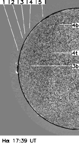
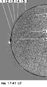
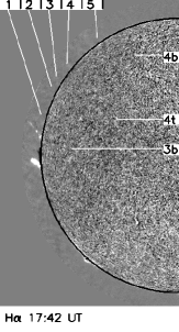
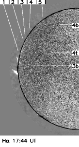
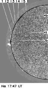
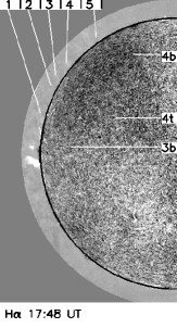
Figure 2: DBDIs obtained by the OSPAN instrument using a large band pass filter centered on the H$\alpha$ spectral emission line. The numbers indicate the successive appearance of the wave in SXI. The field of view contains half of the solar disc and is overlaid to the field of view of images in Figs. 3 and 6. A small prominence is erupting from behind the limb at 17:40 UT. One small brightness is visible at the position 1 from 17:44 UT to 17:47 UT. Except for this brightening, no Moreton wave is visible neither on the limb nor on the disc.

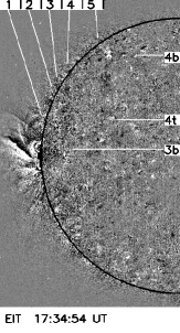
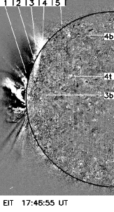
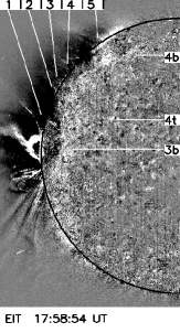
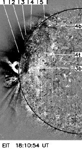
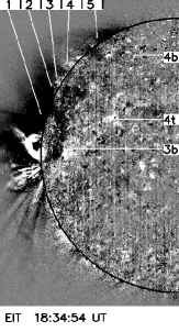
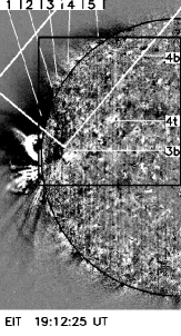
Figure 3: DBDIs obtained using the 195 Å filter of EIT. Half of the solar surface is shown. The numbers indicate the successive appearance of the wave in SXI. The field of view contains half of the solar disc and is overlaid to the field of view of images in Figs. 2 and 6. The large white rectangle on the last panel shows partly the sub-field of view of the images displayed in Fig. 4. The large black rectangle on the last panel shows the sub-field of view of the images displayed in Fig. 5. The EIT wave is observed progressing from an active region located slightly behind the limb to the northern coronal hole where it stops. The last position of the EIT wave above the limb is very darkened after 18:10 UT. On the disc, the EIT wave progresses from the active region to the east, and stops at bright point pointed by labels.

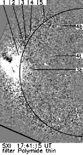
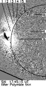
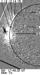
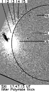
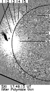
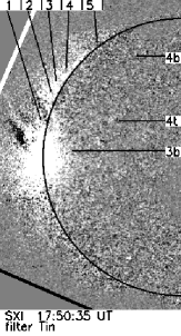
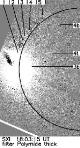
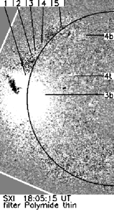
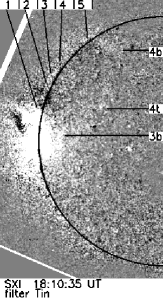
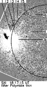
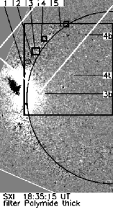
Figure 6: DBDIs obtained using SXI. The names of the filters used are written on each image. Remark that the brightness of the structures is slightly different in the different images. The numbers indicate the successive appearance of the wave. The field of view contains half of the solar disc and is overlaid to the field of view of images in Figs. 2 and 3. The small squares on the last panel show the area over which the mean brightness is measured and presented in Fig. 13. The large white rectangle on the last panel shows the sub-field of view of the images displayed in Fig. 7. The large black rectangle on the last panel shows the sub-field of view of the images displayed in Figs. 8 and 9. The SXI wave is observed progressing from an active region located slightly behind the limb to the northern coronal hole and to an eastern location where it stops. All the positions taken by the wave, comprising its latest position, stay very bright until 18:26 UT in most of the SXI filter.

The H$\alpha$, Fexii and soft X-ray images are Derotated Base Difference Images (DBDIs): each image is corrected for the differential rotation to the time of the first SXI image at 17:25 UT before being subtracted with an image obtained using the same filter at the closest time before the beginning of the flare (i.e. 17:39 UT). The wave appears partly above the limb and partly on the solar disc. I used an old version of the drot_map from the solarsoft to correct the solar differential rotation. This old version add, without any correction, the over-limb observation to the corrected on disc one. Therefore, the over-limb observed structures presented in the figures of this article are not affected by any correction. In an image corrected for the solar rotation for a short period of time, the structures on the disc and close to the limb are corrected by only a very small shift (2 EIT pixels, 1.4 SXI pixel and 0.13 pixels of Figs. 2, 3 and 6 at the equator and close to the limb during the 2 hours duration of the event) ensuring continuity between the structures on the disc and the ones above the limb. The DBDIs presented here are highly contrasted to show the very small brightness changes of the structures, which makes the DBDIs quite noisy.

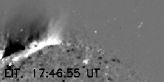
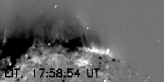
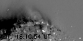
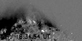
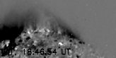
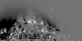
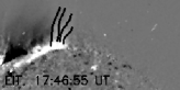
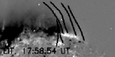
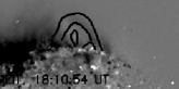
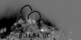
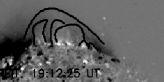
Figure 4: Sub-field of view, shown in the white rectangle in the last panel of the Fig. 3, focusing on the over-limb structures observed in 195 Å. The images are highly processed (see the text). The second line shows the same images as in the first line but with some over-limb structures highlighted with black drawings.

I try to highlight the structures as much as possible by highly processing them. I apply several filters during the processing, which results in the DBDIs presented in Figs. 3 and 6. The images in Figs. 4 to 9 (with the exception of those in Fig. 6) are obtained by summing 4 neighboring pixels then expanding the images to their original size. This first process smooths the intensity spatial variation, removing the isolated flickering pixel. Then, the intensity of each pixel is replaced by the hyperbolic tangent of its intensity, which permit to exaggerate the faint structure while minimizing the flickering pixels. The images presented in Fig. 4 undergo this process solely.

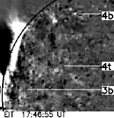
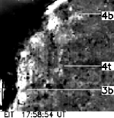
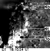
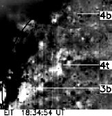
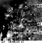
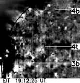
Figure 5: Sub-field of view, shown in the black rectangle in the last panel of the Fig. 3, focusing on the on-disc structures appearing during the wave front passage observed in 195 Å.

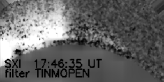
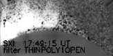
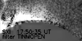
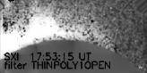
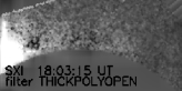
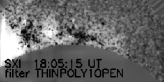
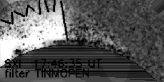
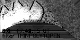
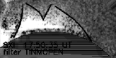
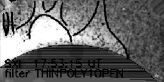
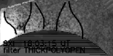
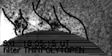
Figure 7: Same sub-field of view as in Fig. 4, focusing on the over-limb structures observed in SXI. The images are highly processed (see the text). The second line show the same images as in the first line but with some over-limb structures highlighted with black drawing. The name of the filters are THINPOLYOPEN for Polyimide thin, THICKPOLYOPEN for Polyimide thick, TINMOPEN for Tin.

The images in Figs. 5, 7 undergo a wavelet filtering removing the spatial frequencies less than 20 pixels. This wavelet transform permits to obtain an image showing the large scale variations at the typical scale of the wave front observed in Fexii. However, the wave front is formed of both small and large structures. So, the wavelet transformed image is used as a third filter to be multiplied by the original DBDI.

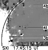
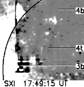
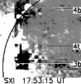
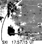
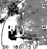
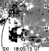
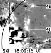
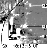
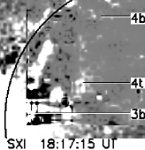
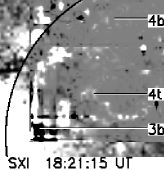
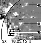
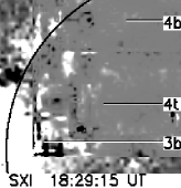
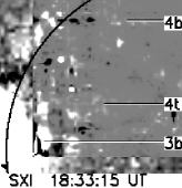
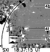
Figure 8: Same on disc sub-field of view as in Fig. 5, focusing on the stationary brightenings labeled 3b, 4b and 4t, through the ”Polyimide Thin” filter. The images are highly processed to highlight the brightenings (see the text).

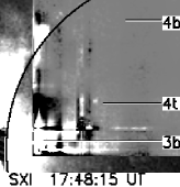
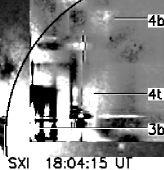
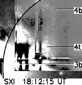
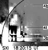
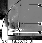
Figure 9: Same on disc sub-field of view as in Fig. 5, focusing on the stationary brightenings labeled 3b, 4b and 4t, through the ”Polyimide Thick” filter. The images are highly processed to highlight the brightenings (see the text).

The soft X-ray observations are very contaminated by the scattered light of the flare. Therefore I choose a sub-field of view to cut as much as possible the flaring site, while retaining as much as possible of the wave front motion. The first wavelet transform of SXI data is chosen to remove any signal smaller than 12 pixels and larger than 70 pixels, permitting to remove a part of the scattered light due to the flare. The intensity spatial variation is then fitted to a 5 degree polynomial surface using the sfit function of IDL. The smoothed surface is removed from the filtered image to obtain an image without the scattered light emission. Finally, this image is multiplied by the original DBDI to obtain the images presented in Figs. 8 and 9.

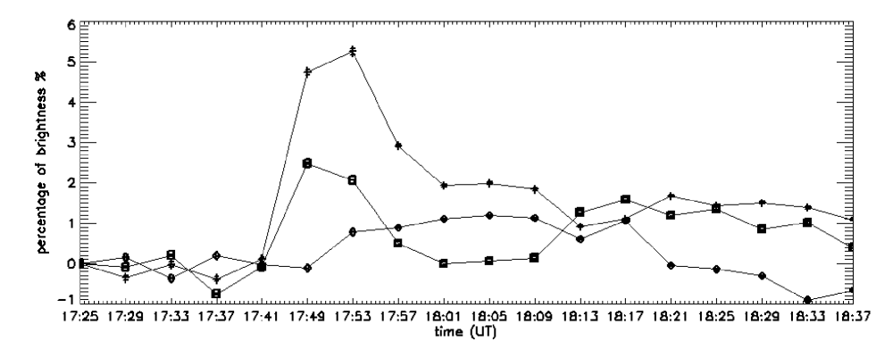
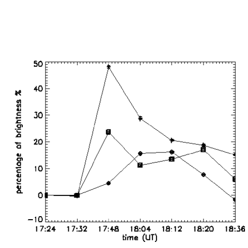
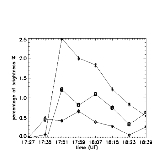
Figure 13: Curves of the percentage increase of the mean intensity in the squares drawn in the image at 18:36 UT in Fig. 6 with the initial mean intensity in the same areas plot against the time, using the ”Polyimide Thin” filter (top panel), the ”Polyimide Thick” filter (low left), and the ”Beryllium ThinA” filter (low right). Crosses are for the area 2, squares for 4 and diamonds for 5. Superimposed points give the error made on their values. The light curves reveal the propagation of the wave front above the limb, each reached location remaining bright for a while.

All of this processing creates artifacts. The summing of pixel removes the flickering pixels but smooths the signal to the neighboring pixels, increasing the spatial expansion of the signal of the wave. The wavelet transform removes the flickering pixels and the bright points, however some bright points are clearly observed with increasing intensity during the passage of the wave front, and maybe slightly before the passage of the wave front. Therefore, applying this process removes a part of the wave front signal. Moreover, the parameters used for the wavelet transform enhance the interference fringes, due to the grill supporting the filters, which could not be removed by the cleaning functions of SSWIDL. The fringes appear as horizontal and vertical straight lines that overlay and perturb the signal of the wave front. Finally, the 5^th degree polynomial surface fitting the spatial variation of the intensity in SXI, oscillates close to the border of the field of view, and does not fit the signal very well. After the subtraction of the fitted polynomial surface as a background, the image shows some artificial increase or decrease of the brightness close to the border of the sub-field of view. The highly processed images are not used to obtain the plots in Fig. 13. All the structures described in the following section are verified in the raw observations, to be sure that they are not artifacts of the processing. For comparison between the DBDI and the processed images, I present them both. All the images in Figs. 2, 3 and 6 are co-aligned and have the same field of view, showing the western half solar disc. The images with a field of view above the limb (see Figs. 4 and 7) are also co-aligned and are rotated so that extended structures in altitude appear to be vertical. In the same way, the on-disc subfield-of-view image (see Figs. 5, 8 and 9) are all co-aligned and show the same field of view.

Several movies of the observations are provided on line to make their description clearer to the reader. All the images used in the movies are DBDIs, have the same field of view and are separated by spectral emission lines.

The LASCO images are difference images obtained by subtracting a pre-event image. They are overlaid with the closest in time EIT DBDI.

3 Analysis

3.1 Phenomenology

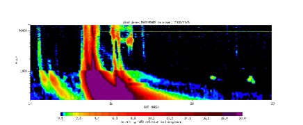
Figure 1: Type II radio emission obtained at Sagamore Hill Observatory. The radio emission begins at 17:39 UT.

On November 6, 2006, the wave is observed together with a C8.8 flare and a CME traveling through the LASCO/C2 field of view at a speed of 976 km s^-1 (according to CACTUS/SIDC software). The flare strength determined by the soft X-ray emission intensity is likely a minimum as the source region (likely AR 0923) is located slightly behind the east limb in the southern hemisphere (S06). The GOES 13 satellite detects the beginning of the flare at 17:43 UT, but radio emission is detected by the Sagamore Hill Observatory as early as 17:39 UT (Fig. 1). The H$\alpha$ images show that a small prominence is ejected into the corona at the location of the flare visible in SXI and in EIT (see Fig. 2 and the H$\alpha$ movie). The source region of the eruption may be a magnetic bipole located in AR 0923. Correcting the solar rotation from November 10th 12:04 UT to November 6th 17:17 UT, I estimate that the active region is located approximately 15^∘ behind the eastern limb at the time of the eruption. Of course, this method of estimation of the location of the active region behind the limb cannot take into account the migration, the emergence and the distortion of the active region that can shift its location in the 4 days delay between the observation and the date by which the active region is visible on the solar disc.

The wave is clearly visible in two band passes: in Fe xii and in soft X-ray; in H$\alpha$, it is possibly observed at only one location. When it is observed at approximately the same time in EIT and SXI the wave front is almost co-spatial (see detailed description of the observations here after, and Fig. 8). Therefore, I believe that this set of data presents multi-wavelength observations of the same structure. The wave moves from the southern hemisphere across the equator to the northern hemisphere and extends onto the disc toward the central meridian. The wave seems to originate from the flare site even if its propagation is not isotropic around this location. Between the flare and the wave front, a dimmed region develops (e.g. Figs. 3, 6).

I now compare the three sets of observations in each band pass in detail. The H$\alpha$ data does not show very much of the wave. A very small brightening appears at 17:44 UT at location 1 on Fig. 2. It has faded out at 17:47 UT. No motion of this brightness is visible. Therefore, it could be a stationary brightening of the Moreton wave. However, the differencing processing reveals the earth atmospheric turbulence effect on the image that appears as flickering bright and dark patches at the limb. So, the brightening appearing at location 2 in H$\alpha$ could also be a seeing artifact revealed by the difference of images technique. I checked in the images obtained in the red and blue wings of the H$\alpha$ spectral line if any signal of a Moreton wave could appear, and did not find any.

In EUV, the EIT wave front defines the border of a dimming (Fig. 3 and the EIT movie). This front is large, wide and diffuse. It propagates from the flare site to the northern pole and on the disc from the eastern limb to the central meridian (see the bright arch in panels of Fig. 5). On the disc, it stops at locations reached at 18:10 UT staying brighter than before the eruption for about one hour (see especially the bright diffuse arch linking the brigth points labeled 3b, 4b and 4t on the disc in Figs. 3 and 5). Above the limb, the wave front is formed of elongated in altitude structures (Fig. 4, image at 17:46 UT). The last observed position of the front is obtained at 17:58 UT at label 5 (Figs. 3 and 4). From 18:10 UT to at least 19:34 UT, the location 5 is dimmer than prior to the flare. Between the locations 2 and 5 (Figs. 3 and 4) and after 18:10 UT, a very faint brightness illuminates coronal loops above the limb, that are dimmed in the image at 17:58 UT. This brightness morphology does not resemble to the wave front that passed on its way from the south to the north: its wideness (in the range of 250-300 Mm at the limb at 18:34 UT and 18:46 UT) is too large (the wave front wideness is 87 Mm and 131 Mm at 17:46 UT and 17:58 UT resp.) and it does not move between 18:34 UT and 19:12 UT. It could be very hardly the reflection of the wave front on the northern coronal hole. Between the wave and the flare sites a large dimmed area develops.

The bright front observed in SXI is also made of structures elongated in altitude (see the almost radial structures above the limb in Figs. 6 and 7). Every location reached by the SXI wave on the limb stays very bright until 18:26 UT. Therefore, the wave front is wider in SXI ($\approx 246$ Mm) than in EIT ($\approx 87$ Mm) at early time (see the elongated structures above the limb at 17:46 UT in 195 Å  in Fig. 4 and in soft X-ray in Fig. 7). Later, the wideness of the wave front becomes of the same order in the two band passes ($\approx 158$ Mm in SXI and $\approx 131$ Mm in EIT, at 17:58 UT at the location 5). As every locations reached by the wave front remain bright for few minutes at the early stage, a dimmed region between the flare and the wave front, takes few minutes to develop: it appears after 17:57 UT between locations 5 and 4 and extends to reach location 2 at 18:05 UT. This dimming is overlaid to the one observed in EIT, but it is less deep and uniform than in EIT.

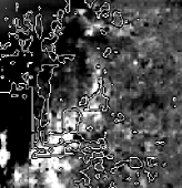
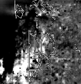
Figure 10: Right (left) image is an overlay of the Fexii at 18:10 UT and contours of the emission through the ”Polyimide Thin” at 18:13 UT (”Polyimide Thick” at 18:12 UT, resp.).

The SXI wave front on the disc is not clearly visible as it is more diffuse and appears in a more noisy environment due to the presence of many bright points. At 17:45 UT the wave front passes on the disc. The bright point at location 3b is illuminated since 17:45 UT (see Fig. 6) and is fully co-spatial to the one observed in Fexii at 17:46 UT. The same location appears dark in Figs. 8 and 9, because the polynomial fitted surface of the scattered light that is removed as a background from the images, oscillates close to the border of the selected sub-field of view. This oscillation is not real and the dark appearance of the location 3b is an artifact of the processing of image. The wave front appears as a faint arch that can be overlaid to the Fexii wave front, having the same shape and behavior (Fig. 10). It illuminates some bright points on it passage, for example 4t appears at 17:49 UT and 4b at 18:05 UT, both last until 18:37 UT in the Polyimide Thin data. 4b is almost disappeared at 18:20 UT in the Polyimide Thick data.

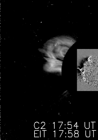
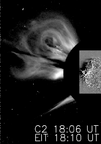
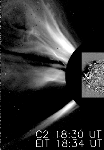
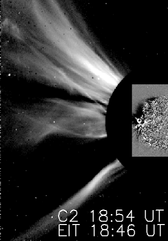
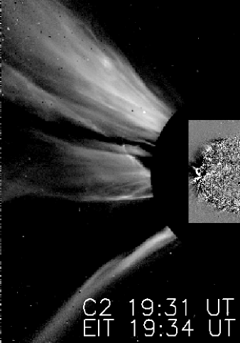
Figure 11: Overlay of the same DBDIs obtained with the EIT data and BDIs obtained with LASCO C2. The dimming sector close to the solar disc can be extended to the sector covered by the brightness in LASCO C2. The northern leg of the CME in the first image at 17:58 UT corresponds to the brightness appearing where the EIT and SXI wave stops in its farther north and last location.

The LASCO C2 images show the CME related to this event (Fig. 11). The CME appears in the northern east quadrant of the corona at 17:54 UT. On the combined LASCO/EIT images, the sides of the CME can be drawn back to the limb and intersects the most in the north location of the EIT wave front at 17:58 UT (location 5 in Fig. 6). In EUV, this location then dims. After 18:10 UT some loops are brightened (see label 4 in Fig. 6). Again the CME leg can be drawn back to the solar limb and intersects those brightened loops. The southern CME leg is related to the southern edge of the flare. I note that a jet located in the southern hemisphere appears during the CME. This jet is progressing at the same speed than the CME. Its shape seems deformed and enlightened by the progression of the CME.

3.2 Some understanding in light of magnetic field topology

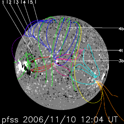
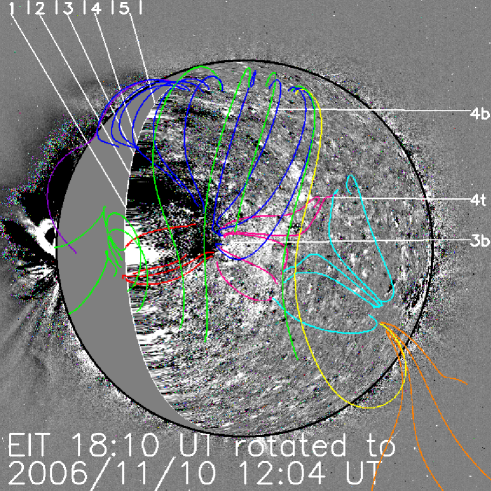
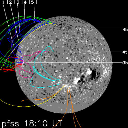
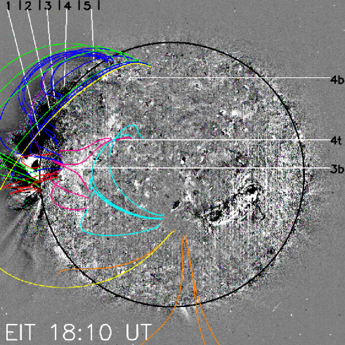
Figure 12: Magnetic map (left) and BDBI at 195 Å  (right) overlaid with some magnetic field lines that define some magnetic jumps of connectivity rotated to November, 10 2006 at 12:04 UT (upper) and to November, 6 2006 at 17:25 UT (lower). The stationary brightenings are lying in magnetic field lines jumps of connectivity.

The pfss extrapolation of the region involved in the event gives some understanding of those structures (Fig. 12). The magnetic field lines are drawn in different colors to highlight the magnetic field topology. Despite the fact that the projection on November 6 (lower left panel of Fig. 12), makes the green magnetic field lines appearing closed, connecting the northern pole to the active region, the projection on November 10 (see upper panel of Fig. 12) show that they are not connected at all. Those green lines are all opened (i.e. they connect the solar surface to the source surface of the high corona), they have the same orientation, entering inside the sun. The orange ones are also opened but in the inverse orientation, connecting the source surface to the positive magnetic polarity of AR 0922 located S09 W13. The red ones connect the location 3b to the flaring region. The blue ones connect the location 3b to the northern coronal hole. The pink ones connect the location 3b to the location 4t. The cyan ones connect the southern coronal hole in AR 0922 to the location 4t.

A coronal hole lies between the eastern limb and AR 0923 (see the open green magnetic field lines on the left upper panel of Fig. 12). I checked the stability of this coronal hole. The extrapolation of the magnetic field shows this coronal hole from November 5 to November 13 2006, even if the magnetic polarity in AR 0923 changes during those 8 days. As frequently observed the waves are not crossing coronal holes (Thompson et al. 1999). So, I believe that the eruption takes place close to red magnetic field lines drawn in the southern hemisphere on the magnetic map of November, 10 2006. The EUV dimming located between the flare site and the locations 1 and 3b is under these red lines indicating that some of those magnetic field lines are expanding during the eruption.

The stationary brightenings 3b, 4b and 4t are lying in drastic jumps of magnetic field lines connectivity: 3b is at the footpoints of the red and pink magnetic field lines, 4t at the footpoints of the pink and cyan ones, 4b at the footpoints of the blue and green ones. A fainter brightness, visible in EIT on the disc in the southern east quadrant, lies in the pink magnetic field lines (see the lower right panel of Fig. 12). This brightness does not cross the pink magnetic field lines footpoints which are close to the cyan ones. The pink magnetic field lines define the limit of a topological domain. The blue magnetic field lines also show the approximate location of the limit of a magnetic topological domain. If the red magnetic field lines are opening, they produce the perturbation of these limits (blue, pink magnetic field lines and at location 3b, 4b and 4t) in which the plasma can be heated, and brightened in soft X-rays. The blue and pink magnetic field lines are possibly not opened during the eruption. When the blue magnetic field lines are viewed as on November 6, 2006, they are all superposed onto the plane of the sky, therefore, during the eruption they will be observed as bright elongated structures or loops that are very close to each other, as it is in fact observed in SXI. The stationary brightenings visible on the limb in SXI at label 5, and on the disc between the label 5 and 4b are lying at the edge of the northern coronal hole, at the footpoints of the blue and green magnetic field lines. Again, during the eruption, this limit of magnetic field domain is perturbed producing the heating of the plasma that is observed as bright points.

The orange magnetic field lines projected onto the plane of the sky on November, 6 2006 has the shape of the perturbed streamer observed on the LASCO C2 images (lower left panel of Fig. 12). Therefore, the distortion of those orange magnetic field lines is possibly due to the expansion of the red ones that push them. As those magnetic field lines also define the limit of a magnetic field line connectivity, the plasma is heated, producing its brightening.

I here note that the described phenomenon resembles to the one in Terradas and Ofman (2004). In this article, the top of the loops present over density and are compared to the brightened loops that enter in oscillation while an observed wave passes through them. This phenomenon cannot be applied to explain the observed structures in the present study as none loops present a brightened apex, on the contrary, or they are brightened all along their length or only their footpoints are brightened. The reason is that to produce the kind of oscillation presented in Terradas and Ofman (2004), the motion of the perturbation has to be transverse to the loop direction, and in our observations, the pfss extrapolation reveals that the motion of the perturbation is along the magnetic field lines.

3.3 Temperature

I now estimate the temperature of the wave front, focusing on the elongated structures that have their footpoint at locations 2, 4 and 5. As the coronal wave is almost not visible in H$\alpha$, it is made of hot plasma. The most in the north location of the wave front, labeled 5, and the location 4 (Fig. 6), emits light that passes through the ”Polyimide Thick” filter from 18:04 UT to 18:12 UT. In the same interval of time, the same locations are very dimmed in EUV (see image at 18:10 UT in Fig. 3). The temperature range of the emission in SXR is from 1 to 10 MK and in EUV the temperature of the principal spectral emission line Fexii is about 1.5 MK. Therefore, the SXR brightness located at the labels 5 and 4, is due to plasma with temperature higher than $1.5\ 10^{6}$ K. I estimate the mean emission over areas located above the limb near the labels 2, 4 and 5 from 17:24 UT to 18:36 UT (see the squares on the image at 18:36 UT in Fig. 6). The percentage increase of the mean light intensity over the initial mean light intensity in each filter and in each area is plotted against the time in Fig. 13. The signal of the wave in the ”Beryllium Thin A” filter is not detectable which is confirmed by the DBDI images (see the movie) - the increase of emission through this filter is due to the scattered light of the flare, proved by the fact that the emission decreases from position 2 to position 5 at the same time and also monotonic decreases with the time at each location - therefore the coronal wave temperature is less than 10 MK.

Through the ”Polyimide Thin” and ”Polyimide Thick” filters the temporal intensity variations show an abrupt increase at 17:49 UT (17:48 UT) at location 4 and at 17:53 UT (18:04 UT, resp.) at location 5, revealing the propagation of the wave front and also that the position 5 is weakly affected by the scattered light of the flare. All light curves verify that each location remains bright for several minutes. At the location 5, the brightness continues to increase for a while, then decreases slowly. At location 4, the intensity through the ”Polyimide Thin”’ filter is less than prior to the eruption between 17:57 UT and 18:09 UT, corresponding to the formation of the dimmed region, but then increases and stays quite high until the end of the sequence of observations.

The intensity variations are very small, of order of $0.5-2.5\%$ more than prior to the eruption through the ”Beryllium Thin A” filter, of $1-5.5\%$ through the ”Polyimide Thin” filter and of $10-30\%$ through the ”Polyimide Thick” filter. The errors made on these estimates are due to a statistical enlightening of a pixel hit by a photon that does not come from the pointed structures. The standard deviation $\sigma$ of a sample of N pixels with $x_{i}$ brightness is:

$$\sigma=\sqrt{\frac{1}{N}\sum^{N}_{i=1}{(x_{i}-\overline{x})}}$$ (1)

The statistical error is at most 2 % through the ”Beryllium Thin A” and ”Polyimide Thin” filter, and 20 % through the ”Polyimide Thick” filter. These errors are quite small due to rather large surface of integration of the brightness, which enlarge the sample of pixels and, therefore, reduces the statistical error. Another source of error is the difficulty to locate the border of the illuminating structure. Therefore the same quantities are computed over the same area enlarged at border by 3 pixels along the equator direction, then reduced by 3 pixels along the equator direction. The quantities are shown to fluctuate by at most 1 % through the ”Beryllium ThinA” and ”Polyimide Thin” filters, and 16 % through the ”Polyimide Thick” filter. This fluctuation is reduced if the area of integration is enlarged, and increased if the area of integration is reduced. This confirms that the border of the chosen area to integrate the brightness is very close to the border of the studied structures and explains the small error made. The propagated error of the variation of average brightness, $\overline{x}(t)$, against the time, t, is given by:

$$\Delta\left(\frac{\overline{x}(t)-\overline{x}(0)}{\overline{x}(0)}\right)=\frac{\Delta\overline{x}(t)}{\overline{x}(0)}+\frac{\overline{x}(t)^{2}}{\overline{x}(0)^{4}}\Delta\overline{x}(0)$$ (2)

where

$$\Delta\overline{x}(t)=\sigma(t)+\left|\overline{x}(t)-\max(\overline{x}_{-3}(t),\overline{x}_{+3}(t))\right|$$ (3)

$\sigma(t)$ is given by equation 1 at each time of observation, and $\overline{x}_{-3}(t)\ (\overline{x}_{+3}(t))$ is the average brightness over the reduced (enlarge, respectively) area at each time of observation. The propagated error is also small (at most 2 % through the 3 filters) due to the presence of the ratio between 2 quantities presenting similar errors. Therefore the temporal variations of the increase of the average brightness presented is Figure 13 can be trusted. However, these variations at location 2 are affected by the light emitted by the flare and scattered in the instrument. This error is very difficult to estimate as the pixels at the flare site are saturated, leading to the impossibility (up to now) to find a good fit of this scattered light.

Then I divide the mean emissions passing through the filters ”Polyimide Thick” over the mean emission passing through the filter ”Polyimide Thin”. The ratios appear to be very constant over the time, except at 18:37 UT, and over the locations: $\approx 0.477$. Using the plots of the ratio of responses from various filters given in Lemen et al. (2004) as a function of temperature, I find that the observed ratio corresponds to a temperature $\approx 7\ 10^{6}$ K for every brightenings. I note that the brightness of the location 2 is quite affected by scattered light, leading to a very poor confidence in the results at this location but this scattered light is very low at the location 5 leading to a more accurate estimate of the temperature.

The brightenings in SXI decrease after 18:26 UT to become even darker than prior to the eruption. As these new appearing dimmings are also visible at the same time in EUV, I suggest that the plasma is very depleted in this region, and that, as the plasma is depleted deeper with the time, the brightness due to the increase of temperature created on the passage of the wave can no longer persist. The depletion may have balanced the temperature increase producing the dimming in a wide range of temperature in the same region.

4 Discussion

The wave is barely visible or even invisible in H$\alpha$ which can be due to the fact that the temperature of the wave is higher than the chromospheric temperature. As it has been shown in other studies, the H$\alpha$, Fexii and SXR wave fronts are co-spatial when observe during a same event. I fully believe that the lack of emission of the studied wave front is due to a particular physical parameter of this wave. The plasma could be too hot but also it is possible that the morphology of the wave front influences its observability. The Fexii and the SXI emissions are very faint above the limb because the structures are seen from their sides leading to a low accumulation of their emission in their optically thin plasma. For the same reason of geometry, above the limb, the H$\alpha$ emission could be too faint to be detected. However, the part of the wave front propagating on the disc is also not visible, which could be due to the total absence of the H$\alpha$ emission in this studied wave.

As many other cases of coronal wave observed conjointly in H$\alpha$ and in coronal emissions are presented in the literature, I ask the question: what additional process may lead to the observability of these waves in H$\alpha$ that is missing in the present case. Several authors believing that the observed coronal waves are magnetosonic waves suggest that the H$\alpha$ wave are different magnetosonic wave mode than the coronal wave mode, therefore, in the present case, this magnetosonic wave mode should be not generated. Others suggest that the coronal wave can sometime dig into the corona to produce the H$\alpha$ emission, therefore, in the present case, the wave should be too weak to dig in the chromosphere. However, I remind to the reader that several arguments discredit the magnetosonic wave model for the observed wave, leading me to disregard this model and the interpretation that the H$\alpha$ emission is not a different wave than the coronal one. I know other coronal structures that can emit in H$\alpha$ (prominences, post-flare loops), I here suggest that the additional process could be a thermal cooling instability that appears only in some particular plasma conditions of temperature and density. This suggestion is already proposed by Delannée et al. (2008) and Balasubramaniam et al. (2007). It supports also the observations obtained by Delannée et al. (2007). In this latter study, the H$\alpha$ wave front is slightly shifted inside the Fexii wave front, which could indicate that the wave front emits at coronal wavelength and takes some few time to emit in H$\alpha$, as it would be in a case of thermal cooling instability.

The coronal wave front is found to be footprint of the CME leg. This is in contradiction with Vršnak et al. (2006) and Patsourakos and Vourlidas (2009), who both conclude that the coronal wave front is ahead of the CME leg. However, the DBDI method is not used in the latter analysis which instead use running difference images. This method is not suited to detect slowly inflating brightenings like the ones found in our set of observations. Doing running difference images of a fading bright slowly inflating structure produces a dark feature enclosed by a bright and sharp border. Therefore, the brightenings produced by a coronal wave cannot be well represented using the running difference image process and can produce the discrepancy between the wave front location and the CME leg as the one shown in the Fig. 4c in Vršnak et al. (2006) and in the Figure 4d in Patsourakos and Vourlidas (2009).

5 Conclusion

I present conjoint observations in H$\alpha$, in soft X-ray and in 195 Å of a coronal wave. The bright front observed in the two last wavelengths are co-spatial when observed together, so it seems very unlikely that they are different structures. The wave does not emit in H$\alpha$.

The observability of the coronal wave in soft X-ray indicates that it is a hot coronal structure with temperature $\approx 7$ MK. This means that heating processes are at work to form the coronal wave. This conclusion is coherent with the one given by Wills-Davey et al. (2000) from the observation of a coronal wave in Fexii that is not well observable in Feix (the temperature of formation of this spectral line is about 1.3 MK).

The wave is not exactly fully propagating when analyzed using DBDI: it produces stationary brightenings (bright points and elongated in altitude structures) on its passage then stops (the diffuse arch stops). All these produced structures last for tens of minutes in soft-X ray and about one hour in 195 Å. The existence of stationary brightenings of the so-called coronal waves is also coherent with 6 previous observations (Delannée and Aulanier 1999, Delannée 2000, Delannée et al. 2007a, Attrill et al. 2007a). This event is the first one obtained close to the limb, and in soft X-ray, presenting stationary brightenings.

This is the fourth case studied using DBDI and comparison with magnetic field topology (see also Delannée and Aulanier 1999 and Delannée et al. 2007, Delannée 2009). For these four studies the stationary brightenings produced on the solar disc on the passage of the coronal wave are lying in jumps of connectivity of the magnetic field lines.

The wave is produced conjointly with a CME. This is coherent with the conclusion of Biesecker et al. (2002): a wave is always accompany by a CME. This observation also shows that the final last produced stationary brightening is the footprint on the sun of one leg of the CME appearing above the coronagraph occulter. The dimmings close to the solar limb are located inside the CME footprint.

The wave front consists of elongated in altitude structures that draw the lower parts of magnetic field lines perturbed or opening during the CME.

A streamer is also observed disturbed, taking a small curve as if there was a wave propagating along it. The brightness of the streamer increases as well as its thickness. This perturbation appears during the evolution of the CME, just 12 minutes after the first appearance of the CME. The magnetic field extrapolation shows that the streamer is rooted at the border of a coronal hole where the wave also stops. All these facts show that the coronal wave, the CME and the perturbation of the streamer are connected through perturbation of the large scale magnetic field lines.

There exist several models of those three phenomenons. The models of the coronal waves can be divided in two types: magnetosonic wave or signature of the magnetic field restructuring during the opening of magnetic field lines. Studying only one event cannot permit to distinguish between those two origins. However, I exclude the first possible mechanism for the reasons given in the introduction section. I believe that the coronal waves are the edges of the same opening magnetic flux tube that also produce the observed CME (Delannée et al. 2007, 2008). This last model is supported by the observations and the analysis performed in this article.

The type II burst observed during this coronal wave could be interpreted as the presence of a shock. This fact led Khan and Aurass (2002) to reject the idea that coronal waves are a signature of opening of the magnetic field lines, and to reassure that the coronal waves are magnetosonic shocks. However, it seems to me that the presence of the type II conjointly with a coronal wave has to be more studied from the point of view of the opening magnetic field line model.

- (1) Aulanier, G., Pariat, E., Démoulin, P. & DeVore, C.R. 2006, Sol. Phys., 238, 347
- (2) Attrill, G., Harra, L., van Driel-Gesztelyi, L., Démoulin, P. 2007, ApJ, 656L, 101
- (3) Balasubramaniam, K. S., Pevtsov, A. A., Neidig, D. F. 2007, ApJ, 658, 1372
- (4) Biesecker, D. A., Myers, D. C., Thompson, B. J., Hammer, D. M., Vourlidas, A. 2002, ApJ, 569, 1009
- (5) Brueckner, G. E., Howard, R. A., Koomen, M. J., Korendyke, C. M. 1995, Sol. Phys., 162, 357
- (6) Chen, P. F., Wu, S. T., Shibata, K., Fang, C. 2002, ApJ, 572, L99
- (7) Chen, P. F., Fang, C., Shibata, K. 2005, ApJ, 622, 1202
- (8) Chen, P. F. 2006, ApJ, 641L, 153
- (9) Cliver, E. W., Laurenza, M., Stolini, M., Thompson, B. J. 2005, ApJ, 631, 604
- (10) Delaboudinière, J.-P., Artzner, G. E., Brunaud, J. et al. 1995, Sol. Phys., 162, 291
- (11) Delannée, C. and Aulanier, G. 1999, Sol. Phys., 190, 107
- (12) Delannée, C., Hochedez, J. F., Aulanier, G. 2007, A&A, 465, 603
- (13) Delannée C. 2009, A&A, 495, 571
- (14) Delannée, C., Török, T., Aulanier, G., Hochedez, J.-F. 2008, Sol. Phys., 247, 123
- (15) Dere, K. P., Brueckner, G. E., Howard, R. A. et al. 1997, Sol. Phys., 175, 601
- (16) Eto, S., Isobe, H., Narukage, N. et al. 2002, PASJ, 54, 481
- (17) Gary, G. A. 2001, Sol. Phys., 203, 71
- (18) Gilbert, H. R., Holze, T. E., Thompson, B. J., Burkepile, J. T. 2004, ApJ, 607, 540
- (19) Khan, J. I., Hudson, H. S. 2000, GRL, 27, 1083
- (20) Khan, J. I., Aurass, H. 2002, A&A, 383, 1018
- (21) Klassen, A., Aurass, H., Mann, G., Thompson, B. J. 2000, A&AS, 141, 357
- (22) Klimchuk, J. A. 2001, Proc. of the Chapman Conference on Space Weather, AGU, Geophysical Monograph Series 125, (eds) Song, P., Singer, H., Siscoe, G., 143
- (23) Lemen, J. R., Duncan, W., Edwards, C. G., Friedlaender F. M., Jurcevich, B. K., et al. 2004, ”The solar x-ray imager for GOES”, Proc. SPIE 5171, Telescopes and Instrumentation for Solar Astrophysics, 65
- (24) Long D. M., Gallagher, R. T., Mc Ateer, R. T. J., Bloomfield, D. S. 2008, ApJ, 680, 81
- (25) Lynch, B. J., Antiochos, S. K., DeVore, C. R., Luhmann, J. G., Zurbuchen, T. H. 2008, ApJ, 683, 1192
- (26) Magara, T., Longcope, D. 2001, ApJ, 559, 55
- (27) Mandrini, C. H., D moulin, P., Schmieder, B., Deng, Y. Y., Rudawy, P. 2002, A&A, 391, 317
- (28) McIntosh, S. W., Leamon, R. J., Davey, A. R., Wills-Davey, M. J. 2007, ApJ, 660, 1653
- (29) Moreton, G. E. 1960, AJ, 65, 494
- (30) Moreton, G. E., Ramsey, H. E. 1960 PASP, 72, 357
- (31) Moreton, G. E. 1961, S.&T., 69, 145
- (32) Narukage, N., Hudson, H. S., Morimoto, T., Akiyama, S., Litai, R., Kurokawa, H., Shibata, K. 2002, ApJ, 572, L109
- (33) Patsourakos, S. and Vourlidas, A. 2009, ApJ, 700, L182
- (34) Pizzo, V. J., Hils, S. M., Balch, C. C. et al. 2005, Sol. Phys., 226, 283
- (35) Scherrer, P. H., Bogart, R. S., Bush, R. I., Hoeksema, J. T., Kosovichev, A. G. 1955, Sol. Phys., 162, 129
- (36) Schrivjer, C., deRosa, M. 2003, Sol. Phys., 212, 165
- (37) Terradas, J., Ofman, L. 2004, ApJ, 610, 523
- (38) Thompson, B. J., Plunket, S. P., Gurman, J. B. et al. 1998, Geophys. Res. Letters, 25, 2461
- (39) Thompson, B. J., Gurman, J. B., Neupert, W. M. et al. 1999, ApJ, 517, L151
- (40) Thompson, B. J., Reynolds, B., Aurass, H. et al. 2000, Sol. Phys., 193, 161
- (41) Uchida, Y. 1968, Sol. Phys., 4, 30
- (42) Vrsnak, B., Warmuth, A., Temmer, M., et al. 2006, A&A, 448, 739
- (43) Wang, Y.-M. 2000, ApJ, 543, L89
- (44) Wang, T., Yan, Y., Wang, J., Kurokawa, H., Shibata, K. 2002, ApJ, 572, 598
- (45) Warmuth, A., Vrsnak, B., Aurass, H., Hansmeier, A. 2001, ApJ, 560L, 105
- (46) Warmuth, A., Vrsnak, B., Magdalenić, J., Hanslmeier, A., Otruba, W. 2004, A&A, 418, 1101
- (47) Warmuth , A., Mann, G., Aurass, H. 2005, ApJ, 626L, 121
- (48) Warmuth, A. 2007, The high Energy Solar Corona Waves, Eruptions, Particules, Lecture Notes in Physics, 725, 107
- (49) Wills-Davey, M. J., Thompson, B. J. 1999, Sol. Phys., 190, 467
- (50) Wills-Davey, M. J., DeForest, C. E., Stenflo, J. O. 2007, ApJ, 664, 556
- (51) Wu, S. T., Zheng, H., Wang, S., et al. 2001, J. Geophys. Res., 106, A11, 25089
- (52) Wu, S. T., Li, B., Wang, S., Huinan Zheng 2005, J. Geophys. Res., 110, A11, 102,
- (53) Zarro, D. M., Sterling, A. C., Thompson, B. J., Hudson, H. S., Nitta, N. 1999, ApJ, 520, L139