Scalable Visibility Color Map Construction in Spatial Databases

Abstract

Recent advances in 3D modeling provide us with real 3D datasets to answer queries, such as “What is the best position for a new billboard?” and “Which hotel room has the best view?” in the presence of obstacles. These applications require measuring and differentiating the visibility of an object (target) from different viewpoints in a dataspace, e.g., a billboard may be seen from two viewpoints but is readable only from the viewpoint closer to the target. In this paper, we formulate the above problem of quantifying the visibility of (from) a target object from (of) the surrounding area with a visibility color map (VCM). A VCM is essentially defined as a surface color map of the space, where each viewpoint of the space is assigned a color value that denotes the visibility measure of the target from that viewpoint. Measuring the visibility of a target even from a single viewpoint is an expensive operation, as we need to consider factors such as distance, angle, and obstacles between the viewpoint and the target. Hence, a straightforward approach to construct the VCM that requires visibility computation for every viewpoint of the surrounding space of the target, is prohibitively expensive in terms of both I/Os and computation, especially for a real dataset comprising of thousands of obstacles. We propose an efficient approach to compute the VCM based on a key property of the human vision that eliminates the necessity of computing the visibility for a large number of viewpoints of the space. To further reduce the computational overhead, we propose two approximations; namely, minimum bounding rectangle and tangential approaches with guaranteed error bounds. Our extensive experiments demonstrate the effectiveness and efficiency of our solutions to construct the VCM for real 2D and 3D datasets.

I Introduction

Recent advances in large-scale 3D modeling have enabled capturing urban environments into 3D models. These 3D models give photo-realistic resembling of urban objects such as buildings, trees, terrains etc. and are widely used by popular 3D mapping services, e.g., Google Maps, Google Earth, and Bing Maps. The increasing availability of these realistic 3D datasets provides us an opportunity to answer many real-life queries involving visibility in the presence of 3D obstacles. For example, a tourist may check the visibility of a new year firework event from different locations in the surrounding areas so that he can pick a good spot to enjoy it; an apartment buyer may want to check visibility of near-by sea-beach and mountains from various available apartments; and an advertising company may wish to determine visibility of their existing billboards from surrounding areas and find a suitable location for a new billboard accordingly.

In this paper, we investigate efficient techniques to answer the underlying query required by the above applications: computing visibility of an object (e.g., firework event, billboard) from the surrounding continuous space, or that of the surrounding space from a source viewpoint. Our target applications treat visibility as a continuous notion—e.g., a billboard may be more visible from one location than another, depending on factors such as distance, viewing angle, and obstacles between the viewpoint and the target. We therefore use a visibility function that provides real-valued visibility measures of various points in the (discretized) 3D space, where the visibility measure of a point denotes its visibility from the viewpoint or to the target object. Thus, the answer to our target query is essentially the visibility measures for every point in the 3D space. The result can be graphically represented as a heat map, by assigning colors to various points according to their visibility measures. We call this a visibility color map (VCM) of the space for a given target or for a given viewpoint.

Recent works have shown how database techniques can enable efficiently answering various types of visibility queries in the presence of obstacles. Various nearest neighbor (NN) queries consider visibility of objects [1, 2, 3]; for example, the visible nearest neighbor query [1] finds the nearest neighbors that are visible from the source. However, these works, like various other computer graphics works [4, 5, 6, 7, 8, 9], treat visibility as a binary notion: a point is either visible or not from another point. In contrast, in our target applications, visibility is a continuous notion. Recently, Masud et al. proposed techniques for computing continuous visibility measure of a target object from a particular point in 3D space (e.g., computing visibility of a billboard from a given location) [10]. On the contrary, our target applications require visibility calculation from or of a continuous space where there is no specific viewpoint.

One straightforward way to generate a VCM is to descretize the 3D space and to use the techniques in [10] to compute visibility measure for each discrete point in the space. However, this can be prohibitively expensive. For example, discretizing the surrounding space into 1000 points in each dimension would give a total of $10^{9}$ points in the 3D space; and computing visibility measure for each point by using techniques in [10] would take 128 days! The huge cost comes from two sources: (i) computing the visibility measure based on the distance and angle from all viewpoints, which is computationally expensive and (ii) accessing a large set of obstacles from the database, which is I/O expensive.

We address the above challenges with a three-step solution that uses several novel optimizations to reduce computational and I/O overhead. First, we partition the dataspace into a set of equi-visible cells, i.e., all points inside a cell have equal visibility of the target object in terms of visual appearance. We exploit the key observation that when a lens (e.g., a human eye) sees an object without any obstacles, it cannot differentiate between its visual appearances from a spatially close set of points within an angular resolution (or spatial resolution) of $\approx 4$ arcminutes ($\approx 0.07$ degrees) [11]. Thus, we can safely prune the visibility computation for a large number of viewpoints within the angular or spatial resolution without affecting viewer’s perception. This optimization significantly reduces the computation cost, as we can compute only one visibility measure for each cell.

In the next step, we consider the effect of obstacles. We compute visible regions, the regions in the space from where the target object is completely visible in the presence of obstacles. In the final step, we assign visibility measures to these regions from the corresponding cells by spatial joins. Both steps are I/O and computation intensive. For example, they both require retrieving a large number of cells and obstacles from the spatial database. To reduce I/O costs, we employ various indexing techniques to incrementally retrieve a small number of obstacles and cells near the target object. These steps also require performing many computationally expensive operations such as polygon intersections of irregular-shaped regions and cells. To reduce such costs, we represent regions with regular shaped polygons in a quad-tree. We also propose two approximations that further reduce the cost while providing guaranteed small error bounds.

We have evaluated the performance of our solution with real 3D maps of two big cities. We compare our solution with a baseline approach that divides the space into a regular shape grid of 500 cells in each dimension and computes visibility from each grid cell. The baseline approach results into more than 30% error while requiring about 800 times more computation time and six orders of magnitude more I/O than our solution. Hence, in the baseline approach, dividing the space into more cells for more accuracy is not feasible for practical applications. On the other hand, our approach provides efficient and effective solution.

In summary, we make the following contributions:

• We formulate the problem of efficiently constructing a visibility color map (VCM) in the presence of obstacles in 2D and 3D spaces.

• We propose an efficient solution to construct a VCM. The solution uses various novel optimizations to significantly reduce the computational and I/O overhead compared to a baseline solution.

• We propose two approximations with guaranteed error bounds and reduced computation to construct the VCM.

• We conduct extensive experiments in two real datasets to show the effectiveness and efficiency of our approaches.

II Problem Formulation and Preliminaries

II-A Problem Formulation

The construction of a visibility color map (VCM) can be seen from two perspectives: target-centric VCM and viewer-centric VCM. The construction of a target-centric VCM involves determining how much a given target is visible from every point of the space. On the other hand, a viewer-centric VCM involves determining how much visible each point in the surrounding space is from a given viewer’s location.

In both cases, we need to compute visibility and produce a color map of the space where each point of the space is assigned a color value that corresponds to the visibility measure of that point.

Definition II.1

Visibility Color Map (VCM)

Given a $d$-dimensional dataspace $\mathbb{\Re}^{d}$ and a set $O$ of obstacles, the VCM is a color map $C$, where for each point $\textsc{x}\in\mathbb{\Re}^{d}$, there exists a color $c_{\textsc{x}}\in[0,1]$. The color $c_{\textsc{x}}$ corresponds to the visibility of a given target object $T$ from x in case of target-centric VCM and the visibility of x from a given viewer’s location $q$ in case of viewer-centric VCM. Here, $c_{\textsc{x}}$ is normalized between $0$ and $1$.

Without loss of generality, we limit our discussion to the construction of target-centric VCM in the subsequent sections. However, our solution is also applicable to the viewer-centric VCM construction, as explained in Section IV-B.

The core of computing a VCM is computing visibility of the target from various points in the space. The most common measure of visibility (or, the perceived size) of an object is the visual angle [12], which is the angle imposed by the viewed object on a lens. The visual angle mainly depends on the characteristics of the viewing lens as well as the distance, angle, and obstacles between the viewer and the target [13].

II-B Factors Affecting Visibility

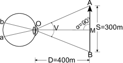
Figure 1: Effect of distance and angle on visibility

II-B1 Relative Position of the Lens and the Target

The perceived visibility of a target object mainly depends on the relative position the viewing lens and the target. For a specific target, the visibility varies with the change of distance and angle between the lens and the target.

Distance: If the distance between a target $T$ and a lens increases, the perceived size of $T$ becomes smaller. This is because the visual angle imposed by an object decreases with the increase of the distance between that object and the viewer. As shown in Fig. 1, $AB$ is a target object of length $S$ and the position of a lens is $O$. When the midpoint of $AB$ is at an orthogonal distance $D$ from $O$, the visual angle $V$ is calculated using the following formula [14],

$$V=2arctan(\frac{S}{2D})$$ (1)

Angle: The perceived size of a target $T$ depends on the angle $\alpha$ between the lens and $T$ [15]. If an object is viewed from an oblique angle, the perceived size of that object becomes smaller than the original size. For the equidistant positions of the lens from $T$, the visual angle $V$ varies for different values of $\alpha$. Let $AB$ be a line of length $S$. A line $\overline{qm}$ connecting a point $q$ and the midpoint $m$ of $AB$, creates an angle $\alpha$ with $AB$. If $\alpha=90^{o}$, the perceived size of $AB$ from a nominal distance is same as the original length, $S$. Otherwise, according to the concept of oblique projection [15], the perceived length $S_{\alpha}$ of $AB$ from $q$ is

$$S_{\alpha}=\frac{\displaystyle\alpha}{\displaystyle 90^{o}}\times S$$ (2)

Thus, if we consider the effects of both distance and angle between the target and the lens, the visual angle $V$ can be expressed as $V=2arctan(\frac{S_{\alpha}}{2D})$. In Fig. 1, the visibility of the target $AB$ of length $S$ is the visual angle $V$ imposed at the lens $O$. As in this case $\alpha=90^{o}$, so the visual angle $V$ is $2arctan(\frac{\displaystyle 300m}{\displaystyle 2\times 400m})=41.11^{o}$. If $\alpha=45^{o}$, then $V$ is $2arctan(\frac{\displaystyle 150m}{\displaystyle 2\times 400m})=21.23^{o}$.

Besides the relative position of the lens, the visibility of a target is also affected by the presence of obstacles.

II-B2 Obstacles

To show the effect of obstacles on the visibility, we first define the term point to point visibility.

Definition II.2

Point to point visibility. Given two points $p,p^{\prime}$ and a set $O$ of obstacles in a space, $p$ and $p^{\prime}$ are visible to each other if and only if the straight line connecting them, $\overline{pp^{\prime}}$, does not cut through any obstacle, i.e., $\forall o\in O,$ $\overline{pp^{\prime}}\cap o=\oslash$.

Based on the definition of point to point visibility, we formally define the obstructed region as:

Definition II.3

Obstructed region. Given a set $O$ of obstacles, a bounded region $R$, and a target $T$, the obstructed region is the set of points where for each point $p$, (i) $p$ is in $R$ and (ii) $p$ is not point to point visible to all points of $T$.

The obstructed region contains viewpoints from where the target object is not completely visible. Thus, we only need to measure the visibility for the viewpoints residing outside the obstructed region that form the visible region, and assign colors to these viewpoints of the visible region according to the defined visibility measure (i.e., visual angle).

III Constructing a VCM

To construct a VCM for a given target $T$, we need to determine the visibility of $T$ from all discrete points in the surrounding space $\mathbb{\Re}$ in the presence of a set $O$ of obstacles. We represent visibility of each point $\textsc{x}\in\mathbb{\Re}$ with a color $c_{\textsc{x}}$, which is proportional to the visibility of $T$ from x. We use the terms visibility measure and color interchangeably.

One naïve approach to compute a VCM is to compute visibility of $T$ from every single viewpoint $\textsc{x}\in\mathbb{\Re}$. Depending on how finely we discretize the space $\mathbb{\Re}$, there can be a large number of points, making the process prohibitively expensive. The high overhead of this naïve approach comes due to the expensive visibility computation from a large number of points and expensive I/O operations to retrieve a large collection of obstacles from a spatial database.

To address these problems, we propose an efficient solution to construct a VCM. The key insights of our solution come from the following two observations. First, human eye cannot visually differentiate a target from viewpoints in close proximity of each other, which eliminates the necessity of computing visibility for all viewpoints in the surrounding space. Second, in most cases, only a small subset of obstacles affect visibility of the target, and thus retrieval of all obstacles is redundant. Such redundancy can be avoided by using various indexing techniques.

In the rest of the section, we describe how we exploit these observations and propose an efficient approach to compute a VCM with reduced computational and I/O overhead. Our approach consists of three steps:

1. First, we partition the space into several equi-visible cells in the absence of obstacles exploiting the limitations of human vision. This enables us to compute one single visibility measure for each cell. This significantly reduces computational overhead in contrast to computing the color of each discrete viewpoint (Section III-A).

2. Second, we compute the effect of obstacles and divide the surrounding space into a set of visible regions such that the target is completely visible from a viewpoint if and only if it is within a visible region. To reduce the I/O overhead, we index all obstacles and incrementally retrieve only the potential obstacles that can affect the visibility of the target (Section III-B).

3. Finally, we join colors computed in the first step (that ignores obstacles) and visible regions computed in the second step to compute a VCM, i.e., colors of different parts of the space in the presence of obstacles. To reduce I/O overhead of retrieving results from the first two steps, we employ various indexes (Section III-C).

For ease of explanation, we assume a 2D space and a target with the shape of line in the subsequent sections. However, our approach is applicable to any target shapes in 2D and 3D spaces. Table I lists the notations that we use.

TABLE I: Notations used and their meanings

Notation	Meaning
$T$	The target object.
$O$	A set of b obstacles $O$=$\{o_{1},o_{2},\dots,o_{b}\}$.
$V$	The visual angle imposed in a lens by $T$.
$\mu$	The angular resolution of a lens.
$\alpha$	The angle between $T$ and the line connecting the lens and the midpoint of $T$.

III-A Partitioning Space into Equi-visible Cells

As mentioned before, the ability of a human eye (or a lens) to distinguish the variation of small details of a target $T$ of size $S$ is limited by its angular resolution $\mu$. To exploit this observation, we partition the space into a set $\zeta$ of $n$ equi-visible cells {$\zeta_{1},\zeta_{2},\dots,\zeta_{n}$}. Each cell $\zeta_{i}$ is constructed in a way so that the deviation in visibility of $T$ from the viewpoints inside a cell, measured as visual angle $V$, is not visually perceivable. Hence for any two points $p,p^{\prime}\in\zeta_{i}$, visibility from $p$ and $p^{\prime}$ is perceived as same if,

$$|V_{p}-V_{p^{\prime}}|\operatornamewithlimits{}_{p,p^{\prime}\in\zeta_{i}}\leq\mu\vspace{-3mm}$$ (3)

Note that visibility is a symmetric measure: visibility of a target at location $p$ from a viewer (i.e., the lens) at location $q$ is the same as that of a target at $q$ from location $p$. Thus, visibility of a target $T$ from the surrounding space is the same as visibility of the space from $T$’s location. Therefore, in computing visibility of $T$ from the space, we consider the viewer at the target’s location and compute visibility of the space from that location.

Since the value of visual angle depends on the distance and angle between the lens and the target, the partitioning is done in two steps: distance based partition and angle based partition.

III-A1 Distance Based Partition

As the perceived size of $T$ varies with the change of distance between $T$ and the viewer’s location, our aim is to find a set $D$ of $m$ distances, $D=\{d_{0},d_{1},\dots,d_{m-1}\}$, where for each pair of points $p,p^{\prime}$ between $d_{i}$ and $d_{i+1}$, $0\leq i<m-2$, the variation of the perceived visibility from $p$ and $p^{\prime}$ is less than or equal to the angular resolution $\mu$. Note that, since visibility varies as $\alpha$ deviates from $90^{o}$ (as explained in Section II-B1), we set $\alpha=90^{o}$ as the default value for the distance based partitioning.

Partitioning starts from the near point distance $d_{0}$, as a lens cannot focus on any object that is nearer than $d_{0}$ [16]. Initially, the visual angle $V_{0}$ from the distance $d_{0}$ is calculated using Equation 1. Then, starting from $V_{0}$, the value of the visual angle is decreased by the amount of $\mu$ at each step and the corresponding $d_{i}$ is calculated. When the imposed visual angle from a distance $d_{m-1}$ is less than $\mu$, the distance based partitioning process terminates as for any point farther than $d_{m-1}$ (i.e., $d_{max}$), the perceived visibility is indistinguishable to the viewing lens. So, we have a set $\{d_{0},d_{1},\dots,d_{m-1}\}$ of distances where every range $<d_{i},d_{i+1}>$ is a distance based partition. Fig. 2 shows the distance based partitions for a target $T$, where $d_{0}$ is the near point distance and the distance based partitions are $<d_{0},d_{1}>$, $<d_{1},d_{2}>$, and so on.

At this stage, we assign a single color for every distance based partition $<d_{i},d_{i+1}>$. However, every point in a distance based partition does not perceive the same visibility of the target, e.g., two viewpoints at a same distance partition may have different perceived visibility due to different viewing angles. Thus, in the next section we incorporate the effect of viewing angle and partition the space into equi-visible cells.

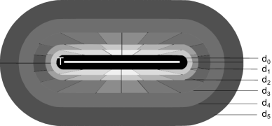
Figure 2: Partitioning based on distance and angle

III-A2 Angle Based Partition

For each distance based partition $<d_{i},d_{i+1}>$, $0\leq i<m-2$, we get $l_{i}$ numbers of angle based partitions $<\gamma_{i,j},\gamma_{i,j+1}>$, $0\leq j<l_{i}-2$, where the value of $l_{i}$ is different for each distance based partition. The visibility of every point of a partition $<d_{i},d_{i+1},\gamma_{i,j},\gamma_{i,j+1}>$ is considered as the same. We call such a partition an equi-visible cell (or, just cell in short).

As the change in perceived length due to change in $\alpha$ is symmetric with respect to both the parallel and normal axes of the object plane, we compute the angle based partitions only for the first quadrant. The partitions in other quadrants are then obtained by reflecting the partitions of the first quadrant. The procedure of angle based partitioning is as follows:

(i) For each distance based partition $<d_{i},d_{i+1}>$, the angle based partitioning starts by initializing $\alpha_{0}=90^{o}$, $\gamma_{i,0}=90^{o}$, and $S_{0}=S$, where the size of $T$ is $S$. The visual angle $V_{0}$ is calculated for $\alpha_{0}$ using Equation 1 where $D=d_{i}^{\prime}$. Here $d_{i}^{\prime}$ is the average value of distances $d_{i}$ and $d_{i+1}$, i.e., $d_{i}^{\prime}=(d_{i}+d_{i+1})/2$.

(ii) At each step $j$ of the angle based partitioning for $<d_{i},d_{i+1}>$, the perceived size $S_{j}$ is calculated for visual angle $V_{j}=V_{j-1}-\mu$ and distance $d_{i}^{\prime}$ using Equation 1, where $j\geq 1$, e.g., $S_{1}=2D\times tan\frac{V_{1}}{2}$, for $j=1$. The angle $\alpha_{j}$, for which $S_{j}$ is perceived, is computed using Equation 2, e.g., $\alpha_{1}=\frac{\displaystyle S_{1}\times 90^{o}}{\displaystyle S_{0}}$, for $j=1$. The visual angle $V_{j}$ is obtained for the change in $\gamma_{i,j-1}$ by the amount of $\alpha_{j}$, so $\gamma_{i,j}$ is updated as $\gamma_{i,j-1}-\alpha_{j}$. Thus we get an angle based partition $<\gamma_{i,j-1},\gamma_{i,j}>$ for $<d_{i},d_{i+1}>$ at each step.

(iii) When the perceived visual angle $V_{j}<\mu$, the angle based partitioning process for a distance based partition terminates.

The above process is repeated for each distance based partition and finally we get the set $\zeta=\{\zeta_{1},\zeta_{2},\dots,\zeta_{n}\}$ of $n$ cells where $n=m\times l_{i}$, $0\leq i<m-1$. Fig. 2 shows the angle-based partitions for three distance-based partitions $<d_{0},d_{1}>$, $<d_{1},d_{2}>$, and $<d_{2},d_{3}>$ for a target object $T$.

After both partitioning steps are done, we compute visibility (i.e., color) of each cell. Since all viewpoints within a cell have the same visibility, we assign the color of the entire cell as the visibility of the center of the cell to the target $T$.

Note that we have not considered the effects of obstacles yet. A caveat of this is that in the presence of obstacles, the target $T$ may not be visible from an entire cell or parts of a cell even if the cell is assigned a good visibility value. We address this next by considering the effect of obstacles.

III-B Computing the Effects of Obstacles

Given a target object $T$ and a set $O$ of obstacles, we would like to determine the set $S$ of visible regions surrounding $T$ such that $T$ is completely visible from a viewpoint $q$ if and only if $q$ is inside a visible region.

A naïve approach to determine the effects of obstacles is to retrieve all obstacles of $O$ and calculate the corresponding changes in the visibility. But this approach is prohibitively costly in terms of both I/O and computation, especially in the presence of a large number of obstacles. Moreover, considering all obstacles in the database is wasteful as only a relatively small number of obstacles around $T$ affect visibility. To efficiently retrieve this small number of obstacles around $T$, we index all obstacles in an R*-tree [17], a variation of R-tree [18]. An R*-tree consists of a hierarchy of Minimum Bounding Rectangles (MBRs), where each MBR corresponds to a tree node and bounds all the MBRs in its sub-tree. Data objects (obstacles, in our case) are stored in leaf nodes.

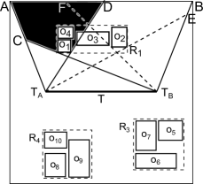
(a)

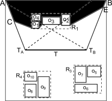
(b)

Figure 3: Visible region construction

A recent work [10] has developed a technique to determine the obstacles that affect the visibility of the target from a specific viewpoint. On the contrary, we need to compute the visible region of the whole space instead of a specific viewpoint with respect to a target. Thus, we cannot adopt the computation of the visible region from [10]. Our approach to compute the visible region in the presence of large number of obstacles is as follows.

Initially the set $V_{R}$ of visible regions contains the region of $R$ that is covered only by the field of view (FOV) with respect to the target $T$. As shown in Fig. 3a, $V_{R}$ is the region bounded by the points $T_{A}$, $T_{B}$, $A$, and $B$ where $T_{A}$ and $T_{B}$ are the corner points of $T$. Here, FOV=$120^{o}$, the usual FOV of the human eye [19]. Initially, the set $O_{R}$ of obstructed regions is the region of $R$ that is outside the FOV. As $T$ cannot be viewed from the region outside the FOV, the obstacles residing in this region is discarded from consideration.

Next, we refine the set $V_{R}$ and the set $O_{R}$ by considering one obstacle at a time. The obstacle retrieval starts from the root node of the R*-tree. Only the nodes that intersect with a region in $V_{R}$ are incrementally retrieved from the R*-tree according to their non-decreasing distances from $T$. If the retrieved node is an MBR, its elements are further discovered. For example, in Fig. 3a, when the MBR $R_{1}$ is accessed, its elements $o_{1},o_{2},o_{3}$, and $o_{4}$ are further discovered. If the retrieved node is an obstacle $o$, the regions in $V_{R}$ and $O_{R}$ are updated according to the effect of $o$. We term the effect of a single obstacle $o$ on visibility as the shadow of $o$, $W_{o}$.

Definition III.1

Shadow of an obstacle $o$, $W_{o}$. $W_{o}$ is the region formed by the set of points $P$, where for any point $p$ of $P$, there is at least a point $t_{p}$ on $T$ such that the line segment joining $t_{p}$ and $p$ either intersects or touches $o$.

From each point $p$ of the $W_{o}$, $T$ is either completely or partially obstructed. The boundary of a shadow $W_{o}$ contains exactly two straight lines, which are tangents between the obstacle and the target. If these lines are rays, not the line segments that meet each other, then the region $W_{o}$ is unbounded. If $W_{o}$ is unbounded, we consider only the portion that is bounded by the given region $R$. In Fig. 3a, The shadow of $o_{1}$ is $W_{o_{1}}$ (shown with black shade), the region bounded by $o_{1}$ and the points $A,C,$ and $D$.

While updating the $V_{R}$ and $O_{R}$ for the shadow of a retrieved obstacle, there are three cases to be considered:

(i) If the obstacle $o$ or its shadow $W_{o}$ does not overlap with any obstructed region of $O_{R}$, we exclude $W_{o}$ from $V_{R}$ and include it in $O_{R}$. In Fig. 3a, obstacle $o_{1}$ is the first obstacle retrieved according to its non-decreasing distance from $T$. As there is no other obstructed region to be overlapped with $o_{1}$ or its shadow $W_{o_{1}}$ (shown as the black region), $W_{o_{1}}$ is now excluded from $V_{R}$ and included in $O_{R}$.

(ii) If $o$ or $W_{o}$ overlaps with one or more obstructed regions of $O_{R}$, we combine these regions and $W_{o}$ into a single obstructed region and discard this region from $V_{R}$. Let $N$ be the set of $W_{o}$ and the obstructed regions that overlap with $W_{o}$. To combine the regions in $N$, we determine the leftmost tangent line $l$ and the rightmost tangent line $r$ of all the shadows of $N$ such that the region bounded by $l$, $r$ and the union of the shadows of $N$ enclose all the obstructed regions of $N$. This shadow resembles the combined effect of the obstacles that are included in $N$. We replace the regions of $N$ from $O_{R}$ with this combined region and discard it from $V_{R}$. As an example, in Fig. 3a, the shadow $W_{o_{2}}$ (shown with dotted lines) of the next retrieved obstacle $o_{2}$ overlaps with the existing obstructed region (shown with black shade). Here, the leftmost tangent line and the rightmost tangent line of these obstructed regions are the line connecting $o_{1}$, $C$ and the line connecting $o_{2}$, $E$, respectively. The region enclosed by these two lines and the union of the shadows is discarded from $V_{R}$. Similarly, the next retrieved obstacle $o_{3}$ overlaps with $O_{R}$. The shadows combined for obstacle $o_{1}$, $o_{2}$, and $o_{3}$ is shown in black shade in Fig. 3b, where the shadow of $o_{3}$ is shown with dotted lines.

(iii) If $o$ is entirely inside any obstructed region, it will not contribute to the visibility. So we discard $o$ from consideration. In Fig. 3b, the effect of obstacle $o_{4}$ is not calculated as it is entirely inside the current obstructed region.

Note that, the visible region includes viewpoints from where the target is entirely visible. This approach is suitable for applications like placement of billboards, where partial visibility of the target from a viewpoint does not make sense. There can be some applications that require finding the viewpoints from where a target is partially visible. We leave computing the partial visible viewpoints as the scope of the future study.

III-C Merging Cells with Visible Regions

In the final step of producing a VCM, we combine colors computed in the first step (that ignores obstacles) and visible regions computed in the second step to compute color of each cell in the presence of obstacles. Intuitively, all obstructed regions are assigned color zero (representing zero visibility), while all visible regions are assigned colors from their corresponding cells. This requires taking intersection (spatial join) of all cells and visible regions.

The above process can be expensive for two reasons. First, visible regions are usually irregular polygons and intersecting them with cells incurs high computational overhead due to the complex shapes of the polygons. We address this by storing each polygon as a set of regular shapes (rectangles) with a quad-tree [20]. Second, the number of cells can be quite large and intersecting visible regions with all cells can be expensive. We address this by indexing the cells in an R*-tree and intersecting each visible region only with its overlapping cells. We describe these optimizations below.

III-C1 Indexing Visible Regions

We index visible (and obstructed) regions in a 2D (3D) space with a quad-tree (octree). Quad-trees (Octrees) partition a 2D (3D) space by recursively subdividing it into four quadrants (eight octants) or blocks. Initially the whole space is represented with a single quad-tree block. In the visible region computation phase, when a region is obstructed due to a retrieved obstacle, a quad-tree block is partitioned into four equal blocks if it intersects with the obstructed region. The partitioning continues until (i) a quad-tree block is completely visible, or (ii) completely obstructed, or (iii) the size of a block is below a threshold value $\vartheta$. The threshold size is determined from the partitioning phase. If the set of the boundary points of an equivalence cell $\zeta_{i}$ is $\beta_{\zeta_{i}}$, the minimum distance between any two opposite boundaries over all cells is specified as $\vartheta$, i.e.,

$$\vartheta=\operatornamewithlimits{arg\,min}_{\zeta_{i},1\leq i\leq n}(\operatornamewithlimits{arg\,min}_{p,p^{\prime}\in\beta_{\zeta_{i}}}(mindist(p,p^{\prime}))\vspace{-3.6mm}$$

where, points $p,p^{\prime}\in\beta_{\zeta_{i}}$ are points of opposite boundaries.

As $\vartheta$ is the minimum size of a cell obtained in the partitioning phase and the deviation in the perceived visibility for a block-size less than $\vartheta$ is not distinguishable due to angular resolution of a lens, dividing a quad-tree block into size smaller than $\vartheta$ for more accuracy is redundant.

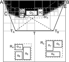
(a)

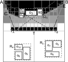
(b)

Figure 4: Construction of visibility color map

Fig. 4a shows the quad-tree of the obstructed region (black blocks) and visible region (white blocks inside FOV). After the quad-tree is constructed, we start assigning color to each of its blocks. We get the VCM after all the blocks are assigned colors. The blocks that fall in the obstructed region are assigned zero visibility. The remaining blocks (i.e., visible region) are assigned colors based on the colors of their corresponding cells, as described next.

III-C2 Indexing Cells and Constructing VCM

For each quad-tree block with unassigned color, we need to find all overlapping cells in order to find its color. To expedite this process, we index cells with an R*-tree that we call the color-tree. Leaf nodes in the color-tree represent cells and non-leaf nodes represent MBRs containing the shapes of their children nodes. Then, for each quad-tree block, we run a range query on the color-tree. The color for an unassigned quad-tree block is obtained by calculating the intersection of the spatial region of that block and the cells from the color-tree. If the quad-tree block intersects with a single cell of the color partition, the block is assigned the color of that cell. If a quad-tree block intersects with multiple cells, in a 2D (3D) space we further divide that block into four (eight) equal blocks. The division is continued until either a block intersects with a single cell or the size of a block is below the threshold value $\vartheta$ (Section III-C1). The process terminates when all quad-tree blocks of the visible region are colored according to the visibility measure. Fig. 4b shows the resulting VCM constructed by combining the color partitions of Fig. 2 and the quad-tree of Fig. 4a.

The steps of constructing a VCM are shown in Algorithm 1. Lines 1.6-1.9 shows accessing the color-tree nodes. If an accessed node is an MBR, its elements are further discovered from the color-tree (Lines 1.21-1.22). If the accessed node is a leaf node, the quad-tree nodes that are not colored yet and intersects with this node are either colored or partitioned further (Lines 1.15-1.20). Finally, the colored quad-tree is returned as the complete VCM.

0.1 Initialize $Q$ to an empty queue;

0.2 Initialize $L$ to an empty list;

0.3 $node\leftarrow{CTree.root}$; $end\leftarrow$ false;

0.4

0.5$L\leftarrow Get\_unassigned\_quad_{\_}leaf(Qtree,FOV)$;

0.6

0.7while $node\neq$ empty and $end$ = false do

0.8       for each element $n_{e}$ of $node$ do

0.9             if Inside_visibility_region($n_{e}$) = true then

0.10                   $Enqueue(Q,n_{e})$;

0.11                  

0.12            

0.13      

0.14      $continue\leftarrow$ true;

0.15       while $continue$ = true do

0.16             $continue\leftarrow$ false; $node\leftarrow Dequeue(Q)$;

0.17             if $node$ = empty or $L$ = empty then

0.18                   $end\leftarrow$ true;

0.19                  

0.20             else if $node$ is a data object then

0.21                   Initialize $Still\_unassigned\_quads$ to an empty list;

0.22                   for each element $L_{i}$ of $L$ do

0.23                         $Still\_unassigned\_quads\leftarrow insert(Divide\_and\_color(L_{i},node,\vartheta))$;

0.24                        

0.25                  $L\leftarrow Still\_unassigned\_quads$;

0.26                  

0.27                  $continue\leftarrow$ true;

0.28                  

0.29             else

0.30                   $node\leftarrow$ child($node$);

0.31                  

0.32            

0.33      

return $Qtree$;

Algorithm 1 ConstructVCM($T,FOV,\vartheta,Qtree,CTree$)

Since the color partition results in complex shaped cells (e.g., curves), it is computationally expensive to combine these shapes with the quad-tree blocks of visible region. Thus, we propose two approaches to approximate color partition cells.

IV Extensions

In this section, we discuss a few extensions to our basic algorithm described in the previous section.

IV-A Approximation of Partitions

The algorithm in the previous section partitions the space according to the relative distance and angle between the lens and the target. Based on these parameters, the cells are bounded by arcs and straight lines. To construct the VCM, we need to compute the intersection of these cells with the quad-tree blocks. The process is computationally expensive due to the complex shape of the cells and the target.

To address this, we introduce two approximations that reduce the computational overhead at the cost of small bounded errors: (i) minimum bounding rectangle (MBR) of a cell and (ii) tangents of the arcs of a cell. For the ease of explanation we analyze errors for targets with regular shapes, e.g., lines without loss of generality. For such targets, the complex shaped partitions are bounded by two arcs and two straight lines. Here we discuss the approximations of color partitions and the maximum error resulting from these approximations.

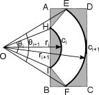
(a)

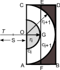
(b)

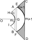
(c)

Figure 5: Approximating a cell using MBR and tangents

MBR Approximation

An approach to approximate the curves of a cell is to enclose the cell using its MBR where the area covered by the cell is approximated by the area covered by the enclosing MBR. This is illustrated in Fig. 5a, where a cell consists of two concentric arcs $c_{i}$ and $c_{i+1}$ (centered at a corner $O$ of the target) of radius $r_{i}$ and $r_{i+1}$, respectively. $ABCD$ is the MBR of this cell. Let $c_{i}$ and $c_{i+1}$ create $\theta_{i}$ and $\theta_{i+1}$ angles (in degrees) at the center respectively. We denote the area of the MBR as $A_{r}$. So the area bounded by the cell, $A_{p}$ is $(\frac{\theta_{i+1}}{360}\times\pi{r_{i+1}}^{2})-(\frac{\theta_{i}}{360}\times\pi{r_{i}}^{2})$. Hence the area that gets wrong color due to this MBR approximation is $A_{r}-A_{p}$ (shaded region in Fig. 5a).

Error Bound Analysis. For targets with regular shapes such as lines (Fig. 2), the largest cell that can yield the maximum possible error consists of two half circles centered at a corner point of the target. Hence we formulate the maximum error bound by referring to Fig. 5b. Here, we want to approximate the area of a cell $p_{i}$ bounded by two half circles $c_{i}$ and $c_{i+1}$ centered at $O$, a corner point of target $T$ of length $S$. Here, $c_{i}$ and $c_{i+1}$ belong to distance based partition $d_{i}$ and $d_{i+1}$, respectively. We approximate $p_{i}$ by taking its MBR, $ABCD$. So, the darkly shaded region is wrongly colored for MBR approximation. The lightly shaded region is wrongly colored too, but it is considered for distance based partition $<d_{i-1},d_{i}>$ i.e., for cell $p_{i-1}$. As the total error is calculated incrementally for each cell, so the error for this lightly shaded region is calculated only once for the cell $p_{i-1}$. Let, $r_{i}$ and $r_{i+1}$ be the radii of $c_{i}$ and $c_{i+1}$, respectively. Hence, the width of cell $p_{i}$ is $r_{i+1}-r_{i}$. The farthest distance from $O$ to any point of the MBR is $\Delta r=\sqrt{2}\times r_{i+1}$. So the points of the MBR that fall within the distance $r_{i+1}$ and $\sqrt{2}\times r_{i+1}$ from point $O$, get wrongly colored with the $p_{i}$’s color. From Equation 1 we get that the width of the distance based partitions increase with the increase of the distance between the target and the partition. So the maximum number of distance based partitions in $d_{i+1}$ that can be wrongly colored is $n=\frac{\Delta r-r_{i+1}}{r_{i+1}-r_{i}}$.

For each distance based partition, corresponding angle based partitions are calculated by taking the angle from the midpoint of the target. So only the angle based partitions that fall within the range ($\arctan\frac{r_{i+1}}{S/2}$, $-\arctan\frac{r_{i+1}}{S/2}$) can lie in the darkly shaded region. Let there are $a_{i}$ such angle based partitions in total. As the difference in visual angle in consecutive partitions is $\mu$, the maximum variation in color for a cell is, $\Delta c_{m_{i}}=n\times a_{i}\times\mu$. So when the total number of partitions is $k$ and the area of $i$th cell is $A_{i}$, the total error in coloring is:

$$E_{MBR}=\sum_{i=1}^{k}\Delta c_{m_{i}}\times A_{i}$$ (4)

Tangential Approximation

We obtain another approximation approach by taking tangents in the midpoints of the two arcs that encloses a cell. Here the area enclosed by two arcs is approximated by the area enclosed by the tangents at their midpoints. In Fig. 5c the cell is bounded by arcs $c_{i}$ and $c_{i+1}$ centered at a corner $O$ of the target $T$. We take two tangents $AB$ and $CD$ of $c_{i}$ and $c_{i+1}$ at their midpoints $m_{i}$ and $m_{i+1}$, respectively. So we want to approximate the area bounded by these two arcs with the trapezoid $ABDC$. Let, the angles created at $O$ by $c_{i}$ and $c_{i+1}$ are $\theta_{i}$ and $\theta_{i+1}$ (in degrees). If we color the trapezoid $ABDC$ instead of the cell, the region that gets wrong color is the shaded region of Fig. 5c. Let the area of the trapezoid $ABDC$ be $A_{t_{1}}$, the radius of $c_{i+1}$ is $r_{i+1}$, the midpoint of $\overline{EF}$ is $G$, and the length of $\overline{OG}$ is $x$. Then the length of $\overline{EG}$ is $\sqrt{{r_{i+1}}^{2}-x^{2}}$. The area of the segment bounded by $\overline{EG}$ and $c_{i+1}$, $A_{c}$ is $(\frac{\theta_{i+1}}{360}\times\pi{r_{i+1}}^{2})-x\times\sqrt{{r_{i+1}}^{2}-x^{2}}$. If the area of the trapezoid $ABFE$ is $A_{t_{2}}$, then the area of the shaded region $A_{e}$ is $A_{t_{1}}-A_{c}-A_{t_{2}}$. According to this tangential approximation the region that is wrongly colored due to cell $HIFE$ is this shaded region with area $A_{e}$.

Error Bound Analysis. In case of MBR approximation the cell bounded by two half circles is approximated by an enclosing MBR, while for tangential approximation that cell is approximated by a rectangle bounded by the tangents of those two half circles. Referring to Fig. 5b, the cell bounded by arcs $c_{i}$ and $c_{i+1}$ is approximated by rectangle $ABDC$ and rectangle $FBDE$ for MBR and tangential approaches, respectively. In this figure, $G$ is the midpoint of $c_{i}$ and the farthest distance from $G$ to any point inside the approximated cell is $\Delta r=\sqrt{r_{i+1}^{2}+(r_{i+1}-r_{i})^{2}}$. So the points inside the darkly shaded region are wrongly colored. As the width of the distance based partitions relates inversely to the distance between the target and the partition (Equation 1), the maximum number of distance based partitions in $d_{i+1}$ that can be wrongly colored is $n=\frac{\Delta r-r_{i+1}}{r_{i+1}-r_{i}}$. In case of angle based partitioning, only the angle based partitions that fall within the range ($\arctan\frac{r_{i+1}}{S/2+r_{i}}$, $-\arctan\frac{r_{i+1}}{S/2+r_{i}}$) can lie in the darkly shaded region inside the rectangle $EFBD$. Let there are $a_{i}$ such angle based partitions in total. As the difference in visual angle in consecutive partitions is $\mu$, the maximum variation in color for a cell is, $\Delta c_{t_{i}}=n\times a_{i}\times\mu$. So when the total number of partitions is $k$ and the area of $i$th cell is $A_{i}$, the total error is:

$$E_{Tangent}=\sum_{i=1}^{k}\Delta c_{t_{i}}\times A_{i}$$ (5)

In the above sections, we discussed our approach to construct target-centric visibility color map. The approach is same for the viewer-centric visibility color map with an additional initialization step. The details of viewer-centric VCM is discussed below.

IV-B Viewer-centric VCM

A viewer-centric VCM is constructed by calculating the visibility of the surrounding space for a given viewpoint $q$ and a set $O$ of obstacles. Unlike the target-centric VCM where a particular target is specified, in case of the viewer-centric VCM, a particular viewer position is specified. To measure the visibility using Equation 1 and Equation 2 in case of the viewer-centric VCM, first we need an initial value of the size $S$ of a target from the given information.

The visibility of any point farther than a distance $d_{max}$ is not visually distinguishable if the perceived visual angle of that point is less than the angular resolution $\mu$ from $q$ (Section III-A1). Based on this fact, we assume a circular region $R$ of radius $d_{max}$ centered at $q$ to construct the VCM of $R$ only, as the visibility of the points outside $R$ are not distinguishable by a viewer at $q$. Using Equation 1, we calculate the size $S$ of a target for which visual angle $V=\mu$ is perceived at distance $d_{max}$. After taking $S$ as the size of the target, the steps of our approach discussed for the target-centric VCM is applied in the same manner to construct the viewer-centric VCM.

IV-C Incremental Processing

During the computation of the VCM, we have assumed that the field of view (FOV), i.e., the orientation of the viewpoint or the target is fixed. At a particular orientation or gaze direction, only the extents of the space that is inside the FOV, is visible. With the change in viewing direction, some areas that were previously outside the FOV become visible. In this case, we do not need to compute the full VCM each time, rather we can incrementally construct the VCM by computing for the newly visible parts only.

In the incremental process, the only information that varies is the gaze direction. So, as a preprocessing step we can construct the color-tree and the visible region quad-tree in the above discussed method by considering the FOV as $360^{o}$. A VCM is then constructed by combining the color-tree and the quad-tree for a particular gaze direction. When the gaze direction changes, only the uncolored quad-tree blocks that are now included in the visibility region are assigned colors. Hence the color-tree and the quad-tree are constructed only once. This reduces the computational complexity to a great extent by avoiding same calculations repetitively. From our conducted experiments we also observe that the processing time required to combine the color-tree and the quad-tree is much smaller than the processing time required to construct the visibility region quad-tree for a dataset of densely distributed large number of obstacles (Section 8 and  V-D1). So for such cases we can significantly improve the performance of our proposed solution by adopting the preprocessing strategy.

V Experimental Evaluation

We evaluate the performance of our proposed algorithm for constructing the visibility color map (VCM) with two real datasets. Specifically, at first we compare our approach with a baseline approach that approximates the total space into a regular grid and compute visibility from the midpoint of each grid cell, and then we compare our two approximation algorithms, i.e., MBR approximation ($VCM_{M}$) and tangential approximation ($VCM_{T}$) with the exact method ($VCM_{E}$). The algorithms are implemented in C++ and the experiments are conducted on a core i5 2.40 GHz PC with 3GB RAM, running Microsoft Windows 7.

V-A Experimental Setup

Our experiments are based on two real datasets: (1) British representing 5985 data objects obtained from British ordnance survey and (2) Boston representing 130,043 data objects in Boston downtown. In both datasets, objects are represented as 3D rectangles that are used as obstacles in our experiments. For both datasets, we normalize the dataspace into a span of $10,000\times 10,000$ square units. For 2D, the datasets are normalized by considering $z$-axis value as 0. All obstacles are indexed by an R*-tree, with the disk page size fixed at 1KB.

TABLE II: Parameters

Parameter	Range	Default
Angular Resolution ($\mu$)	1, 2, 4, 8, 16	4
Minimum Block Size ($\vartheta$)	1, 2, 4, 8, 16	1
Query Space Area ($A_{Q}$)	0.05, 0.10, 0.15, 0.2, 0.25	0.15
Field of View ($FOV$)	60, 120, 180, 240, 300, 360	120
Length of Target ($L_{T}$)	0.05, 0.10, 0.15, 0.2, 0.25	0.15
Dataset Size ($D_{S}$)	5k, 10k, 15k, 20k, 25k

The experiments investigate the performance of the proposed solutions by varying five parameters: (i) angular resolution ($\mu$) in arcminutes, (ii) the threshold of the quad-tree block size ($\vartheta$) as the multiple of the calculated minimum size (as explained in Section III-C1), (iii) the area of the space ($A_{Q}$) as the percentage of the total area, (iv) field of view ($FOV$) in degrees, and (v) the length of the target ($L_{T}$) as the percentage of the length of total dataspace. We have also varied the dataset size using both Uniform and Zipf distribution of the obstacles. The range and default value of each parameter are listed in Table II. In concordance with human vision, the default values of $\mu$ and $FOV$ are set as $4$ arcminutes [11] and $120^{o}$ [19], respectively. The minimum threshold of quad-tree block size as calculated in Section III-C1 is used as the default value of $\vartheta$. The default values of other parameters are set to their median values.

The performance metrics that are used in our experiments are: (i) the total processing time, (ii) the total I/O cost, and (iii) the error introduced by the two approximations: $VCM_{M}$ and $VCM_{T}$. We calculate the approximation error as the deviation from the color map of $VCM_{E}$, i.e.,

$$error=\frac{\sum_{i}(c_{e_{i}}\times A_{i}-c_{a_{i}}\times A_{i})}{\sum_{i}c_{e_{i}}\times A_{i}}$$ (6)

Here $c_{e_{i}}$ is the color of $i$th cell in $VCM_{E}$, $c_{a_{i}}$ is the color of $i$th cell in $VCM_{M}$ or $VCM_{T}$, and $A_{i}$ is the area of the $i$th cell.

For each experiment, we have evaluated our solution for the target at 100 random positions and reported their average performance. We have conducted extensive experiments using two datasets for both 2D and 3D spaces. Since, 2D dataspace is a subset of 3D dataspace and most of the real applications involve 3D scenario, we omit the detailed results of 2D due to the brevity of presentation.

(a) British ordnance survey

(b) Boston downtown

Figure 6: Real datasets used in the experiments

(a) British ordnance survey

(b) Boston downtown

Figure 7: Dataset distribution

V-B Comparison with the Baseline

The performance improvement of our approach over the baseline approach is measured in terms of the total processing time required for computing the VCM. In the naïve approach, we need to compute visibility of the target from infinite number of points to construct the VCM as every point in the dataspace acts as a viewpoint. Even discretizing the surrounding space into 1000 points in each dimension would give a total of $10^{9}$ points in the 3D space. We observe that the time required for such computation using British and Boston datasets are approximately 74 days and 128 days, respectively. As such naïve approach is trivial, we can further improve it by dividing the dataspace into $500\times 500\times 500$ cubic cells in 3D and choose the visibility from the middle point of each cell to represent the visibility of that entire cell. In the rest of the paper we refer to this approach as the baseline approach to construct the VCM. The comparison between the baseline approach and our proposed solution $VCM_{E}$ is presented in Table III in terms of total processing time and introduced error. In this case the parameters are set to their default values (Table II). We observe that when compared to $VCM_{E}$, for British dataset the baseline approach runs 818 times slower and introduces $30$% error, while for Boston dataset the baseline approach runs 837 times slower and introduces $32$% error.

TABLE III: Comparison with the baseline

Dataset	Baseline		$VCM_{E}$
	Total time	Error (%)	Total time
British	58hrs	30.33%	253.07s
Boston	61hrs	31.76%	245.26s

V-C Performance in 2D

In this section, we present experimental results for 2D datasets.

V-C1 Effect of $\mu$

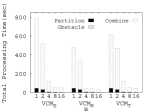
(a)

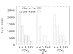
(b)

Figure 8: Effect of $\mu$ in 2D British (a-b) dataset

TABLE IV: Error in $VCM_{M}$ and $VCM_{T}$ for varying $\mu$ in 2D

Dataset	Method	Error (%)
		1	2	4	8	16
British	$VCM_{M}$	2.0	1.64	4.25	4.42	5.38
	$VCM_{T}$	0.01	0.01	0.01	3.64	3.91

In this experiment, we vary the value of $\mu$ as 1, 2, 4, 8, and 16 arcminutes and measure the total processing time and I/Os for British datasets (Fig. 8). We also present the errors resulted in the two approximations (Table  IV).

For British dataset, on average $VCM_{M}$ and $VCM_{T}$ are 65% times and 17% times faster than $VCM_{E}$, respectively. In general, with the increase in $\mu$, the cell size increases and the number of total partition in the dataspace decreases. Moreover, larger $\mu$ yields fewer branching in the visibility region quad-tree. So, with the increase in $\mu$, total processing time and I/O cost decrease rapidly for both datasets. The total I/O cost is composed of (i) cost of partitioning the total dataspace to form the color-tree, (ii) cost of retrieving obstacles to form visibility region quad-tree, and (iii) cost of combining the color-tree and quad-tree to form the VCM. As these three costs hardly differ for all three approaches, they result into similar I/O cost. On the other hand, as with the increase in $\mu$, the area of partition cells ($A_{i}$) gets larger, the estimated error increases for both $VCM_{M}$ and $VCM_{T}$ (Equation 6). The average errors introduced in $VCM_{M}$ and $VCM_{T}$ are 3.5% and 1.5%, respectively.

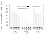
(a)

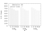
(b)

Figure 9: Effect of $\vartheta$ in 2D British (a-b)

V-C2 Effect of $\vartheta$

TABLE V: Errors in $VCM_{M}$ and $VCM_{T}$ for $\vartheta$ in 2D

Dataset	Method	Error (%)
		1	2	4	8	16
British	$VCM_{M}$	0.01	2.74	9.29	12.59	12.83
	$VCM_{T}$	0.01	0.77	4.37	6.26	7.54

In this experiment, we vary the quad-tree block size ($\vartheta$) as 1, 2, 4, 8, and 16 times of the minimum threshold of a quad-tree block. The results are presented in Fig. 9 and Table V.

For British dataset, $VCM_{M}$ is approximately 2.3 times faster than both $VCM_{T}$ and $VCM_{E}$. As explained earlier, $VCM_{M}$ and $VCM_{T}$ yield I/O costs similar to $VCM_{E}$. On average, $VCM_{M}$ and $VCM_{T}$ introduce 7.5% and 3.8% errors, respectively. These amounts of errors do not have noticeable impact on many practical applications. We observe from Equation 1 that the cells generated near the target are very small. Therefore the approximations of the cells close to the target are almost similar to the corresponding exact cells. The cell size increases with the increase of distance and a significant portion of errors is introduced for these distant cells. As the visibility of the target from distant cells is insignificant in most of the cases, the error in such cells is tolerable.

In general, with the increase in $\vartheta$, the introduced errors in $VCM_{M}$ and $VCM_{T}$ increase as a larger quad-block size approximates the cells with lesser accuracy. But with the increase in $\vartheta$, the total processing time and I/O cost reduce significantly. Hence for applications that can tolerate reduced accuracy, a large $\vartheta$ can result into better performance.

V-D Performance in 3D

In this section, we present the experimental results for 3D British and Boston datasets by varying different parameters.

TABLE VI: Errors in $VCM_{M}$ and $VCM_{T}$ for $\mu$ in 3D

Dataset	Method	Error (%)
		1	2	4	8	16
British	$VCM_{M}$	4.56	8.02	8.11	10.46	15.25
	$VCM_{T}$	4.1	7.63	7.76	8.89	13.89
Boston	$VCM_{M}$	3.31	5.03	8.02	9.12	10.05
	$VCM_{T}$	3.12	4.70	7.62	8.57	9.79

V-D1 Effect of $\mu$

In this experiment, we vary the value of $\mu$ as 1, 2, 4, 8, and 16 arcminutes and measure the total processing time and I/Os for British and Boston datasets (Fig. 10). We also present the errors resulted in the two approximation methods (Table VI).

For British dataset, on average $VCM_{M}$ and $VCM_{T}$ run only 5% and 3% faster than $VCM_{E}$, respectively. The difference in I/O cost, i.e., the number of pages accessed is also negligible among the three methods. As discussed earlier in Section III the three methods differ only in the final phase, i.e., combining the outcome of previous two steps to produce the VCM. As we consider only full visibility of the target object from a partition cell, a huge number of cells in the dataspace fall into the obstructed region. So in the final phase the three solutions perform similarly as they have to combine the same color-tree and visible region quad-tree. The average errors introduced in $VCM_{M}$ and $VCM_{T}$ are 9% and 8%, respectively.

Although the results for both British and Boston datasets follow similar pattern, Boston dataset causes much smaller I/O and computational cost. Because, in case of the densely populated Boston dataset, most of the obstacles are pruned rapidly during the visible region quad-tree formation. So there are lesser number of visibility computation and page access to construct VCM in Boston dataset. The processing time of $VCM_{M}$ is on average 8% faster than that of $VCM_{E}$ and $VCM_{T}$. The average error introduced in $VCM_{M}$ is 7%, whereas the more accurate $VCM_{T}$ yields 6% error.

The I/O costs in the obstacle retrieval phase are same in all three methods. Thus in subsequent sections, we show only the I/O cost required to combine the quad-tree and the color-tree (i.e., the final phase of constructing the VCM).

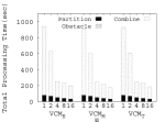
(a)

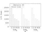
(b)

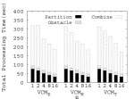
(c)

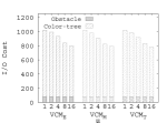
(d)

Figure 10: Effect of $\mu$ in 3D British (a-b) and Boston (c-d)

(a)

(b)

(c)

(d)

Figure 11: Effect of $\vartheta$ in 3D British (a-b) and Boston (c-d)

TABLE VII: Errors in $VCM_{M}$ and $VCM_{T}$ for $\vartheta$ in 3D

Dataset	Method	Error (%)
		1	2	4	8	16
British	$VCM_{M}$	8.11	9.31	10.15	11.83	14.96
	$VCM_{T}$	7.76	9.00	9.86	11.05	12.72
Boston	$VCM_{M}$	8.02	9.08	9.38	9.82	11.03
	$VCM_{T}$	7.62	8.82	9.06	8.98	10.29

V-D2 Effect of $\vartheta$

In this experiment, we vary the quad-tree block size $\vartheta$ as 1, 2, 4, 8, and 16 times of the minimum threshold of a quad-tree block and show the results in Fig. 11 and Table VII.

For British dataset, the computational and I/O costs are similar for all three methods, e.g., on average $VCM_{M}$ runs only 3% faster than $VCM_{E}$. Because, similar to the case of varying $\mu$, the three phases of constructing VCM differ slightly for these methods. The average error introduced in $VCM_{M}$ and $VCM_{T}$ is about 10%. The results derived from Boston dataset are similar to that of British dataset. $VCM_{M}$ runs about 3% faster than both $VCM_{E}$ and $VCM_{T}$. The average errors introduced in the approximation methods are about 9%.

As the errors introduced by two approximations show similar trends for $A_{Q}$, FOV, and $L_{T}$, we show only the total processing time and the I/O cost in the subsequent sections.

(a)

(b)

Figure 12: Effect of $A_{Q}$ in 3D British (a) and Boston (b)

(a)

(b)

Figure 13: Effect of $FOV$ in 3D British (a) and Boston (b)

V-D3 Effect of $A_{Q}$

In this experiment, we vary the query area $A_{Q}$ as 5%, 10%, 15%, 20%, and 25% of the total dataspace (Fig. 12(a)-(b)). In case of British dataset, $VCM_{M}$ and $VCM_{T}$ run 5% and 3% faster than $VCM_{E}$, respectively. For Boston dataset, $VCM_{M}$ runs 5% faster than both $VCM_{E}$ and $VCM_{T}$. The I/O cost and the total processing time increase for all three methods with the increase in $A_{Q}$, as we need to consider higher number of cells and higher number of obstacles to construct the VCM. As the I/O cost is similar for all three methods, we show only the total processing time.

V-D4 Effect of FOV

In this experiment, we vary the field of view (FOV) as 60, 120, 180, 240, 300, and 360 degrees for British and Boston datasets (Fig. 13). When FOV is set to $360^{o}$, the FOV covers the surrounding space in all directions. We observe that the processing time and I/Os increase with the increase of FOV, which is expected.

Like the previous cases, the total processing time and I/O cost are similar for all three methods. For British and Boston dataset, $VCM_{M}$ runs 3% and 4% faster than both $VCM_{E}$ and $VCM_{T}$, respectively. With the increase of FOV from 60 to 360 degrees, the total processing time of $VCM_{E}$ increases by nearly 40% and 46% for British and Boston dataset, respectively. On the other hand, the I/O costs increase 33% and 31% for British and Boston dataset, respectively.

V-D5 Effect of $L_{T}$

In this experiment, we vary the length of target $L_{T}$ as 5%, 10%, 15%, 20%, and 25% of the total length of the dataspace. In general, with the change in $L_{T}$, no significant change in performance is observed for any of the datasets (not shown).

V-D6 Effect of varying $D_{S}$

(a)

(b)

Figure 14: Effect of varying dataset size in 3D (a-b)

In this experiment we vary the number and distribution of obstacles and measure the performance of our approximation methods in terms of I/O cost, total processing time, and approximation errors. We vary $D_{S}$ as a set of 5k, 10k, 15k, 20k, and 25k obstacles while keeping the other parameters at their default values. We consider both Uniform (U) and Zipf (Z) distributions of the obstacles.

In general, as the number of obstacles increases, the area of the dataspace gets more obstructed. So during the final phase of VCM construction (i.e., combining color-tree and visible region quad-tree), computational costs and I/O costs get reduced. Consequently, the overall costs decrease with the increase in $D_{S}$ for both Uniform and Zipf distribution. In case of Uniform and Zipf distributions, as the number of obstacles is varied from 5k to 25k, the total processing time decreases nearly 40% and 20%, respectively for all three methods. On the other hand, the I/O costs decrease approximately 18% and 17% with the increase of $D_{S}$ for Uniform and Zipf distributions, respectively.

VI Related Works

The notion of visibility is actively studied in different contexts: computer graphics and visualization [4, 9] and spatial databases [1, 2, 3]. Most of these techniques consider visibility as a binary notion, i.e., a point is either visible or invisible from another point.

VI-A Visibility in Computer Graphics and Visualization

In computer graphics, the visibility map refers to a planar subdivision that encodes the visibility information, i.e., which points are mutually visible [4]. Two points are mutually visible if the straight line segment connecting these points does not intersect with any obstacle. If a scene is represented using a planar straight-line graph, a horizontal (vertical) visibility map is obtained by drawing a horizontal (vertical) straight line $l$ through each vertex $p$ of that graph until $l$ intersects an edge $e$ of the graph or extends to infinity. The edge $e$ is horizontally (vertically) visible from $p$. A large body of works [5, 6, 7, 8, 9] construct such visibility maps efficiently.

Given a collection of surfaces representing boundaries of obstacles, Tsai et al. considers visibility problem as determining the regions of space or the surfaces of obstacles that are visible to an observer [21, 22]. They model visibility as a binary notion and find the light and dark regions of a space for a point light source.

Above methods involve the computation of visible surfaces from a viewpoint and do not consider visibility factors such as angle and distance to quantify the visibility of a target object.

VI-B Visibility in Spatial Queries

Visibility problems studied in spatial databases usually involve finding the nearest object to a given query point in the presence of obstacles. In recent years, several variants of the nearest neighbor (NN) queries have been proposed that include Visible NN (VNN) query [1], Continuous Obstructed NN (CONN) query [2], and Continuous Visible NN query [3].

Nutanong et al. introduce an approach to find the NN that is visible to a query point [1]. A CNN query finds the $k$ NNs for a moving query point [23]. Gao et al. propose a variation of CNN; namely, a CONN query [2]. Given a dataset $P$, an obstacle set $O$, and a query line segment $q$ in a 2D space, a CONN query retrieves the NN of each point on $q$ according to the obstructed distance.

The aforementioned spatial queries find the nearest object in an obstructed space from a given query point where query results are ranked according to visible distances from that query point. Instead of quantifying visibility as a non-increasing function from a target to a viewpoint, they label a particular point or region as either visible or invisible. But for constructing a VCM of the entire space, such binary notion is not applicable.

Recently the concept of maximum visibility query is tossed in [10] that considers the effect of obstacles during quantifying visibility of a target object. They measure the visibility of a target from a given set of query points and rank these query points based on the visibility measured as the visible surface area of the target.

VII Conclusion

In this paper, we have proposed a technique to compute a visibility color map (VCM) that forms the basis of many real-life visibility queries in 2D and 3D spaces. A VCM quantifies the visibility of (from) a target object from (of) each viewpoint of the surrounding space and assigns colors accordingly in the presence of obstacles. Our approach exploits the limitation of a human eye or a lens to partition the space into cells in the presence of obstacles such that the target appears same from all viewpoints inside a cell.

Our proposed solution significantly outperforms the baseline approach by at least $800$ times and six orders of magnitude in terms of computational time and I/O cost, respectively for both datasets. Our conducted experiments on real 2D and 3D datasets demonstrate the efficiency of our approximations, $VCM_{M}$ and $VCM_{T}$. On average, the approximations $VCM_{M}$ and $VCM_{T}$ improve the processing time by 65% and 17% over $VCM_{E}$, respectively and require almost similar I/O costs. Both of $VCM_{M}$ and $VCM_{T}$ improve the efficiency of $VCM_{E}$ by introducing only 9% and 5% error on average.

References

- [1] S. Nutanong, E. Tanin, and R. Zhang, “Incremental evaluation of visible nearest neighbor queries,” TKDE, vol. 22, pp. 665–681, 2010.
- [2] Y. Gao and B. Zheng, “Continuous obstructed nearest neighbor queries in spatial databases,” in SIGMOD, 2009, pp. 577–590.
- [3] Y. Gao, B. Zheng, W.-C. Lee, and G. Chen, “Continuous visible nearest neighbor queries,” in EDBT, 2009, pp. 144–155.
- [4] Algorithms and Theory of Computation Handbook.
- [5] J. Bittner, “Efficient construction of visibility maps using approximate occlusion sweep,” in SCCG, 2002, pp. 167–175.
- [6] J. Grasset, O. Terraz, J. Hasenfratz, D. Plemenos et al., “Accurate scene display by using visibility maps,” in SCCG, 1999.
- [7] T. Keeler, J. Fedorkiw, and S. Ghali, “The spherical visibility map,” Computer-Aided Design, vol. 39, no. 1, pp. 17–26, 2007.
- [8] P. Wonka, “Visibility in computer graphics,” EPB Planning and Design, vol. 30, pp. 729–755, 2003.
- [9] A. Stewart and T. Karkanis, “Computing the approximate visibility map, with applications to form factors and discontinuity meshing,” in EGWR, 1998, pp. 57–68.
- [10] S. Masud, F. M. Choudhury, M. E. Ali, and S. Nutanong, “Maximum visibility queries in spatial databases,” in ICDE, 2013.
- [11] C. Rao, E. Wegman, and J. Solka, ser. Handbook of Statistics, 2005, vol. 24.
- [12] J. Baird, Psychophysical analysis of visual space. Pergamon Press London, 1970.
- [13] D. McCready, “On size, distance, and visual angle perception,” Attention, Perception, & Psychophysics, vol. 37, no. 4, pp. 323–334, 1985.
- [14] P. Kaiser, The joy of visual perception. York University, 1996.
- [15] K. Morling, Geometric and Engineering Drawing, 3rd ed.
- [16] B. H. Walker, Optical Engineering Fundamentals, 2nd ed.
- [17] N. Beckmann, H.-P. Kriegel, R. Schneider, and B. Seeger, “The R*-tree: an efficient and robust access method for points and rectangles,” in SIGMOD, 1990, pp. 322–331.
- [18] A. Guttman, “R-trees: a dynamic index structure for spatial searching,” in SIGMOD, 1984, pp. 47–57.
- [19] D. Atchison and G. Smith, “Optics of the human eye,” 2000.
- [20] H. Samet, “The design and analysis of spatial data structures.” Addison-Wesley, MA, 1990.
- [21] Y. Tsai, L. Cheng, S. Osher, P. Burchard, and G. Sapiro, “Visibility and its dynamics in a pde based implicit framework,” Journal of Computational Physics, vol. 199, no. 1, pp. 260–290, 2004.
- [22] L. Cheng and Y. Tsai, “Visibility optimization using variational approaches,” Communications in Mathematical Sciences, vol. 3, no. 3, pp. 425–451, 2005.
- [23] Y. Tao, D. Papadias, and Q. Shen, “Continuous nearest neighbor search,” in VLDB, 2002, pp. 287–298.