Towards an Einstein-Podolsky-Rosen paradox between two macroscopic atomic ensembles at room temperature
Abstract
Experiments have reported the entanglement of two spatially separated macroscopic atomic ensembles at room temperature [Krauter et al, Phys. Rev. Lett. 107, 080503 (2011) and Julsgaard et al, Nature 413, 400 (2001)]. We show how an Einstein-Podolsky-Rosen paradox is realizable with this experiment. Our proposed test involves violation of an inferred Heisenberg uncertainty principle, which is a sufficient condition for an EPR paradox. This is a stronger condition than entanglement. It would enable the first definitive confirmation of quantum EPR correlations between two macroscopic objects at room temperature. This is a necessary intermediate step towards a nonlocal experiment with causal measurement separations. As well as having fundamental significance, this could provide a resource for novel applications in quantum technology.
1 Introduction
The Einstein-Podolsky-Rosen (EPR) paradox was presented in 1935 as an argument for the incompleteness of quantum mechanics [1]. From a modern perspective, this paradox reveals the inconsistency between local realism and the completeness of quantum mechanics. Based on the assumption of local realism, the argument was the first clear illustration of the nonlocality associated with an entangled state. This has motivated numerous fundamental studies as well as potential applications in quantum information [2, 3, 4, 5, 7, 6]. In the original proposal, the quantum state comprised two spatially separated particles with perfectly correlated positions and momenta [1]. It is now understood that the demonstration does not require such perfect states, but can be inferred from correlations that violate an inferred Heisenberg inequality - thus signifying this paradoxical behaviour [8, 9].
Evidence for the EPR paradox has emerged in numerous experiments, including not only the correlations of single photon pairs, [2, 5, 10], but the amplitudes [6, 9, 11, 13, 12, 14, 15] and Stokes polarization observables [16] of twin optical beams and pulses with macroscopic particle numbers. By contrast, Bell inequality experiments that test local realism are affected by the well-known efficiency loophole, and are limited to microscopic systems [7]. More recently, EPR experiments [12] have been motivated by the work of Wiseman and co-workers [17, 18, 19]. These workers established that the EPR paradox is a realisation of “quantum steering”, a form of nonlocality identified by Schrodinger [20] whereby the measurements made by one observer at a location can apparently “steer” the state of another observer, at a different location [21, 23, 22, 24].
The task of measuring an EPR paradox between two spatially separated massive objects - as opposed to massless photons - remains an important challenge in physics. Despite the significant experimental advances in the detection of multi-particle entanglement [25, 26], evidence for an EPR paradox with massive particles is almost nonexistent. Strong EPR-type entanglement has been verified through the violation of Bell inequalities for ions [27] and Josephson phase qubits [28], but not for significant spatial separations. Entanglement has also been investigated for cold atom and BEC systems [29, 31, 32, 30], neutrons [33] and between separated groups of atoms [35, 38, 34, 36, 37, 39]. These observations do not connect directly with an EPR paradox, although proposals exist [40, 41, 29, 42, 43, 45, 44, 46]. In summary, previous experimental work has yet to detect an EPR paradox in the correlated macroscopic observables of two massive systems [47, 48].
Historically, a controversy exists as to the existence of EPR correlations at large space-like separations. Furry suggested that quantum correlations could decay with increasing distance between the two systems [49], thus removing the paradox for large distances. While this can now be ruled out for massless photons, the situation is not clear for massive objects. Tests of Furry’s hypothesis so far have focused only on the nonlocality between microscopic systems, each of one massless particle [50]. Could Furry’s hypothesis possibly be mass-dependent? Given the use of quantum models to explain the early universe, and known problems in unifying quantum mechanics with gravity, this question has an ever-increasing importance in current physics.
For macroscopic objects at room temperature, the observation of an EPR paradox is even more interesting. Here, the question is whether it is possible to confirm an entanglement involving superpositions of states that are macroscopically separated in state space for at least one of the sites. The existence of such superpositions could enhance our understanding of the issues raised in the Schrodinger’s cat paradox [51]. It is unknown whether an EPR paradox can be observed for large objects at room temperature. Our usual intuition is that strong quantum effects of this type will be masked by thermal motion. The fundamental question is whether macroscopic quantum paradoxes can be realized at all, or are simply made difficult by the known physics of decoherence [52].
In view of these outstanding questions, it is important to analyse the possibility of realizing an EPR paradox between two systems with a macroscopic mass. These effects may also have applications in high-precision interferometry, metrology, cryptography and for reduced quantum uncertainty for measurements in the presence of quantum memory [57, 58, 9, 59, 53, 54, 55, 56]. Polzik and co-workers have made a pioneering step in the direction of realising an EPR paradox between massive objects, in work that experimentally confirmed the entanglement of two macroscopic ensembles of gaseous atoms at room temperature [60, 61, 63, 62]. The entanglement is signified by the correlation of position and momenta-like observables, thus giving a close analogy to the original paradox. The observables are macroscopic, in that the outcomes are for collective atomic spins, measured as a very large atom number difference. Similar experiments of Lee et al have succeeded in entangling room temperature macroscopic spins in diamond; however, in that work EPR observables are not identified [64].
In this paper, we examine the gas ensemble experiments of Julsgaard et al [60] and Krauter et al [61]. We show that the reported correlation is not yet strong enough to violate an inferred Heisenberg inequality. However, our detailed analysis reveals that this is achievable within the limits of the parameters reported for the experiments, provided the appropriate conditional variances are measured. This is the first prediction of an EPR paradox for room temperature atoms, using a model that accounts for thermal effects. We also explain how the measurement scheme must be modified to enable the local measurement of the relevant observables, and conclude with a discussion of macroscopic EPR experiments.
2 Entangling two macroscopic atomic ensembles
The experiments of Julsgaard, Krauter, Muschik et al [60, 61, 63] achieve entanglement of two macroscopic spatially separated atomic ensembles. The ensembles become entangled when an “entangling” light pulse propagates successively through the two ensembles. The method is based on the proposal of Duan et al [65].
We first summarize the theory developed by Duan et al and Julsgaard, Muschik et al. We will expand on that theory to give a prediction for the EPR paradox. Let us denote the two spatially separated atomic ensembles by and . Schwinger collective spins, , , are defined for each atomic ensemble, assumed to contain atoms. The operators are defined with respect to two atomic levels which are denoted, for the -th atom in ensemble , as and .
Thus, we define:
| (1) |
Similar operators are defined for two selected levels of the ensemble . Each atomic ensemble is prepared initially, using a detuned pump laser pulse, in an atomic spin coherent state with a large mean spin , so that . This implies the atoms are prepared in a superposition of states and . The mean spins are equal and opposite for the ensembles and , i.e. .
In order to observe an EPR paradox, the two ensembles must become entangled. In the experiments, entanglement is achieved via a detuned polarized laser pulse, which is called the “entangling pulse”. This laser field is described by another set of spin operators, called the Stokes operators , , . In physical terms, is the difference between photon numbers in the orthogonal and linear polarization directions; is the difference in number for polarization modes rotated by ; and is the difference between the photon numbers in the two circular polarized modes defined relative to the propagation direction .
These Stokes operators are written in terms of , the operators for the circular polarized modes, using the Schwinger representation method. Thus,
| (2) |
The light is polarized along the direction, so that where is the number of photons in the optical pulse [60].
Before proceeding, we examine what strength of entanglement will be required to realize an EPR paradox. EPR’s original argument considered the positions and momentum of each of two particles, in an ideal state with perfect correlations. However, since this requires infinite momentum uncertainty for each particle - and therefore infinite energy - it cannot be achieved physically.
2.1 EPR paradox inequality
More practically, the required paradox can be constructed with finite energy, by using two noncommuting observables that are defined for the systems at each location and , with finite correlations stronger than a critical value. These observables, which are analogous to position and momentum, will be and at , and and at . The Heisenberg uncertainty relation is , where is the variance for measurement of . As shown by Reid [8], an EPR paradox is observed when a measurement at collapses the wave-function at , to such an extent that there is a violation of the inferred uncertainty relation.
The paradox is obtained when the uncertainty product of the conditional or “inference” variances is less than a critical value, i.e., [8, 66, 67]
| (3) |
Here is the variance of the conditional distribution for a result of measurement , given a measurement made on ensemble , and is defined similarly. The uncertainty can be viewed as the average error in the prediction of the result of given a result for the measurement on ensemble . A useful strategy is to estimate the result as where is a real constant and is the outcome of measurement . Similarly, the result for measurement can be predicted as , where is a real constant and is the result of the measurement of .
Then, we can achieve an EPR paradox if (3) holds, where and . Combining these equations, we obtain a gain-dependent criterion involving actual measured variances:
| (4) |
For Gaussian distributions, the inference variances and become the variances of the conditional distributions, for the optimal choice of and that will minimize and [9]. We mention here that EPR paradox criteria based on entropic uncertainty relations have more recently been derived by Walborn et al [68], and become useful in the non-Gaussian case.
We next wish to show that the atomic ensemble experiments can in principle enable a realisation of the EPR paradox. In order to do this, it is helpful to first summarize the method used in the experiments in greater detail. Following the theory of Duan et al [65], when the detuned “entangling” pulse propagates through the first atomic ensemble, and the outputs are given in terms of the inputs according to
| (5) |
The and are constants, and the subscripts and denote, for the field, the outputs and inputs to the ensemble, and, for the ensemble, the initial and final states. The is reversed in sign for the second ensemble, so that after successive interaction with both ensembles, the final output is given in terms of the first input as
| (6) |
Here the subscripts , denote the spin operators for the , ensemble.
As described in the the original theory of these experiments[60, 65], provided is large enough, the field output gives a measure of the collective spin . This is a constant of the motion, and is not affected by the interaction. The Stokes parameter of the output field is measured using polarizing beam splitters (PBS) and detectors. As a result, the atomic ensembles are prepared in a quantum state for which (ideally) the value of is known and constant. In practice, technical noise in the preparation implies a state with reduced noise level in . The collective spin is also a constant of the motion, and hence the ensembles can be prepared via a second pulse (and by rotating the atomic spin) in a state with reduced fluctuation in .
2.2 Entanglement and EPR inequalities
One only has to show that there are reduced fluctuation in these noise levels according to the uncertainty sum criterion,
| (7) |
to signify entanglement between the two atomic ensembles [69, 70]. Details of how the and the mean spin are measured are given in the Refs. [60, 65]. For Gaussian, symmetric systems where the moments of ensemble and ensemble are equal, the entanglement criterion is necessary and sufficient for entanglement in two-mode systems [69].
The key point, from the perspective of this paper, is that the field-atom solutions Eq. (6) give no lower bound, in principle, to the amount of noise reduction in and that is possible. We comment that ultimately the amount of entanglement attainable will be limited by the uncertainty relation and the finite nature of the Schwinger spins [71, 72], but that, while significant in some BEC proposals [44, 42, 29], this limitation becomes unimportant here, because of the large numbers of atoms involved. Thus, a physical regime exists for which
| (8) |
In that case, the measurement of will imply the result for the measurement of , with no uncertainty. Similarly, the result for will imply, precisely, the result for . Therefore the variances of the conditional distributions and become zero, and the EPR condition (3) will be satisfied, with . The solutions Eq. (5) on which the prediction is based are valid in the limit where damping effects can be neglected. Duan et al analyzed the full atomic solutions, and reported that this regime is achievable when provided the field detunings are much greater than spontaneous emission rates [65].
For realistic systems, the variances and will not, however, be zero. The measure of entanglement given by can indicate the strength of correlation that is needed for an EPR paradox, when
| (9) |
for symmetric ensembles. This follows because implies , which in turn implies that is true [9]. If for the experiment, we measure that , then the measured variances must also satisfy . This satisfies the condition (4), with the choice of . In general, it has been shown for Gaussian states (where losses and thermal noise are included) that the condition (3) for realizing the EPR paradox is more difficult to achieve than (7), that for entanglement.
We learn from this Section that there are two important issues to be considered in realizing the EPR paradox. The first is that greater correlations are required for the EPR paradox than to realize simple entanglement. The EPR experiment will therefore be more sensitive to decoherence effects. We address this first issue in Section 4, by analyzing in detail the theoretical model presented by Muschik et al [63], that accounts for such effects in a recent experiment. Second, the EPR condition (3) also specifies that the measurements of the four observables , , and be made locally. We address this issue in the next Section.
3 Measurement of the EPR paradox
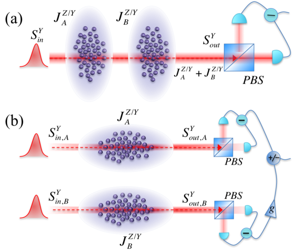
The experiments [60, 61] detect entanglement using a “verifying pulse” that propagates through the two ensembles (Fig. 1a). The Stokes observable of the transmitted pulse is measured via the polarizing beam splitter. Using equations (6), the outcome for the Stokes observable allows the value of the collective spin to be inferred. The measurement of proceeds similarly, after rotation of the atomic spin. The measurement scheme thus establishes the collective spin by a final projective measurement at one location. The quality of the measurement improves as becomes larger.
For smaller , the noise levels of the output become dominated by the vacuum noise of the input pulse. In that case, quantum noise squeezing of the input Stokes observable would improve the signal to noise ratio of the measurement.
3.1 Modification of the measurement strategy
To carry out an EPR experiment, it is necessary to make local measurements of and individually, and to then obtain the collective spin sum by addition of the measurement outcomes. Similarly, one should measure in a separate experimental procedure.
In order to achieve these goals, one possible strategy is to use two verifying pulses, defined with Stokes parameters and , propagating through each ensemble and respectively (as shown in Fig. 1b). The outputs in terms of the inputs are given by the solutions Eq. (5), so that
| (10) |
Measurement of at one location, and at the other location, enables local determination of and , as required for a test of EPR nonlocality. The local measurements of and can be made similarly. The quality of the measurement of the atomic spins improves when is large, or if the input fields are “squeezed”, so that and .
4 Detailed calculation for an engineered dissipative system
The recent experiment of Krauter et al [61] employs an engineered dissipative process to generate a long-lived entanglement between the atomic ensembles. The engineered dissipation approach offers a means to tailor dissipative processes, to enhance the generation of entangled or EPR states [45, 73]. Entanglement values of were achieved, using this process, in reasonable agreement with the theory presented by Muschik, Polzik and Cirac (MPC) [63, 62] for this experiment. We therefore analyse that theory, to calculate whether the EPR paradox is predicted for a complete and realistic atomic model.
The MPC model introduces operators , , where denote collective spin operators with and such that and , and . Here, the two-level states given in the definitions for the spins of ensemble / refer only to the ensemble / respectively. The and characterize a squeezed state with squeeze parameter , where and . The and are functions of the Zeeman splitting of the two atomic energy levels and of the detuning of the laser that couples these levels to the excited states and to vaccum modes, as detailed in Ref. [63]. The work of Muschik et al [63] shows how the correlations are described by a master equation [61]
| (11) | |||||
where is the atomic density operator, is the optical depth of an ensemble and is the single atom radiative decay. The represent the detrimental processes such as single atom spontaneous emission noise, thermal effects and collisions which counter the development of the entangled state, but which are included in the analysis to give a realsitic prediction. The Lindblad terms given in the parentheses arise from the engineered dissipative mechanism that drives the system into the EPR state [61]. For large optical depth , these entangling effects are enhanced. Other parameters are the number of atoms and in each of the two levels; and the normalized population where is the number of atoms in the two-level system.
4.1 Correlation dynamics
MPC derive the following dynamical equations for the evolution of the atomic spin correlations:
| (12) | |||||
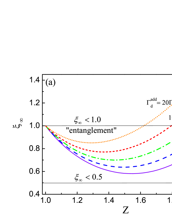
where , is the total single-particle cooling (heating) rate and is the total dephasing rate. The entangling terms of Eq. (11) arise as those being proportional to and will drive the system into an entangled EPR state. From this set of equations, in order to evaluate the predictions for the entanglement parameter , MPC derive an equation describing the evolution of the variances . The results of solving these equations in the steady-state are given in Fig (2), in the first panel, which plots the steady-state entanglement . This is clearly adequate for demonstrating entanglement, since variance sums of this type are an entanglement witness, as explained in the previous sections. These types of correlations were measured in the original experiment, as illustrated in Fig (1).
However, as we explain in greater detail below, these variance sums are not sufficient to demonstrate the stronger EPR requirement that we are interested in here. In fact, variance sums can be used as an EPR witness, provided correlations are strong enough and causality requirements are satisfied. The problem is that under the conditions of these experiments, with relatively imperfect correlations, variance sums are not an efficient witness. In simple terms, the use of this type of witness does not lead to evidence for an EPR paradox. The observed correlation strength in these experiments is not strong enough.
For the purpose of this paper, it is better, instead, to directly investigate the conditional variances which are at the heart of the inferred Heisenberg inequality.
4.2 Conditional variance calculation
To obtain the optimal prediction for the EPR paradox we need to modify the MPC analysis, to calculate the evolution of the conditional variances, and , as given by Eq. (4). These EPR variances can be measured by the arrangement of Fig. 1b. The equations are
The steady state solutions are given by
where and , and we have chosen the gains such that:
| (13) |
to minimize the conditional EPR variances. The steady state solution for is given by Muschik et al [63], as
| (14) |
These inferred variances correspond to quantities that would be measurable in the second type of experiment illustrated in Fig (1). So far, this type of experiment with local measurements at each site has not been carried out. The important issue is to be able to measure the spin of each atomic ensemble individually, in order to calculate the inferred or conditional variance.
4.3 EPR paradox predictions
We can define from the EPR paradox condition (3) the normalized EPR paradox parameter
| (15) |
that gives an indication of the amount of EPR paradox. The EPR paradox is obtained when and is strongest as [9]. We note the asymmetry of this definition, with relation to the subsystems and .
An EPR paradox is also obtained when . Either condition ( or ) is sufficient to demonstrate the paradox, and for asymmetric systems, where the parameters are not equal, this fact can become important and interesting [74, 76, 77, 75]. Recent work identifies as a criterion to verify an “EPR steering” of Alice’s system , by Bob’s measurements on system [17, 18, 19]. The asymmetry of definition is inherent in the original argument of EPR.
The steady state solution for the EPR parameter is given as
| (16) |
and is plotted in the Figure 2. Entanglement is verified if where
| (17) |
and we introduce the notation to remind us that there is a dependence on the experimental parameters and [78, 79, 80]. This criterion is more general than the symmetric criterion (7) of Duan et al [69]. We note that when . We introduce the notation used by Muschik et al: is the value of in the steady state, and is the steady state value of .
An important point is that the choice for and to minimize is not the same choice that will minimize the entanglement parameter . In fact, for ensembles symmetric under interchange , it is possible to show that is minimized by . In this case, . The steady state value of the entanglement parameter denoted is plotted in Fig. 2a, in agreement with Muschik et al [63]. As explained in Section 3, the observation of would imply the correlations of an EPR paradox. However, we see from the Fig. 2a that this cannot be achieved, for the parameter range chosen.
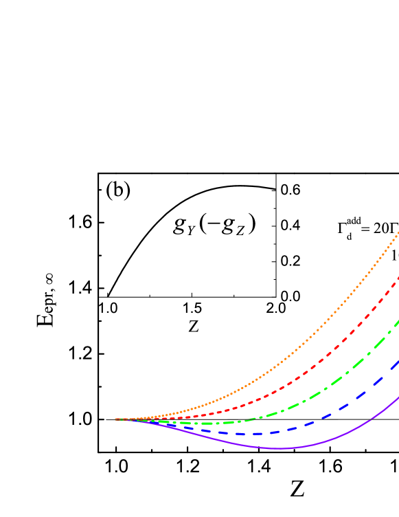
We plot the prediction for the EPR paradox in Fig. 2b, using the optimal arrangement of Fig 1b, where the gain factors and are selected as in (13) different to . We use the same parameters as for Figure 2a, that are selected by Muschik et al [63] to model the ensembles realistically in the experimental regime. Values of are predicted for mainly pure radiative damping. In the same regime, values of for the steady state entanglement are predicted. The EPR paradox parameter is more sensitive to dephasing than is entanglement. Given that the experiment has achieved a steady state entanglement of however, a realisation of an EPR paradox would seem feasible.
5 Discussion
The evidence for quantum nonlocality becomes compelling if the entangled systems are separated to the extent that the measurements made on the atomic ensembles by the verifying pulses are space-like separated events [24]. This consolidates the locality premise because then one can rule out a causal influence on the system due to measurements at . The measurement events are made in the time taken for the verifying pulse to interact with the individual ensemble. We denote this time as . Based on the description of the experiment of Ref. [60, 61], for that case, ms.
The entangling pulse (or engineered entanglement mechanism, as discussed above) must in the first instance be able to propagate through both ensembles to create the entanglement. It is also necessary that the entanglement lifetime exceed the measurement time, a condition that is clearly satisfied for the experiments of [61] which report entanglement times of up to s.
The separation between the ensembles must then be at least , which gives a requirement of much larger than room size separations found in current experiments. We therefore propose that the Polzik-type set-up, which is spatially separated but not strictly causal, would be a first step in which one obtains correlations of enough strength to guarantee the EPR paradox. A necessary subsequent experiment using pulsed entanglement with causal separation would be needed for a full EPR paradox demonstration. We note that pulsed local oscillator measurements provide well-defined properties analogous to the quadrature variables defined here [81]. Such quadrature measurements have been carried out previously for purely optical systems [82]. They are not impossible in a future, fully causal experiment on correlated atomic ensembles.
A second potential criticism of the proposed experiment is the nature by which the macroscopic atomic spin of the atomic ensembles are measured. The value for the spin is inferred via the relationship given by equations (10), based on the measurement of the Stokes field observables. The validity of the measurement then depends on the correctness of the quantum based equations, which involves the question of Gaussian mode-coupling constants [83] and the corresponding noise calibration issues. In this respect, the proposals such as given in Ref. [29, 40] to realize an EPR paradox based on the spin observables of two groups of atoms of a Bose Einstein Condensate (BEC), by using four-wave mixing or molecular dissociation, provide an important alternative. Here, each group of atoms can be constrained spatially by the potential well of an optical lattice. While the spatial separations are therefore limited, the advantage is that atomic populations are measured directly by atomic imaging, which simplifies calibration issues. Other advantages that exist include the possibility of longer decoherence times [84] and reduced atomic dephasing which the theory summarized in Section IV indicates is detrimental to the EPR correlations.
Perhaps the most fascinating feature of the current proposal is the macroscopic nature of the EPR correlations. The EPR observables are the Schwinger atomic spins, which correspond to the difference in the numbers of atoms populating two specified atomic states. For these experiments, the total atom numbers are large ( atoms). The atom number differences do not need to be measured microscopically that is, with a microscopic precision where single atoms are distinguished in order to attain the EPR paradox. The reason for this is understood by examining the EPR paradox condition (3), and noticing that the right side depends on the total mean spin which is given as [85]. The quantum noise level of the uncertainty relation becomes a macroscopically measurable quantity, thus enabling the paradox to be realized based on the ratio (15) only.
6 Conclusion
In summary, we have examined the possibility of detecting an EPR paradox between two macroscopic atomic ensembles at room temperature, based on the experiments that have realized an entanglement between the ensembles. Although the realisation of an EPR paradox is more difficult than for entanglement, detailed models that account for decoherence effects allow prediction of the EPR paradox, for room temperature atoms. We have shown that the measurement scheme must be modified, to enable local measurements on each ensemble to be performed. The proposed experiment would be a convincing demonstration of quantum nonlocality in the form of the EPR paradox and quantum steering for truly macroscopic objects.
References
- [1] Einstein A, Podolsky B and Rosen N 1935 Phys. Rev. 47 777
- [2] Wu C S and Shaknov I 1950 Phys. Rev. 77 136
- [3] Bell J S 1964 Physics 1 195
- [4] Clauser J F et al 1969 Phys. Rev. Lett. 23 880
- [5] Aspect A, Grangier P and Roger G 1982 Phys. Rev. Lett. 49 91
- [6] Ou Z Y et al 1992 Phys. Rev. Lett. 68 3663
- [7] Aspect A, Dalibard J and Roger G 1982 Phys. Rev. Lett. 49 1804; Kwiat P G et al 1995 Phys. Rev. Lett. 75 4337; Weihs G et al 1998 ibid. 81 5039; Tittel W et al 2000 ibid. 84 4737
- [8] Reid M D 1989 Phys. Rev. A 40 913
- [9] Reid M D et al 2009 Rev. Mod. Phys. 81 1727 and experiments referenced therein
- [10] Howell J C et al 2004 Phys. Rev. Lett. 92 210403
- [11] Wang Y et al 2010 Opt. Express 18(6) 6149
- [12] Hage B, Samblowski A and Schnabel R 2010 Phys. Rev. A 81 062301; Eberle T et al 2011 Phys. Rev. A 83 052329; Takei N et al 2006 Phys. Rev. A 74 060101(R); Samblowski A et al 2011 AIP Conf. Proc. 1363 219; Steinlechner S et al 2013 Phys. Rev. A 87 022104
- [13] Boyer V et al 2008 Science 321 544
- [14] Wagner K et al 2008 Science 321 541
- [15] Ch. Silberhorn et al 2001 Phys. Rev. Lett. 86 4267; Zhang Y et al 2000 Phys. Rev. A 62 023813
- [16] Bowen W P et al 2002 Phys. Rev. Lett. 89 253601
- [17] Wiseman H M, Jones S J and Doherty A C 2007 Phys. Rev. Lett. 98 140402
- [18] Jones S J, Wiseman H M and Doherty A C 2007 Phys. Rev. A 76 052116
- [19] Cavalcanti E G et al 2009 Phys. Rev. A 80 032112
- [20] Schrödinger E 1935 Proc. Cambridge Philos. Soc. 31 553; 1936 ibid. 32 446
- [21] Saunders D J et al 2010 Nat. Phys. 6, 845
- [22] Smith D H et al 2012 Nature Commun. 3 625
- [23] Bennet A J et al 2012 Phys. Rev. X 2 031003
- [24] Wittmann B et al 2012 New J. Phys. 14 053030
- [25] Liebfried D et al 2005 Nature 438 639
- [26] Monz T et al 2011 Phys. Rev. Lett. 106, 130506
- [27] Rowe M A et al 2001 Nature 409 791
- [28] Ansmann M et al 2009 Nature 461 504
- [29] Gross C et al 2011 Nature 480 219
- [30] Esteve J et al 2008 Nature 455 1216
- [31] Bücker R et al 2011 Nature Phys. 7 608
- [32] Bücker R et al 2012 Phys. Rev. A 86 013638
- [33] Erdosi D et al 2013 New J. Phys. 15 023033
- [34] Chaneliere T et al 2005 Nature 438 833
- [35] Choi K S et al 2008 Nature 452 67
- [36] Josse V et al 2004 Phys. Rev. Lett. 92 123601
- [37] Matsukevich D N and Kuzmich A 2004 Science 306 663
- [38] Chou C W et al 2005 Nature 438 828
- [39] Shi Y 2001 Int. J. Mod. Phys. B 15 3007; Shi Y and Niu Q 2006 Phys. Rev. Lett. 96 140401; Shi Y 2010 Phys. Rev. A 82 023603
- [40] Opatrny T and Kurizki G 2001 Phys. Rev. Lett. 86 3180; Barut A O and Meystre P 1984 Phys. Rev. Lett. 53 1021; Kheruntsyan K V, Olsen M K and Drummond P D 2005 Phys. Rev. Lett. 95 150405
- [41] Ferris A J et al 2008 Phys. Rev. A 78 060104(R)
- [42] Bar-Gill N et al 2011 Phys. Rev. Lett. 106 120404
- [43] He Q Y et al 2011 Phys. Rev. Lett. 106 120405
- [44] He Q Y et al 2012 Phys. Rev. A 86 023626
- [45] Opanchuk B et al 2012 Phys. Rev. A 86 023625
- [46] Lewis-Swan R J and Kheruntsyan K V arXiv:1304.0297 [quant-ph]
- [47] Gabriel A and Hiesmayr B C 2013 Euro. Phys. Lett. 101 30002
- [48] Vedral V, 2008 Nature 453 1004
- [49] Furry W H 1936 Phys. Rev. 49 393
- [50] Bertlmann R A, Grimus W and Hiesmayr B C 1999 Phys. Rev. D 60 114032; Peres A and Singer P 1960 Il Nuovo Cimento, 15, 907
- [51] Schrödinger E 1935 Naturwissenschaften 23 844
- [52] Leggett A J, 2002 J. Phys. Condens. Matter 14 R415
- [53] Ralph T C 1999 Phys. Rev. A 61 010303(R)
- [54] Reid M D 2000 Phys. Rev. A 62, 062308
- [55] Silberhorn Ch et al 2002 Phys. Rev. Lett. 88, 167902
- [56] Grosshans F et al 2003 Nature 421, 238
- [57] Grosshans F and Grangier P 2001 Phys. Rev. A 64, 010301
- [58] Branciard C et al 2012 Phys. Rev. A 85, 010301(R)
- [59] Berta M et al 2010 Nature Physics 6 659
- [60] Julsgaard B, Kozhekin A and Polzik E S 2011 Nature 413 400
- [61] Krauter H et al 2011 Phys. Rev. Lett. 107 080503
- [62] Muschik C A et al 2012 J. Phys. B: At. Mol. Opt. Phys. 45 124021
- [63] Muschik C A, Polzik E S and Cirac J I 2011 Phys. Rev. A 83 052312
- [64] Lee K C et al 2011 Science 334 1253
- [65] Duan L M, Cirac J, Zoller P and Polzik E 2000 Phys. Rev. Lett. 85 5643
- [66] Cavalcanti E G and Reid M D 2007 Journ. Mod. Opt. 54 2373
- [67] Cavalcanti E G et al 2009 Optics Express 17 18693
- [68] Walborn S et al 2011 Phys. Rev. Lett. 106, 130402
- [69] Duan L M et al 2000 Phys. Rev. Lett. 84 2722
- [70] Raymer M et al 2003 Phys. Rev. A 67 052104
- [71] Sorensen A S and Molmer K 2001 Phys. Rev. Lett. 86 4431
- [72] He Q Y et al 2011 Phys. Rev. A 84 022107
- [73] Mogilevtsev D et al quant-ph arXiv: 1211.4435
- [74] Midgley S L W, Ferris A J and Olsen M K 2010 Phys. Rev. A 81 022101
- [75] Wagner K et al arXiv:1203.1980 [quant-ph]
- [76] Händchen V et al 2012 Nature Photonics 6 598
- [77] Cavalcanti E G et al 2011 Phys. Rev. A 84 032115
- [78] Braunstein S et al 2001 Phys. Rev. A 64 022321
- [79] Giovannetti V et al 2003 Phys. Rev. A 67 022320
- [80] Mancini S et al 2002 Phys. Rev. Lett. 88 120401
- [81] Drummond P D 1990 Quantum Optics 2 205
- [82] Slusher R E et al 1987 Phys. Rev. Lett. 59 2566
- [83] Rosenberger A T et al 1991 Phys. Rev. A 43 6284
- [84] Egorov M et al 2011 Phys. Rev. A 84 021605
- [85] Reid M 2000 Phys Rev. Lett. 84 2765