Magnetic Reconnection under Anisotropic MHD Approximation

Abstract

We study the formation of slow-mode shocks in collisionless magnetic reconnection by using one- and two-dimensional collisionless MHD codes based on the double adiabatic approximation and the Landau closure model. We bridge the gap between the Petschek-type MHD reconnection model accompanied by a pair of slow shocks and the observational evidence of the rare occasion of in-situ slow shock observations. Our results showed that once magnetic reconnection takes place, a firehose-sense ($p_{||}>p_{\perp}$) pressure anisotropy arises in the downstream region, and the generated slow shocks are quite weak comparing with those in an isotropic MHD. In spite of the weakness of the shocks, however, the resultant reconnection rate is $10-30\%$ higher than that in an isotropic case. This result implies that the slow shock does not necessarily play an important role in the energy conversion in the reconnection system, and is consistent with the satellite observation in the Earth’s magnetosphere.

I Introduction

Magnetic reconnection has been widely studied as an efficient mechanism for converting magnetically stored energy to thermal and/or kinetic energy in plasmas. It appears in various phenomena in astrophysics and space physics, e.g., the magnetopause where the Earth’s magnetic field reconnects with the interplanetary magnetic field carried by the solar wind, Sckopke1981 ; Hesse1994 ; Frey2003 the magnetotail where the field lines stretched by the solar wind reconnect with each other, Oieroset2001 ; Nagai2001 ; Zenitani2012 and solar flares where enormous energy and mass are released by magnetic reconnection.Parker1963 ; Kopp1976 ; Masuda1994 The common feature of these plasmas is that the magnetic Reynolds numbers are extremely large and classical Ohmic dissipation cannot explain the rates of energy release.Sweet1958 ; Parker1957 To overcome this problem, Petschek pointed out that the reconnection accompanied by a pair of slow shocks emanating from the X-type diffusion region could provide a fast reconnection rate even in plasmas with high Reynolds numbers.Petschek1964

In fact, numerous researchers have demonstrated the fast reconnection with a pair of slow shocks in MHD nonlinear simulations. However, it is rare for the formation of the Petschek-type slow shock to be detected in current sheets by in-situ observations.Saito1995 ; Seon1996 Furthermore, the recent advances in computational power have enabled particle-in-cell and hybrid simulations of collisionless plasmas, Liu2011a ; Higashimori2012 ; Weng2012 ; Hoshino1998 but the results do not provide clear evidence for the formation of the slow shock. It is thought that the absence of shocks in kinetic simulations might be caused by the smallness of the simulation box or by the pressure anisotropy due to the PSBL (plasma sheet boundary layer) ion beams accelerated along the magnetic field lines from the diffusion region. Higashimori2012 ; Liu2011a In fact, a large pressure anisotropy with $p_{||}>p_{\perp}$ has been observed during reconnection in the magnetotailHoshino2000 .

In this paper, in order to bridge the gap between the Petschek model with its slow-mode shocks and the kinetic simulation results and observations, we perform a series of collisionless MHD simulations, paying special attention to the effect of a pressure anisotropy on the global dynamics of a reconnection layer. We use the MHD equations combined with an anisotropic pressure tensor, the double adiabatic approximation, and the Landau closure model as a basis for collisionless fluid formulation.

The outline of this paper is as follows. In Section II, we briefly introduce the basic equations for collisionless MHD and explain the setups of our simulations. Section III shows the results of one- and two-dimensional simulations, i.e., the 1-D result in Section III.1 and the 2-D result in Section III.2. The concluding Section IV includes the summary and implications of the results of this paper.

II Basic Equations and Simulation Models

II.1 Collisionless MHD Equations

In the MHD limit in which all scales of fluctuations are much larger than the ion Larmor radius and all frequencies are much lower than the ion cyclotron frequency, the governing equations of a collisionless plasma can be described by the Kulsrud’s formulation.Kulsrud1983 The basic equations we adopted are as follows:

$$\frac{\partial\rho}{\partial t}+{\bm{\nabla}}\cdot\left(\rho{\bm{V}}\right)=0,$$ (1)

$$\frac{\partial}{\partial t}\left(\rho{\bm{V}}\right)+{\bm{\nabla}}\cdot\left[\rho{\bm{V}}{\bm{V}}+\left({\bm{P}}+\frac{B^{2}}{8\pi}{\bm{I}}\right)-\frac{{\bm{B}}{\bm{B}}}{4\pi}\right]=0,$$ (2)

$$\frac{\partial{\bm{B}}}{\partial t}={\bm{\nabla}}\times\left({\bm{V}}\times{\bm{B}}\right)-{\bm{\nabla}}\times\left(\eta{\bm{\nabla}}\times{\bm{B}}\right),$$ (3)

$${\bm{P}}=p_{\perp}{\bm{I}}+\left(p_{||}-p_{\perp}\right){\hat{\bm{b}}}{\hat{\bm{b}}},$$ (4)

where $\rho$ is the mass density, ${\bm{V}}$ is the balk velocity, ${\bm{B}}$ is the magnetic field vector, ${\bm{I}}$ is the unit tensor, $\eta$ is the magnetic diffusivity, $\hat{\bm{b}}={\bm{B}}/B$ is the unit vector parallel to the magnetic field, and ${\bm{P}}$ is the pressure tensor with the different components $p_{\perp}$ and $p_{||}$, which are respectively perpendicular and parallel to the background magnetic field.

Equations of state for determination of $p_{\perp}$ and $p_{||}$ are given below. Taking the second moments of a drift kinetic equation leads to a set of equations of state as followsChew1956 :

$$\rho B\frac{D}{Dt}\left(\frac{p_{\perp}}{\rho B}\right)=-{\bm{\nabla}}\cdot{\bm{q}}_{\perp}-q_{\perp}{\bm{\nabla}}\cdot{\hat{\bm{b}}},$$ (5)

$$\frac{\rho^{3}}{B^{2}}\frac{D}{Dt}\left(\frac{p_{||}B^{2}}{\rho^{3}}\right)=-{\bm{\nabla}}\cdot{\bm{q}}_{||}+2q_{\perp}{\bm{\nabla}}\cdot{\hat{\bm{b}}},$$ (6)

where ${\bm{q}}_{\perp,||}=q_{\perp,||}{\hat{\bm{b}}}$ are the heat fluxes along the magnetic field and $D/Dt=\partial/\partial t+{\bm{V}}\cdot{\bm{\nabla}}$ is the fluid Lagrangian derivative. It can be seen from eqs. (5) and (6) that if the effects of heat fluxes are neglected (the so-called double adiabatic limit or the CGL approximation), the quantities enclosed in parentheses on the left-hand sides are conserved and then $p_{\perp}\propto\rho B$ and $p_{||}\propto\rho^{3}B^{-2}$. When considering magnetic reconnection, it appears, therefore, that the reduction of magnetic field strength and the increase of plasma density across the plasma sheet boundary naturally leads to pressure anisotropy with $p_{||}>p_{\perp}$.

For a model of the heat flux, we employed the Landau closure model, Hammett1990 ; Hammett1992 ; Snyder1997 which can correctly describe the kinetic linear Landau damping process. The functional forms of the linearized heat flux in Fourier space can be written as

$${\tilde{q}}_{||}=-\sqrt{\frac{8}{\pi}}\rho_{0}c_{||0}\frac{ik_{||}\left(p_{||}/\rho\right)}{\left|k_{||}\right|},$$ (7)

$${\tilde{q}}_{\perp} = -\sqrt{\frac{2}{\pi}}\rho_{0}c_{||0}\frac{ik_{||}\left(p_{\perp}/\rho\right)}{\left|k_{||}\right|}$$ (8)

$$+\sqrt{\frac{2}{\pi}}c_{||0}\frac{p_{\perp 0}}{B_{0}}\left(1-\frac{p_{\perp 0}}{p_{||0}}\right)\frac{ik_{||}B}{\left|k_{||}\right|},$$

where subscript $0$ denotes the equilibrium values, $c_{||0}=\left(p_{||0}/\rho_{0}\right)^{1/2}$ is the parallel thermal velocity, and $k_{||}$ is the parallel wavenumber. The first terms in both eqs. (7) and (8) represent the effect of heat conduction, and the second term in eq. (8) shows the flux due to the magnetic field gradient, which is important for correctly reproducing the threshold of mirror instabilities.

Real space expressions of these closure equations are given by convolution integrals along the magnetic field line. In this paper, to avoid the expensive routine of performing Fourier transformation along tangled field lines, we follow the same procedure by Sharma et al.Sharma2006 We pick out one characteristic wavenumber $k_{L}$ along the field line which represents the length scale of collisionless linear Landau damping and adopt the local approximation in Fourier space. Hence $ik_{||}$ and $|k_{||}|$ in eqs. (7) and (8) are replaced by $\nabla_{||}={\hat{\bm{b}}}\cdot{\bm{\nabla}}$ and $k_{L}$, respectively.

Since a finite electric conductivity is assumed for this reconnection study, Ohmic heating terms should be added explicitly in the right-hand sides of eqs. (5) and (6). In the anisotropic MHD, however, the ratio of energy distribution to parallel and perpendicular thermal energy cannot be self-consistently determined. Here we assume that Ohmic heating is mainly caused by electrons rather than ions, and that the colliding electrons with waves are rapidly isotropized. Hence the same amount of energy is deposited into each degree of freedom by

$$\frac{d}{dt}\left(\frac{p_{||}}{\gamma_{||}-1}\right)_{\rm Ohm}\!\!\!=\frac{f_{||}}{f_{||}+f_{\perp}}\eta J^{2},$$ (9)

$$\frac{d}{dt}\left(\frac{p_{\perp}}{\gamma_{\perp}-1}\right)_{\rm Ohm}\!\!\!=\frac{f_{\perp}}{f_{||}+f_{\perp}}\eta J^{2},$$ (10)

where $f_{||}=1$ and $f_{\perp}=2$ are the degree of freedom parallel and perpendicular to the local magnetic field lines, respectively. $\gamma_{||,\perp}=(f_{||,\perp}+2)/f_{||,\perp}$ are adiabatic indices.

II.2 Simulation Setup

In our simulation study, we solve the continuity equation (1), the momentum conservation equation (2), the induction equation (3), the equations of state (5) and (6) combined with Ohmic heating terms (9) and (10), and the heat flux (7) and (8) under the Fourier-space local approximation.

As an initial state, we assume a static, isothermal, and isotropic plasma with the Harris-type current sheet:

$$B_{X}=B_{X0}\tanh(Z/L),$$ (11)

$$p_{||}=p_{\perp}=p_{0}+\frac{B_{X0}^{2}}{8\pi}\cosh^{-2}(Z/L).$$ (12)

The subscript 0 denotes the lobe region, and the plasma beta in the lobe region is set at $0.25$. Since the magnetic field strength appears in the denominator when determining the direction of the magnetic field and calculating the heat flux, we discuss the guide-field reconnection with a finite uniform guide field component $B_{Y}$ so as to avoid zero division near the neutral sheet. The strength of the guide field is characterized by $\phi$, which is the angle between the tangential magnetic field and the X-axis, i.e., $\tan\phi=B_{Y}/B_{X0}$. $\phi=0^{\circ}$ corresponds to a purely anti-parallel case, and the $\phi=90^{\circ}$ case has no anti-parallel component.

The spatial scale is normalized by the half thickness of the current sheet, $L$, and the velocity is normalized by the ${\rm Alfv\acute{e}n}$ velocity defined in the lobe region far from the X-point, $V_{A}$. The time scale is normalized by the ${\rm Alfv\acute{e}n}$ transit time, $L/V_{A}$. The magnetic pressure and gas pressure are normalized by twice the lobe magnetic pressure, $\left(B_{X0}^{2}+B_{Y0}^{2}\right)/4\pi$. The background magnetic Reynolds number is set to $Re=500$ and the anomalous resistivity with $Re=80$ is assumed at the origin. We solved the region $X=0,\ -200<Z<200$ with $4000$ grid points in 1-D simulations and $0<X<500,\ -50<Z<50$ with $5000\times 1000$ grid points in 2-D simulations. In 1-D simulations, we set the normal component of the magnetic field $B_{Z}$ to $5\%$ of the total magnetic field in the lobe region. We imposed the symmetric boundary condition on $X=0$ and the free boundary conditions on other boundaries.

The basic equations are all discretized in space and time. Spatial derivatives are calculated by the 4th-order central differences, and temporal derivatives are integrated by the 4th-order Runge-Kutta scheme. A numerical error of ${\bm{\nabla}}\cdot{\bm{B}}$ is removed with the method used in Rempel et al.Rempel2009 Furthermore, for the purpose of capturing shock waves, an artificial diffusivity is imposed upon all MHD variables at every time step. Rempel2009

III Collisionless MHD Simulation Results

III.1 1-D Riemann Problem

If the steady-state reconnection can be realized in two-dimensional space, we may discuss the structure of reconnection as a solution of the one-dimensional Riemann problemTsai2006 ; Heyn1988 . Before proceeding to the 2-D results, we shall look at the qualitative characteristics of reconnection layers in the anisotropic MHD. The heat flux is set to zero in this subsection in order to clearly observe a discontinuity. We note that the presence of the heat flux does not change the fundamental reconnection structure.

Shown in Fig. 1 are the results with $\phi=30^{\circ}$, the isotropic MHD case Fig. 1(a) and the MHD+CGL case Fig. 1(b). The most striking difference between the isotropic and anisotropic cases is the sequence of propagation of slow-mode waves and ${\rm Alfv\acute{e}n}$ waves or rotational waves, which can be seen clearly by comparing the velocity profiles. As we have expected, the parallel pressure is more highly enhanced across the slow shock than the perpendicular pressure in the CGL case. From the next subsection, we discuss the isotropic and anisotropic results one by one in order to clearly understand the differences.

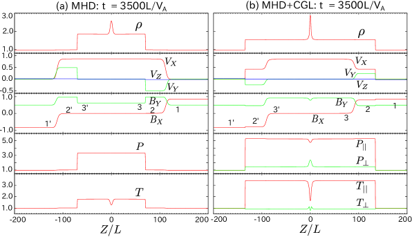
Figure 1: The spatial distribution of variables at time $t=3500L/V_{A}$ with $\phi=30^{\circ}$. (a)MHD, and (b)MHD+CGL.

First, we shall discuss the results in the isotropic MHD case. In all calculations, first of all, a pair of the fast rarefaction waves propagate away from the simulation domain by the time about $t=200-300L/V_{A}$. If the lobe magnetic field lines are completely anti-parallel, a pair of switch-off slow shocks should propagate outward from the neutral point. In the case of the guide field reconnection, however, we can clearly see the propagation of the rotational discontinuities ahead of the slow shocks, which are regarded as finite amplitude ${\rm Alfv\acute{e}n}$ waves. Since the initial magnetic field configuration violates the coplanarity, and since the slow shocks alone cannot connect both lobe regions consistently, the rotational waves are generated so as to maintain the coplanarity downstream.

Behind the rotational discontinuity, we can find the slow shock, where the density, the pressure, and the temperature increase. We find that the compression ratio of density is 1.88 across the shock.

A hodogram is useful to understand the behavior of the discontinuities. Fig. 2(a) shows the magnetic field in the isotropic MHD case with $\phi=10^{\circ},30^{\circ},50^{\circ},$ and $70^{\circ}$. In order to focus on the shock structure, the data in the region of $|Z|<10L$, where the effect of the initial current sheet remains, are removed in the hodograms. Numbers in the panel for $\phi=30^{\circ}$ indicate the spatial correspondence with Fig. 1. When crossing the rotational discontinuity, the trajectory draws a circle with the center at the origin (1-2,1’-2’), which means the magnetic field changes its direction with the magnetic field energy conserved. When a slow shock passes, on the other hand, the distance from the origin in the hodogram decreases (2-3,2’-3’), which corresponds to the reduction of the magnetic energy. In Fig. 2(a), these reductions appear as vertical trajectories along the $B_{Y}$ axis. As the shear angle $\phi$ increases, the vertical displacement becomes small (i.e., decrease in released magnetic energy), but the topological structure of a reconnection layer does not change.Tsai2006

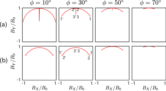
Figure 2: The hodograms of magnetic fields at time $t=3500L/V_{A}$. (a)MHD case, and (b)MHD+CGL case.

Next, we shall look at the anisotropic case of Fig. 1(b). After a pair of fast rarefaction waves propagate away by the time about $t=200-250L/V_{A}$, the slow shocks appear ahead of the rotational discontinuities. All physical quantities sharply change when crossing the slow shock as in the isotropic case. Although both parallel and perpendicular pressures increase across the shock, the parallel pressure is preferentially enhanced. It is notable that the temperature calculated from the perpendicular pressure slightly decreases, which implies that the required entropy increase across the shock is predominantly provided in the parallel direction. The anisotropy parameter, $\varepsilon=1-4\pi\left(p_{||}-p_{\perp}\right)/B^{2}$, is about 0.43 in this $\phi=30^{\circ}$ case.

The compression ratio of plasma density from the lobe to the inner plasma sheet becomes 1.58, which is less than that in the isotropic MHD case by about 16%. The shear angle dependence of the compression ratio is summarized in Fig. 3. The plus and cross symbols indicate the MHD and MHD+CGL cases, respectively. They are fitted by $a\cos^{2}\phi+1$ curves. The top panel shows the ratio of compression ratio in anisotropic calculations to that in the isotropic ones, and the solid line indicates the ratio obtained by the $a\cos^{2}\phi+1$ curve fit in the bottom panel. A common feature in a wide range of shear angles is that the compression ratio decreases in an anisotropic MHD. In other words, the slow shock in the anisotropic MHD is always weaker than that in the isotropic MHD. The ratio weakly depends on the shear angle, but it has a value from 0.8 to 1.0.

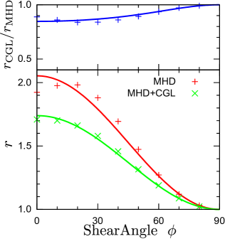
Figure 3: Shear angle dependence of the compression ratio of plasma density across the slow shocks. In the bottom panel, two types of points indicate $r=\rho_{\rm down}/\rho_{\rm up}$ measured in 1-D simulations of isotropic and anisotropic MHD. Solid lines are fitting functions with the form of $a\cos^{2}\phi+1$. The top panel shows the ratio of $r$ in the anisotropic MHD to that in the isotropic MHD.

The most striking modification from the isotropic case is that the slow shocks are formed ahead of the rotational waves. It is known that under the presence of the pressure anisotropy, the phase speed of an ${\rm Alfv\acute{e}n}$ wave is reduced to the value $V_{A}^{*}=\sqrt{\varepsilon}V_{A}$. The phase speed of slow modes, on the other hand, increases for an oblique propagation to the background magnetic field. Such a correction of each phase velocity modifies the structure of the reconnection layer. The antecedent of slow shocks can also be verified in the hodogram in Fig. 2(b). The reduction of the magnetic field (1-2, 1’-2’) occurs before the rotational waves (2-3, 2’-3’). The same behavior can be seen in the case of $\phi=10^{\circ}$. In the two panels of $\phi=50^{\circ}$ and $\phi=70^{\circ}$ on the right, on the other hand, the rotation appears in the lobe side.

The relation between the shear angle $\phi$ and the positions of wave-fronts are summarized in Fig. 4, for (a)MHD cases, and (b)MHD+CGL cases. Both the plus symbols and the red lines represent the front position of the ${\rm Alfv\acute{e}n}$ waves, while the cross symbol and green lines are the slow mode waves. The plus and cross symbols indicate respectively the positions at the peak parallel or perpendicular current density measured in our simulation. Since an ${\rm Alfv\acute{e}n}$ wave only rotates in the direction of the magnetic field, it can generate current only parallel to the field line. Hence, the location at the peak of the parallel current profile can be regarded as the ${\rm Alfv\acute{e}n}$ wave front, and the location where the perpendicular current becomes largest can be regarded as the slow-mode wave front. The solid lines represent the theoretical distance estimated by the product of the lapsed time and the phase velocity calculated from simulation data behind each wave front. The good agreement between the solid lines and dots confirms that the rotation and reduction of the magnetic field are indeed caused by ${\rm Alfv\acute{e}n}$ waves and slow-mode waves, respectively. In the anisotropic case, as the shear angle increases, the anisotropy parameter $\varepsilon$ arising downstream approaches the isotropic value, i.e., $\varepsilon\to 1$. Hence, as described above, the modified ${\rm Alfv\acute{e}n}$ velocity $V_{A}^{*}$ becomes larger as increasing the shear angle $\phi$ increases. The slow-mode velocity, on the other hand, decreases with $\phi$. As a result, rotational waves forego slow shocks for the shear angle greater than about $43^{\circ}$, while the rotational waves always form in front of the slow shocks in the isotropic MHD.

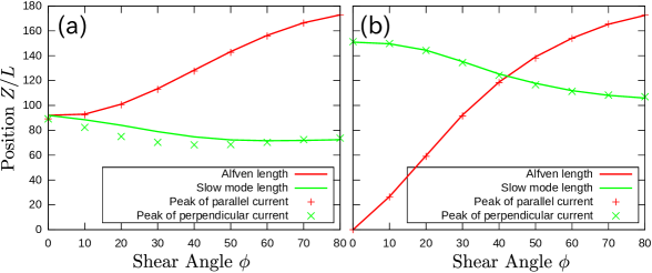
Figure 4: The relation between the shear angle $\phi$ and the wave-front of each mode. The positions at the peak parallel and perpendicular current density can be regarded as the ${\rm Alfv\acute{e}n}$ wave-front and the slow wave-fronts respectively. The solid lines are the theoretical propagation length obtained from simulation data. (a) shows MHD, and (b) MHD+CGL.

Next, we shall discuss the relation between the in-/out-flow velocities and the guide field. The dependence of outflow velocities upon the shear angle $\phi$ is quite different between isotropic and anisotropic cases, particularly for the cases when slow shocks precede rotational waves. The outflow speed in the 1-D simulation is shown in Fig. 5. The plus and cross symbols indicate respectively $V_{X}$ measured at $Z=0$ in the MHD and MHD+CGL calculations, and the solid curve shows the ${\rm Alfv\acute{e}n}$ velocity defined by an anti-parallel magnetic field component, i.e., $V_{A}\cos\theta$. The plus symbols of the isotropic MHD agree well with the ${\rm Alfv\acute{e}n}$ velocity measured by an anti-parallel magnetic field. For the anisotropic or MHD+CGL case, however, the outflow velocity becomes smaller than the ${\rm Alfv\acute{e}n}$ speed for $\phi\raisebox{-2.15277pt}{$\>\stackrel{{\scriptstyle\textstyle<}}{{\sim}}\>$}30^{\circ}$, at which slow shocks propagate faster than rotational waves. For a somewhat small $\phi$, the plasma flowing into a reconnection layer undergoes a two-step acceleration toward the $X$-direction, first by a slow shock, and then by a rotational wave. Since the released magnetic energy across a slow shock is very small in the anisotropic case, the resultant velocity across the shock becomes slower compared with the ${\rm Alfv\acute{e}n}$ velocity. For the case of $\phi\raisebox{-2.15277pt}{$\>\stackrel{{\scriptstyle\textstyle>}}{{\sim}}\>$}40^{\circ}$, a rotational wave propagates faster than a slow-mode wave, and then the final $V_{X}$ is determined only by the rotational discontinuity, and a slow shock just reduces $V_{Y}$. Thus, the sequence of wave propagation can control the nature of reconnection exhaust.

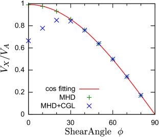
Figure 5: The dependence of outflow velocity upon the shear angle $\phi$. The plus and cross symbols indicate respectively $V_{X}$ measured at $Z=0$ in isotropic and anisotropic MHD, and the solid curve shows the ${\rm Alfv\acute{e}n}$ velocity by anti-parallel magnetic field component, i.e., $V_{A}\cos\theta$.

We next discuss the reconnection rate, $M_{A}=V_{\rm in}/V_{A}$, defined by the inflow velocity and an upstream ${\rm Alfv\acute{e}n}$ velocity measured at $Z/L=200$. The relation between the reconnection rates and the shear angle surveyed by using 1-D simulations is summarized in Fig. 6. The notation of the symbols and solid lines are all same as Fig. 3, but the fitting curves have the functional forms of $a\cos^{2}\phi$ now. For a wide range of shear angles, reconnection rate slightly rises in the MHD+CGL cases. The ratio of the reconnection rates has a value from 1.1 to 1.3.

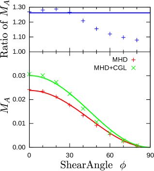
Figure 6: Shear angle dependence of inflow ${\rm Alfv\acute{e}n}$ Mach numbers, i.e., reconnection rates. In the bottom panel, two types of points indicate $V_{Z}/V_{A}$ measured at $Z/L=200$ in 1-D simulations of isotropic and anisotropic MHD. Solid lines are fitting functions proportional to $\cos^{2}\phi$. The top panel shows the ratio of reconnection rate in the anisotropic MHD to that in the isotropic MHD.

III.2 2-D Simulation with Guide Field

With the results of the 1-D simulation fully in mind, we shall now turn to the results of the 2-D simulations. Fig. 7 shows a typical case for a developed reconnection layer with the shear angle $\phi=30^{\circ}$ at time $t=600L/V_{A}$ for an anisotropic MHD calculation, i.e., a MHD + CGL + Landau Closure calculation. Each panel shows the color contours of $p_{||}$, $p_{\perp}$, $\varepsilon$, and $B^{2}$, normalized by the initial values in the lobe region respectively. Magnetic field lines are superposed by solid black lines. The results from an isotropic MHD calculation, the pressure and the magnetic energy, are shown in Fig. 8.

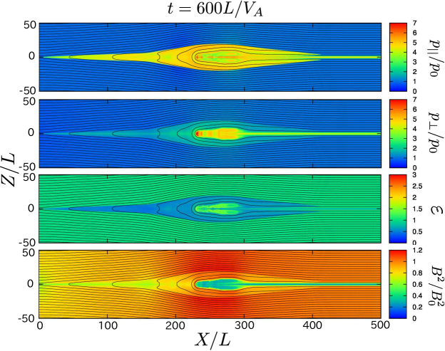
Figure 7: A snapshot of the MHD+CGL simulation with $\phi=30^{\circ}$ at time $t=600L/V_{A}$. Each panel shows the color contour of the parallel pressure, the perpendicular pressure, the anisotropy parameter, and the magnetic energy from top to bottom. All variables are normalized by the initial values in the lobe region. The solid lines indicate the magnetic field lines.

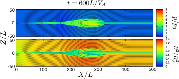
Figure 8: A snapshot of the isotropic MHD simulation with $\phi=30^{\circ}$ at time $t=600L/V_{A}$. The top and bottom panels show the color contours of the pressure and the magnetic energy, respectively, normalized by the initial values in the lobe region. The solid lines indicate the magnetic field lines.

Once magnetic reconnection occurs, a high pressure plasmoid consisting of the dense plasma that initially supports the plasma sheet is squeezed out to reconnection exhaust. In the post-plasmoid plasma sheet after the passage of the plasmoid, the parallel pressure in the outflow region is enhanced more intensively than the perpendicular pressure across a pair of the weak slow shock boundaries, as we have already seen in 1-D simulations. The magnetic energy is reduced in the reconnection layer, but the reduction occurs less sharply than that in the isotropic case (see the bottommost panels in Fig. 7 and Fig. 8). The downstream anisotropy parameter $\varepsilon\sim 0.45$ well agrees with the corresponding 1-D calculation. It is notable that the flaring angle sandwiched by two slow shocks becomes wider than the angle in an isotropic MHD simulation started from the same initial condition. For the shear angle $\phi=30^{\circ}$, these angles are $2.4^{\circ}$ in the MHD+CGL and $1.4^{\circ}$ in the MHD.

To illustrate the spatial distribution of the reconnection layer, a cross-sectional view of the current density along the $Z$-axis at $X=100L$ is shown in Fig. 9, (a) showing the isotropic MHD case, and (b) the anisotropic case. The top and bottom panels indicate the current density parallel and perpendicular to the background magnetic field, normalized by the initial field in the lobe region divided by the half width of the initial current sheet, $B_{0}/L$. The vertical lines indicate the locations where the current densities reach their maximum. Since $J_{||}$ and $J_{\perp}$ arise in rotational discontinuities and slow shocks respectively, as mentioned in the previous section, the vertical lines are marked by the scripts RD and SS. In fact, the rotational wave occupies a wider region here, and the slow shocks may be disguised. From the locations with the peak current density, however, it is clear that the slow shocks form in front of the rotational waves in the anisotropic case. Furthermore, the magnitude of the perpendicular current in the MHD+CGL is about a quarter of that in the isotropic MHD, which implies that the jump of the magnetic field across the slow shock is relatively small, and that the slow shock is weak from the point of view of the change of the magnetic field.

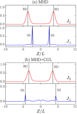
Figure 9: A cross-sectional view of current density at time $t=600L/V_{A}$ along $X=100L$. The top and bottom panels show the components parallel and perpendicular to the background magnetic field, respectively. (a) shows MHD, and (b) MHD + CGL.

We can also analyze hodograms of the magnetic field along the $Z$-axis at $X=100L$ in Fig. 10. The hodograms in (a)MHD and (b)MHD+CGL calculations are obtained from the same initial condition with $\phi=30^{\circ}$. The solid lines indicate simulation data, and the dashed lines equi-magnetic-energy circles. The outer and inner circles in both panels correspond to the magnetic energy upstream and downstream of slow shocks.

In the isotropic MHD case, the rotational waves rotate the magnetic field until $B_{X}$ becomes nearly equal to zero, and the slow shocks release the magnetic energy through the reduction of $B_{Y}$. In the MHD+CGL case, on the other hand, the slow shocks occur before the rotation of the magnetic field begins. Furthermore, the amount of magnetic energy released across the shocks in the MHD+CGL case (i.e., the width between the two equi-magnetic-energy circles) is much smaller than that in MHD case. These features are consistent with the steady state reconnection layer predicted by the 1-D Riemann problem (See Fig. 2).

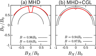
Figure 10: Hodograms of the magnetic field at time $t=600L/V_{A}$ along $X=100L$. The solid lines indicate simulation data and the dashed lines show equi-magnetic-energy circles. (a) is the isotropic MHD case and (b) the anisotropic MHD case (MHD + CGL).

The velocity profile is also modified by the pressure anisotropy. A snapshot of the flow velocity at time $t=600L/V_{A}$ is shown in Fig. 11. The color contour indicates the out-of-plane velocity, $V_{Y}$, and the vector map signifies the in-plane velocity vector, $(V_{X},V_{Z})$, normalized by $V_{A}$. The length of an arrow of $20L$ corresponds to $1V_{A}$. The boundary layers where the finite $V_{Y}$ arise are almost identical to the positions of rotational discontinuities. The plasma advected from the lobe region is accelerated to the $X$-direction across the boundary layer until an order of the ${\rm Alfv\acute{e}n}$ velocity. The outflow speed measured at $\left(X,Z\right)=\left(100L,0\right)$ reaches $0.76V_{A}$. In our isotropic MHD simulation (not shown here), the outflow speed measured at $(X,Z)=(100L,0)$ reaches $0.78V_{A}$, which is slightly less than the value $V_{A}\cos\phi=0.86V_{A}$, The outflow speed in the MHD+CGL case is smaller than an ordinary ${\rm Alfv\acute{e}n}$ velocity, $V_{A}\cos\phi$, and than that in the isotropic MHD case, but larger than a modified ${\rm Alfv\acute{e}n}$ velocity, $V_{A}^{*}\cos\phi=\sqrt{\varepsilon}V_{A}\cos\phi=0.58V_{A}$ calculated from the downstream anisotropy parameter. In 1-D simulations, it is assumed that all variables are uniform in the $X$-direction, but here in 2-D cases, non-uniformity along $X$-axis somewhat reduces the outflow velocities both in the isotropic and the anisotropic cases.

By measuring the inflow velocity at the point $(X,Z)=(0,50L)$, we found that the reconnection rates are $M_{A}=0.028$ in the MHD case, and $M_{A}=0.035$ in the MHD+CGL case. The ratio between these reconnection rates is $1.25$, and this is consistent with 1-D simulation results, discussed in previous section (see Fig. 6).

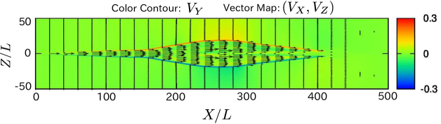
Figure 11: A snapshot of the MHD+CGL simulation with $\phi=30^{\circ}$ at time $t=600L/V_{A}$. The color contour shows the out-of-plane velocity, $V_{Y}$, normalized by the ${\rm Alfv\acute{e}n}$ velocity in the lobe region, $V_{A}$, and the vector map shows the in-plane components, $(V_{X},V_{Z})$. The length of an arrow of $20L$ corresponds to $1V_{A}$.

IV Discussion and Conclusion

We summarize the main results obtained from the 1-D and 2-D simulations as follows:

1. Once magnetic reconnection takes place, a pair of slow shocks does form even in an anisotropic MHD.

2. The parallel pressure increases mainly across the slow shock, and the large pressure anisotropy is induced.

3. The generated slow shocks are much weaker than those formed in an isotropic MHD, from the aspects of the compression ratio and the amount of released magnetic energy.

4. In spite of the weakness of the slow shocks, the resultant reconnection rate is $10-30\%$ larger than that in an isotropic MHD.

Result 1 is verified by comparing the downstream variables with theoretical values predicted by the Rankine-Hugoniot relations in anisotropic plasmas,Karimabadi1995 ; Chao1970 ; Hudson1971 in which a downstream anisotropy parameter $\varepsilon_{2}$ is treated as a given parameter obtained from the simulation data. From the point of view of the fluid approximation, as Petschek pointed out, magnetically stored energy is actually converted to thermal and kinetic energy in plasmas through the formation of a pair of slow shocks even under the pressure anisotropy. The modification from the reconnection layers in isotropic fluids is mentioned in Results 2-4.

Result 2 is a straightforward outcome of the double adiabatic theory, as mentioned in Section II. This result may correspond to the microscopic view of the plasma sheet boundary layer, such that the PSBL ion beam accelerated along the background magnetic field distorts the distribution function in kinetic regime.Higashimori2012 The second order momentum of the distribution function suggests $p_{||}>p_{\perp}$.

The downstream anisotropy parameter, $\varepsilon_{2}$, strongly depends on both the shear angle of the field lines, $\phi$, and the upstream plasma beta, but when $\phi$ approaches $0^{\circ}$, $\varepsilon_{2}$ becomes nearly $0$, which corresponds to the marginal firehose criterion. According to previous kinetic simulations, Liu2011a ; Liu2011b however, the downstream anisotropy parameter is somewhat larger than $0$. These authors argue that the ${\rm Alfv\acute{e}nic}$ counter-streaming ions, here corresponding to the parallel pressure enhancement, drive the drop of $\varepsilon_{2}$, and that downstream turbulent waves with the ion inertial scale scatter particles and raise $\varepsilon_{2}$. Since there is no counterpart of inertial scale waves in our simulations, it is consistent that $\varepsilon_{2}$ falls to a value smaller than that in the kinetic simulations. Comparisons between the 1-D and 2-D calculations show that $\varepsilon_{2}$ obtained in the 2-D case is slightly larger than the corresponding 1-D value, at least for $\phi$ larger than $20^{\circ}$. The multi-dimensionality, or non-uniformity in the $X$-direction, may also be essential for the development of the anisotropy in reconnection.

Results 3 and 4 are the most significant results in this work. Despite the smallness of the amount of magnetic energy released only across the slow shocks, the reconnection rates are maintained or slightly increase in the MHD+CGL calculations. Due to a relatively small enhancement of perpendicular pressure, pressure equilibrium related to $p_{\perp}+B^{2}/8\pi$ cannot be maintained, and the current sheet is squashed. This unbalance tends to enlarge the inflow velocities and the reconnection rates. Furthermore, the acceleration of reconnection exhaust is realized not only by the weak slow shocks, but also by the rotational discontinuities, which is striking especially for relatively small guide field reconnection. Note that the similar results have been obtained in the isotropic MHD Tsai2006 .

Finally, our results may be able to explain the rareness of the in-situ observations of the Petschek-type reconnection accompanied by slow shocks. The slow shocks formed in a collisionless magnetic reconnection might be too weak to be observed in their own right. Moreover, not only in the isotropic MHDTsai2006 , but also in the anisotropic MHD, the results imply that the slow shocks do not necessarily play an important role in the energy conversion in the collisionless magnetic reconnection system.

- (1) N. Sckopke, G. Paschmann, G. Haerendel, B. U. O. Sonnerup, S. J. Bame, T. G. Forbes, E. W. J. Hones, and C. T. Russell, JGR 86, 2099 (1981).
- (2) M. Hesse and D. Winske, JGR 99, 11177 (1994).
- (3) H. U. Frey., T. D. Phan, S. A. Fuselier, and S. B. Mende, Nature 426, 533 (2003).
- (4) M. Øieroset, T. D. Phan, M. Fujimoto, R. P. Lin, and R. P. Lepping, Nature 412, 414 (2001).
- (5) T. Nagai, I. Shinohara, M. Fujimoto, M. Hoshino, Y. Saito, S. Machida, and T. Mukai, JGR 106, 25929 (2001).
- (6) S. Zenitani, I. Shinohara, and T. Nagai, JGR 39, L11102 (2012).
- (7) E. N. Parker, ApJS 8, 177 (1963).
- (8) R. A. Kopp and G. W. Pneuman, Solar Physics 50, 85 (1976).
- (9) S. Masuda, T. Kosugi, H. Hara, S. Tsuneta, and Y. Ogasawara, Nature 371, 495 (1994).
- (10) P. A. Sweet, IAU Symposium No.6 Electromagnetic Phenomena in Ionized Gases (1958), p. 123, Stockholm.
- (11) E. N. Parker, Phys.Rev. 107, 830 (1957).
- (12) H. E. Petschek, NASA Spac. Publ. 50, 425 (1964).
- (13) Y. Saito, T. Mukai, T. Terasawa, A. Nishida, S. Machida, M. Hirahara, K. Maezawa, S. Kokubun, and T. Yamamoto, JGR 100, 23567 (1995).
- (14) J. Seon, L. A. Frank, W. R. Paterson, J. D. Scudder, F. V. Coroniti, S. Kokubun, and T. Yamamoto, JGR 101, 27383 (1996).
- (15) Y.-H. Liu, J. F. Drake, and M. Swisdak, Phys. Plasmas 18, 062110 (2011).
- (16) K. Higashimori and M. Hoshino, JGR 117, A01220 (2012).
- (17) C. J. Weng, C.C. Lin, L. C. Lee, and J. K. Chao, Phys. Plasmas 19, 122904 (2012).
- (18) M. Hoshino, T. Mukai, T. Yamamoto, and S. Kokubun, JGR 103, 4509 (1998).
- (19) M. Hoshino, T. Mukai, I. Shinohara, Y. Saito, and S. Kokubun, JGR 105, 337 (2000).
- (20) R. M. Kulsrud, “Handbook of plasma physics,” (North Holland, New York, 1983) Chap. 1.4.
- (21) G. F. Chew, M. L. Goldberger, and F. E. Low, Proc. R. Soc. London, Ser. A 236, 112 (1956).
- (22) G. W. Hammett and F. W. Perkins, Phys. Rev. Lett. 64, 3019 (1990).
- (23) G. W. Hammett, W. Dorland, and F. W. Perkins, Phys. Fluid B 4, 2052 (1992).
- (24) P. B. Snyder, G. W. Hammett, and W. Dorland, Phys. Plasmas 4, 3974 (1997).
- (25) P. Sharma, G. W. Hammett, E. Quataert, and J. M. Stone, ApJ 637, 952 (2006).
- (26) M. Rempel, M. Schüssler, and M. Knölker, ApJ 691, 640 (2009).
- (27) C. L. Tsai, L. C. Lee, and B. H. Wu, Phys. Plasmas 13, 102902 (2006).
- (28) M. F. Heyn, H. K. Biernat, R. P. Rijnbeek, and V. S. Semenov, Journal of Plsama Phys. 40, 235 (1988).
- (29) H. Karimabadi, D. Krauss-Varban, and N. Omidi, Geophys. Res. Lett. 22, 2689 (1995).
- (30) J. K. Chao, CSR TR-70-3 Center for Space Research, Massachusetts Institute of Technology(1970).
- (31) P. D. Hudson, Planet. Space Sci 19, 1693 (1971).
- (32) Y.-H. Liu, J. F. Drake, and M. Swisdak, Phys. Plasmas 18, 092102 (2011).