Global Solar Free Magnetic Energy and Electric Current Density Distribution of Carrington Rotation 2124

Abstract

Solar eruptive phenomena, like flares and coronal mass ejections(CMEs) are governed by magnetic fields. To describe the structure of these phenomena one needs information on the magnetic flux density and the electric current density vector components in three dimensions throughout the atmosphere. However, current spectro-polarimetric measurements typically limit the determination of the vector magnetic field only to the photosphere. Therefore, there is considerable interest in accurate modeling of the solar coronal magnetic field using photospheric vector magnetograms as boundary data. In this work, we model the coronal magnetic field for global solar atmosphere using a nonlinear force-free field(NLFFF) extrapolation codes implemented to a synoptic maps of photospheric vector magnetic field synthesized from Vector Spectromagnetograph (VSM) on Synoptic Optical Long-term Investigations of the Sun (SOLIS) as boundary condition. Using the resulting three dimensional magnetic field, we calculate the three dimensional electric current density and free magnetic energy throughout the solar atmosphere for Carrignton rotation 2124. We found that spatially, the low-lying, current-carrying core field demonstrates strong concentration of free energy in the AR core, from the photosphere to the lower corona; the coronal field becomes slightly more sheared in the lowest layer and it relaxes to the potential field configuration with height. The free energy density appears largely co-spatial with the electric current distribution.

1 Introduction

Extreme solar activity is powered by magnetic energy [Forbes (2000)]. Therefore, our understanding of the energy storage and release mechanism of solar eruptive events is strongly dependent on knowledge of their magnetic field configurations [Valori, Kliem, and Keppens (2005), Wiegelmann and Sakurai (2012)]. Flux emergence and shearing motion may introduce strong electric currents and inject energy to the active region (AR) corona. Nonpotential magnetic field topology carries electric current and free magnetic energy. Free magnetic energy is one of the main indicators used in space weather forecast to predict the eruptivity of active regions, and it can be converted into kinetic and thermal energies as the result of eruption[Régnier and Priest (2007a)]. Therefore, the three-dimensional (3D) structure of magnetic fields and electric currents in the pre-eruptive corona volume, are requirements to study those eruptive solar events. Thus the detailed aspects of the coronal field like twist, shear, loop structure, and connectivity have to be known to a high degree of accuracy. Unfortunately, due to the extremely low density and high temperature of the corona, measurements of the magnetic field are restricted to lower layers of the solar atmosphere. Although measurements of magnetic fields in the chromosphere and the corona have been considerably improved in recent decades [Lin, Penn, and Tomczyk (2000), Liu and Lin (2008)], further developments are needed before accurate data are routinely available. Another problem with these methods is that they do not provide the field in 3D and the measurements have a line-of-sight integrated character [Judge, Habbal, and Landi (2013)]. As an alternative to direct measurement of the three dimensional coronal magnetic field, numerical modeling are used to infer the field strength in the higher layers of the solar atmosphere from the measured photospheric magnetic field.

Due to the low value of the ratio of gas pressure to magnetic pressure (plasma $\beta$ ), the solar corona is magnetically dominated and the field is not affected by the plasma that it carries. The coronal field is often said to be force-free, i.e., free of forces other than the balancing electromagnetic forces that it exerts on itself [Gary (2001)]. Force-free condition assumes that the corona is static and free of Lorentz forces. This means that any electric currents must be aligned with the magnetic field. Force-free coronal magnetic fields are defined entirely by requiring that the field has no Lorentz force and is divergence free (the solenoidal condition):

$$(\nabla\times\textbf{B})\times\textbf{B}=0\ilabel{one}$$ (1)

$$\nabla\cdot\textbf{B}=0\ilabel{two}$$ (2)

where B is the magnetic field. Equation (one) states that the Lorentz force vanishes (as a consequence of $\textbf{J}\parallel\textbf{B}$, where J is the electric current density) and Equation (two) describes the absence of magnetic monopoles. Using Equations (one) and (two) as constraints equations, one can calculate the magnetic field density in a corona volume for photospheric measurements. Nonlinear force-free magnetic field (NLFFF) extrapolation techniques are the best mathemathical modeling tools currently being used to estimate the magnetic field in the higher solar atmosphere [Amari and Aly (2010), Aschwanden and Malanushenko (2012), Contopoulos (2013), He and Wang (2008), Malanushenko et al. (2012), Jiang and Feng (2012), Song et al. (2007), Tadesse, Wiegelmann, and Inhester (2009), Tadesse et al. (2013a), Wheatland, Sturrock, and Roumeliotis (2000), Wheatland and Régnier (2009), Wiegelmann (2004), Wiegelmann (2007)]. For more detailed explanations of NLFFF methods, we direct the reader to the recent review by Wiegelmann:2012W.

Electric currents are thought to play an important role for the energetics of the chromosphere and the corona of the Sun. Twisted magnetic field line implies the presence of field-aligned electric currents (but see h=80Mm:1997 for counter example of potential field lines that appear highly sheared). The existence of electric currents implies departure of the magnetic structure from its minimum-energy, current-free (potential) configuration. Therefore, free magnetic energy is associated with electric currents flowing in the solar corona. Having the three-dimensional structure of the vector magnetic field, one can compute the vector current density as the curl of the field. On the largest scales, the corona of a whole hemisphere was found to be magnetically coupled [Schrijver (2009), h=80Mm and Acton (2001)]. Therefore, it appears prudent to implement a NLFFF procedure in spherical geometry [Amari et al. (2013), Tadesse et al. (2013b)] for use when global scale boundary data are available (see Figure fig1), such as synoptic maps of photospheric vector magnetic field synthesized from Vector Spectromagnetograph (VSM) on Synoptic Optical Long-term Investigations of the Sun (SOLIS) [Gosain et al. (2013)]. In this work, we apply spherical NLFFF procedure to synoptic vector map of Carrington rotation 2124 to reconstruct 3D magnetic field solutions (potential and NLFFF) from which we infer the distributions of free magnetic energy and electric current density in corona volume globally.

2 Optimization Procedure for Global Nonlinear Force-Free Field Model

Wheatland:2000 derived an optimization approach based on a pseudo-energy integral which is minimized by a divergence-free, force-free field [Equations (one) and (two)] using Cartesian geometry. The variation of the integral with respect to the variation of the magnetic field gives a pseudo-force, which can be used to dynamically drive the system from a potential field toward a force-free field that minimizes the pseudo-energy integral, subject to the required boundary conditions at the photospheric level. The optimization method requires that the magnetic field is given on all (6 for a rectangular computational box) boundaries. This causes a serious limitation of the method because such data are only available for model configurations. Later on, Wiegelmann:2004 improved the method in a such away that it can reconstruct the magnetic field only from photospheric vector magnetograms by diminishing the effect of the top and lateral boundaries on the magnetic field inside the computational box.

Since extrapolation codes of Cartesian geometry for medelling the magnetic field in the corona do not take the curvature of the Sun’s surface into account, Wiegelmann:2007 extended the method into spherical coordinates in a such way that it can handle the the Sun, globally. Later on, Tadesse:2009 developed code for the extrapolation of nonlinear force-free coronal magnetic fields in spherical coordinates over a restricted area of the Sun [Tadesse et al. (2012a), Tadesse et al. (2012b), Tadesse et al. (2013c)]. In this work, we use the optimization procedure for functional $L$ in spherical geometry for the whole Sun globaly [Wiegelmann (2007), Tadesse, Wiegelmann, and Inhester (2009)], which enforces a minimal deviation between the photospheric boundary of the model field B and the measured field value $\textbf{B}_{\rm obs}$ by adding an appropriate surface integral term $L_{\rm photo}$ [Wiegelmann and Inhester (2010), Tadesse et al. (2011)] as in the following equation:

$$L=L_{\rm f}+L_{\rm d}+\nu L_{\rm photo}\ilabel{4}$$ (3)

$$L_{\rm f}=\int_{V}B^{-2}\big{|}(\nabla\times{\textbf{B}})\times{\textbf{B}}\big{|}^{2}r^{2}\sin\theta drd\theta d\phi$$

$$L_{\rm d}=\int_{V}\big{|}\nabla\cdot{\textbf{B}}\big{|}^{2}r^{2}\sin\theta drd\theta d\phi$$

$$L_{\rm photo}=\int_{S}\big{(}\textbf{B}-\textbf{B}_{\rm obs}\big{)}\cdot\textbf{W}(\theta,\phi)\cdot\big{(}\textbf{B}-\textbf{B}_{\rm obs}\big{)}r^{2}\sin\theta d\theta d\phi$$

where $L_{\rm f}$ and $L_{\rm d}$ measure how well the force-free equation [Equation (one)] and divergence-free condition [Equation (two)] are fulfilled, respectively. We implement the surface integral term, $L_{\rm photo}$, in Equation (4) to work with boundary data of different noise levels and qualities [Wiegelmann and Inhester (2010), Tadesse et al. (2011)]. This allows deviations between the model field B and the input field, i.e. the observed $\textbf{B}_{\rm obs}$ surface field, so that the model field can be iterated closer to a force-free solution. $\textbf{W}(\theta,\phi)$ is a space-dependent diagonal matrix whose elements $(w_{los},w_{trans},w_{trans})$ are inversely proportional to the estimated squared measurement error of the respective field components. Because the line-of-sight photospheric magnetic field is measured with much higher accuracy than the transverse field, we typically set the component $w_{los}$ to unity, while the transverse components of $w_{trans}$ are typically small but positive. In regions where transverse field has not been measured or where the signal-to-noise ratio is very poor, we set $w_{trans}=0$. In order to control the speed with which the lower boundary condition is injected during the NLFFF extrapolation, we have used the Lagrangian multiplier of $\nu=0.001$ as suggested by Tadesse:2013.

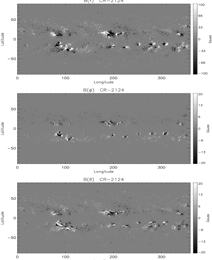
Figure 1.: Synoptic Carrington maps of the vector magnetic field components are shown for CR-2124. The panels from top to bottom show the distribution of the $B(r)$, $B(\phi)$ and $B(\theta)$ components, respectively. The $B_{r}$ map is scaled between $\pm$ 100 G, and the $B_{\phi}$ and $B_{\theta}$ maps are scaled to $\pm$ 20 G. The positive values of $B_{r}$, $B_{\phi}$ and $B_{\theta}$ point, respectively, upward, to the right (westward) and southward.fig1

We use spherical preprocessing procedure to remove most of the net force and torque from the synoptic vector data so that the boundary can be more consistent with the force-free assumption [Wiegelmann, Inhester, and Sakurai (2006), Tadesse, Wiegelmann, and Inhester (2009)]. The potential field solution has been used to initialize NLFFF code. To calculate NLFFF solutions, we minimize the functional given by Equation (4) using preprocessed photospheric boundary data. We use a uniform spherical grid $r$, $\theta$, $\phi$ with $n_{r}=225$, $n_{\theta}=375$, and $n_{\phi}=425$ grid points in the direction of radius, latitude, and longitude, respectively. We aim to compute the whole sphere with the field of view of $[r_{\rm{min}}=1R_{\odot}:r_{\rm{max}}=1.5R_{\odot}]\times[\theta_{\rm{min}}=-90^{\circ}:\theta_{\rm{max}}=90^{\circ}]\times[\phi_{\rm{min}}=0^{\circ}:\phi_{\rm{max}}=360^{\circ}]$. To avoid the mathematical singularities at the poles, we do not use grid points exactly at the south and north pole, but set them half a grid point apart at $\theta_{min}=-90^{\circ}+d\theta/2$ and $\theta_{max}=90^{\circ}-d\theta/2$ (see, Wiegelmann:2007).

3 Results

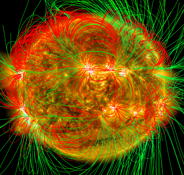
Figure 2.: Global field lines of the NLFFF model overlaid on the AIA 171Å image. Green and red lines represent open and closed magnetic field lines, respectively.fig2

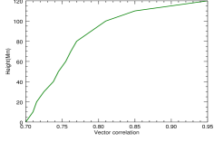
(a)

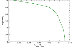
(b)

Figure 3.: (a) Plot of height variations of surface vector correlation between the potential field and NLFFF solutions. (b) Plot of height variations of ratio of free magnetic energy to potential magnetic energy.fig3

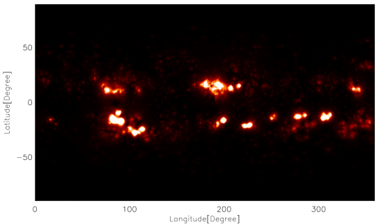
(a)

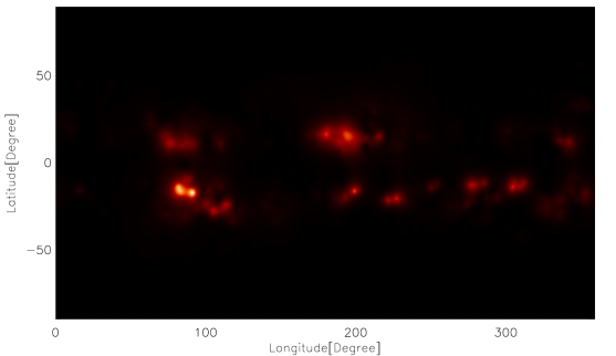
(b)

Figure 4.: Synoptic maps of the global free magnetic energy relative to the potential energy at (a) $h=0$ (photosphere) and (b) at $h=80Mm$ from the photosphere.fig4

In this section we apply the spherical optimization procedure to synoptic maps of photospheric vector magnetic field synthesized from Vector Spectromagnetograph (VSM) on Synoptic Optical Long-term Investigations of the Sun (SOLIS). The main purpose of this work is to study the distributions of free magnetic energy and electric current density in the global corona for Carrington rotation 2124 (May 2012 – June 2012) using NLFFF extrapolation. Two physical measures, the free magnetic energy and electric current density were calculated from the extrapolated fields to quantitatively evaluate the structure of the reconstructed 3D magnetic field for global corona.

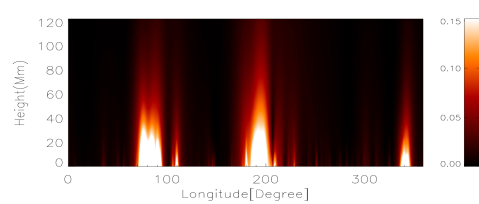
Figure 5.: Free magnetic energy density map on the latitudinal plane $\theta=15^{\circ}$ for global NLFFF field relative to potential field (increasing density from black to white).fig5

3.1 Global Free Magnetic Energy

Once the 3D magnetic configuration is reconstructed, we first have to check if characteristic magnetic structures can be obtained in comparison with observations. Therefore, the field line configurations of the extrapolated magnetic fields are compared with an AIA 171 Å coronal loop observations in Figure fig2. The Figure shows the open and closed field lines of the extrapolated magnetic fields overlying the corresponding AIA image. The comparison shows that the field lines of the modeling fields generally agree with the coronal loop images. We now consider the distribution of the magnetic free energy based on the NLFFF extrapolation. The potential field is a minimum of magnetic energy for a given distribution of the vertical or radial magnetic field component on the photosphere [Aly (1984)]. Therefore there is no free magnetic energy, no shear and/or twisted field lines in a potential field configuration. For these reasons, the nonlinear force-free field is more adequate to describe better the nature of the corona as it contains free magnetic energy and sheared and twisted flux bundles. We estimate the free magnetic energy, the difference between the extrapolated NLFFF and the potential field with the same normal boundary conditions in the photosphere [Régnier and Priest (2007a), Régnier and Priest (2007b)]. The free magnetic energy is a measure of the magnetic energy that can be stored in the magnetic configuration or released during an eruptive or reconnection event. We therefore estimate the upper limit to the free magnetic energy associated with coronal currents of the form

$$E_{\mathrm{free}}=\frac{1}{8\pi}\int_{V}\Big{(}B_{\rm nlff}^{2}-B_{\rm pot}^{2}\Big{)}r^{2}\sin\theta drd\theta d\phi,\ilabel{ten}$$ (4)

where $B_{\rm nlff}$ and $B_{\rm pot}$ are NLFFF and potential field solutions, respectively. Our result for the estimation of free-magnetic energy shows that the NLFFF model has $15\%$ more energy than the corresponding potential field model calculated from the same radial field boundary.

In order to quantify the degree of deviations between the potential and NLFFF vector field solutions in the global corona volume, we use the vector correlation metric ($C_{\rm vec}$) which is also used analogous to the standard correlation coefficient for scalar functions. The correlation was calculated [Schrijver et al. (2006)] from

$$C_{\mathrm{vec}}=\frac{\sum_{i}\textbf{v}_{i}\cdot\textbf{u}_{i}}{\Big{(}\sum_{i}|\textbf{v}_{i}|^{2}\sum_{i}|\textbf{u}_{i}|^{2}\Big{)}^{1/2}},\ilabel{6}$$ (5)

where $\textbf{v}_{i}$ and $\textbf{u}_{i}$ are the vectors at each grid point $i$. If the vector fields are identical, then $C_{\rm vec}=1$; if $\textbf{v}_{i}\perp\textbf{u}_{i}$ , then $C_{\rm vec}=0$. We calculated vector correlations of the potential and NLFFF solutions at different layers in corona volume and found that the correlation increases with height (see, Figure fig3a). The result shows that the coronal field loop becomes slightly more sheared in the lowest layer, relaxes to the potential field configuration with height. Similarly we calculated the ratio of total surface free magnetic to potential field energy over different layers in corona volume globally and found that the ratio decreases with height as shown in Figure fig3b. For illustration, we plot total surface free magnetic energy relative to the potential one at two layers. Figures fig4(a) and (b) show the contour plots of the global free magnetic energy relative to the potential energy on the photosphere and on the layer at height $h=80Mm$ above the photosphere, respectively. In Figure fig5 we plot the free magnetic energy density on the latitudinal plane $\theta=15^{\circ}$ for global NLFFF field relative to potential field and we found that spatially, the low-lying, current-carrying core field demonstrates strong concentration of free energy in the AR core, from the photosphere to the lower corona.

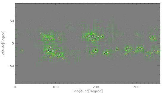
(a)

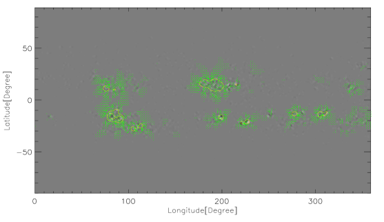
(b)

Figure 6.: Synoptic maps of electric current density distributions at (a) $h=0$ (photosphere) and (b) $h=80Mm$ from the photosphere. The color coding and the green arrows show $J_{r}$ and transverse components of electric current densities, respectively. The contour lines indicate the locations of free magnetic energy concentration.fig6

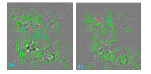
Figure 7.: Surface electric current density distributions at (a) $h=0$ (photosphere) and (b) $h=80Mm$ from the photosphere. The color coding and the green arrows show $J_{r}$ and transverse components of electric current densities, respectively. fig7

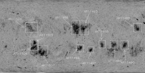
Figure 8.: He10830 synoptic map for Carrington Rotation 2124.fig8

3.2 Electric Current Density Distribution

Electric current systems are key component in understanding solar activity. Free magnetic energy is thought to derive from the non-potential component of the magnetic field, which is the part associated with electric currents flowing in the solar corona. Thus, free magnetic energy is directly connected to the magnitude of the electric currents in the solar atmosphere. Having the three-dimensional structure of the vector magnetic field, one can compute the vector current density J as the curl of the field:

$$\textbf{J}=\frac{1}{4\pi}\nabla\times\textbf{B},\ilabel{7}$$ (6)

where B is nonlinear force-free 3D magnetic field solution. We use finite difference method to solve for the electric current density from curl of $B$. We plot electric current density vector J at two different heights in Figure fig6. Figures fig6(a) and (b) show the contour plots of the global free magnetic energy and electric current densities on the photosphere and on the layer at height $h=80Mm$ above the photosphere, respectively. Figure fig6 shows that free energy density appears largely co-spatial with the current distribution. There is high free energy concentration above polarity inversion lines (PILs). In Figure fig7 shows zooming of the electric current densities of group of active regions located on the left side of Figures  fig6a). and b). It shows that the radial and transverse components of the current densities decrease at $h=80Mm$ height from the photosphere.

4 Discussion

In this study, we have investigated the distributions free magnetic energy and electric current density associated with nonlinear force-free global magnetic field in the corona by analyzing synoptic maps of photospheric vector magnetic field synthesized from Vector Spectromagnetograph (VSM) on Synoptic Optical Long-term Investigations of the Sun (SOLIS). The Carrington rotation number for this observation is 2124, which has been observed during 26th March - 21st June, 2012. We have used spherical NLFFF to compute the magnetic field solutions over global corona.

We have compared the NLFFF magnetic field solutions with the observed corresponding EUV loops. The comparison shows that the field lines of the modeling fields generally agree with the coronal loop images. For this particular Carrington rotation we found that the free magnetic energy density is $15\%$ of the potential one and spatially, the low-lying, current-carrying core field demonstrates strong concentration of free energy in the AR core, from the photosphere to the lower corona. One can compare the distribution of non-potential energy with coronal brightness integrated over selected active regions. In this comparison, we use synoptic map of equivalent width of spectral line He 1083.0 nm (low solar corona) from SOLIS/VSM (Figure fig8). Visually, active regions with the largest density of free energy (per unit area) at 80Mm are AR11504, AR11496, and AR11494 (see, brightest pixels in Figure fig4b). These active regions also exhibit the strongest equivalent width in Figure fig8. This suggests that active regions with largest amount of non-potential energy are brighter in the corona. In this study, the free energy density appears largely co-spatial with the current density distribution and the coronal field loop becomes slightly more sheared in the lowest layer, relaxes to the potential field configuration with height. By comparing Figures fig7a and b one can see that the patterns of electric currents are similar in the photosphere and 80Mm above it. These is no indication that the currents spread over larger area higher in atmosphere, while the amplitude of $J$-total clearly decreases with height. This decrease in amplitude of electric currents is in agreement with our conclusion that the magnetic field became more potential with height. It also indicates that the electric currents dissipate strongly with atmospheric height, and that there is no continuity of J through solar atmosphere. Photospheric electric currents are strongest in AR11504 and AR11497 (see Figure fig6a). On the other hand, the coronal brightness of AR11497 is not as high as in AR11504. This suggests only a weak correlation between the photospheric electric currents and the coronal brightness in agreement with Fisher:1998.

References

- Aly (1984) Aly, J.J.: 1984,. Astrophys. J. 283, 349.
- Amari and Aly (2010) Amari, T., Aly, J.J.: 2010,. Astron. Astrophys. 522, A52.
- Amari et al. (2013) Amari, T., Aly, J.J., Canou, A., Mikic, Z.: 2013,. Astron. Astrophys. 553, A43.
- Aschwanden and Malanushenko (2012) Aschwanden, M.J., Malanushenko, A.: 2012,. Solar Phys. doi:10.1007/s11207-012-0070-1.
- Contopoulos (2013) Contopoulos, I.: 2013,. Solar Phys. 282, 419.
- Fisher et al. (1998) Fisher, G.H., Longcope, D.W., Metcalf, T.R., h=80Mm, A.A.: 1998,. Astrophys. J. 508, 885.
- Forbes (2000) Forbes, T.G.: 2000,. J. Geophys. Res. 105, 23153.
- Gary (2001) Gary, G.A.: 2001,. Solar Phys. 203, 71.
- Gosain et al. (2013) Gosain, S., h=80Mm, A.A., Rudenko, G.V., Anfinogentov, S.A.: 2013,. Astrophys. J. 772, 52.
- He and Wang (2008) He, H., Wang, H.: 2008,. J. Geophys. Res. 113, 5.
- Jiang and Feng (2012) Jiang, C., Feng, X.: 2012,. Solar Phys. 281, 621.
- Judge, Habbal, and Landi (2013) Judge, P.G., Habbal, S., Landi, E.: 2013, From Forbidden Coronal Lines to Meaningful Coronal Magnetic Fields. Solar Phys. doi:10.1007/s11207-013-0309-5.
- Lin, Penn, and Tomczyk (2000) Lin, H., Penn, M.J., Tomczyk, S.: 2000,. Astrophys. J. Lett. 541, L83.
- Liu and Lin (2008) Liu, Y., Lin, H.: 2008,. Astrophys. J. 680, 1496.
- Malanushenko et al. (2012) Malanushenko, A., Schrijver, C.J., DeRosa, M.L., Wheatland, M.S., Gilchrist, S.A.: 2012,. Astrophys. J. 756, 153.
- h=80Mm and Acton (2001) h=80Mm, A.A., Acton, L.W.: 2001,. Astrophys. J. 554, 416.
- h=80Mm, Canfield, and McClymont (1997) h=80Mm, A.A., Canfield, R.C., McClymont, A.N.: 1997,. Astrophys. J. 481, 973.
- Régnier and Priest (2007a) Régnier, S., Priest, E.R.: 2007a,. Astrophys. J. Lett. 669, L53.
- Régnier and Priest (2007b) Régnier, S., Priest, E.R.: 2007b,. Astron. Astrophys. 468, 701.
- Schrijver (2009) Schrijver, C.J.: 2009,. Adv. Space Res. 43, 739.
- Schrijver et al. (2006) Schrijver, C.J., De Rosa, M.L., Metcalf, T.R., Liu, Y., McTiernan, J., Régnier, S., Valori, G., Wheatland, M.S., Wiegelmann, T.: 2006,. Solar Phys. 235, 161.
- Song et al. (2007) Song, M.T., Fang, C., Zhang, H.Q., Tang, Y.H., Wu, S.T., Zhang, Y.A.: 2007,. Astrophys. J. 666, 491.
- Tadesse, Wiegelmann, and Inhester (2009) Tadesse, T., Wiegelmann, T., Inhester, B.: 2009,. Astron. Astrophys. 508, 421.
- Tadesse et al. (2011) Tadesse, T., Wiegelmann, T., Inhester, B., h=80Mm, A.: 2011,. Astron. Astrophys. 527, A30.
- Tadesse et al. (2012a) Tadesse, T., Wiegelmann, T., Inhester, B., h=80Mm, A.: 2012a,. Solar Phys. 281, 53.
- Tadesse et al. (2012b) Tadesse, T., Wiegelmann, T., Inhester, B., h=80Mm, A.: 2012b,. Solar Phys. 277, 119.
- Tadesse et al. (2013a) Tadesse, T., Wiegelmann, T., Inhester, B., MacNeice, P., h=80Mm, A., Sun, X.: 2013a,. Astron. Astrophys. 550, A14.
- Tadesse et al. (2013b) Tadesse, T., Wiegelmann, T., MacNeice, P.J., Olson, K.: 2013b,. Astrophys. and Space Science 347, 21.
- Tadesse et al. (2013c) Tadesse, T., Wiegelmann, T., MacNeice, P.J., Olson, K.: 2013c,. Astrophys. and Space Science 348, 21.
- Valori, Kliem, and Keppens (2005) Valori, G., Kliem, B., Keppens, R.: 2005,. Astron. Astrophys. 433, 335.
- Wheatland and Régnier (2009) Wheatland, M.S., Régnier, S.: 2009,. Astrophys. J. Lett. 700, L88.
- Wheatland, Sturrock, and Roumeliotis (2000) Wheatland, M.S., Sturrock, P.A., Roumeliotis, G.: 2000,. Astrophys. J. 540, 1150.
- Wiegelmann (2004) Wiegelmann, T.: 2004,. Solar Phys. 219, 87.
- Wiegelmann (2007) Wiegelmann, T.: 2007,. Solar Phys. 240, 227.
- Wiegelmann and Inhester (2010) Wiegelmann, T., Inhester, B.: 2010,. Astron. Astrophys. 516, A107.
- Wiegelmann and Sakurai (2012) Wiegelmann, T., Sakurai, T.: 2012,. Living Rev. Solar Phys. 9, 5. http:// http://solarphysics.livingreviews.org/Articles/lrsp-2012-5/.
- Wiegelmann, Inhester, and Sakurai (2006) Wiegelmann, T., Inhester, B., Sakurai, T.: 2006,. Solar Phys. 233, 215.