The Linear Sigma Model and the formation of a charged pion condensate in the presence of an external magnetic field.

Abstract

We discuss the charged pion condensation phenomenon in the linear sigma model, in the presence of an external uniform magnetic field. The critical temperature is obtained as a function of the external magnetic field, assuming the transition is of second order, by considering a dilute gas at low temperature. As a result we found magnetic catalysis for high values of the external magnetic field. This behavior confirms previous results with a single charged scalar field.

I Introduction

In a recent article the occurrence of magnetic catalysis for the formation of a charged Bose-Einstein condensate was discussed in the frame of a self-interacting complex scalar field nuestro . It shows that, contrary to what was argued previously in the literature Schafroth ; May ; Toms:1992dq ; DFK ; Toms:1993ic ; Toms:1994cq ; Elmfors:1994mz , the realization, of a charged Bose-Einstein condensate is possible in 3 spatial dimensions in the presence of a uniform external magnetic field when screening effects are considered. The effects of external magnetic fields on charged bosons systems has been matter of discussion in several articles studying chiral symmetry restoration through the effective potential, including ressumation in the high temperature region ayalaetal ; cristiannuevo .

In the present article we concentrate on the formation of the charged pion condensate in the frame of the linear sigma mode, taking into account effects of a uniform external magnetic filed. Pion condensation could play a relevant role in the cooling process of compact stars Baym1 ; Stars and it has been extensively studied in different contexts as, for example chiral perturbation theory Kogut ; Villavicencio ; Verbaarschoot ; Son2 ; Kogut2 , the Nambu-Jona-Lasinio (NJL) model Zhao ; Munshi ; Ebert ; Ebert2 and other Quantum Chromodynamics (QCD) effective models Son ; Klein ; Toublan ; Barducci ; Barducci2 ; Son3 ; Splittdorff ; Herpay .

The linear sigma model exhibits many of the global symmetries of QCD. The model was originally introduced by Gell-Mann and Levy gellmann with the purpose of describing pion-nucleon interactions. During the last years an impressive amount of work has been done with this model. The idea is to consider it as an effective low energy approach for QCD. Its simplicity and beautiful realization, explicit as well as implicit, of chiral symmetry breaking has motivated people to consider it as a valuable tool for studying phase transitions. Actually, there are not many contributions in the literature about the linear sigma model in the presence of magnetic fields or when a pion superfluid condensate is taken into account. Shu and Li Shu have studied Bose-Einstein condensation and the chiral transition, in the chiral limit, within the linear sigma model. In Mizher , a discussion of the structure of the phase diagram in the presence of a magnetic background, in the framework of the linear sigma model, coupled to quarks and/or Polyakov loop has been presented. The effects of CP violation on the nature of the chiral transition within the linear sigma model with two flavors of quarks in a strong magnetic background has been discussed in Mizher2 . In He the occurrence of pion superfluidity at finite temperature and isospin chemical potential has been considered in the frame of the linear sigma model.

The main idea of the present article is to consider the effective potential at the one loop level, taking the isospin chemical potential near the effective pion mass, varying then the intensity of the magnetic field in order to obtain the critical temperature. Essentially we have followed the same procedures performed in nuestro , but this time in a more realistic model.

This article is organized as follows: In section II we present our model in the presence of an external magnetic field with a finite isospin chemical potential. We search for the lowest energy state where the pion condensate occurs, defining then our order parameter for the phase transition. In section III we proceed to calculate the effective potential at the one loop level. In section IV we calculate the relevant diagrams as well as the charge number density. In section V we explain the prescription adopted in order to fix the different parameters. In section VI, we present and explain our results which include the critical temperature for the charged pion condensation as a function of the magnetic field and the superfluid density as a function of the temperature. Finally we present our conclusions and outlook.

II The Model

In the Euclidean space, the Lagrangian of the linear sigma model, without a fermionic sector, but including isospin chemical potential and an external magnetic field is given by

$$S = \int_{\beta}dx\Big{[}(\partial_{4}-\mu_{I})\pi_{+}(\partial_{4}+\mu_{I})\pi_{-}$$ (1)

$$+(\partial_{i}-ieA_{i})\pi_{+}(\partial_{i}+ieA_{i})\pi_{-}$$

$$+\frac{1}{2}[(\partial\sigma)^{2}+(\partial\pi_{0})^{2}+\mu_{0}^{2}(\sigma^{2}+\pi_{0}^{2}+2\pi_{+}\pi_{-})]$$

$$+\frac{\lambda}{4}(\sigma^{2}+\vec{\pi}^{2})^{2}-c\sigma\Big{]},$$

where $\mu_{I}$ is the isospin chemical potential. $\pi_{+}$ and $\pi_{-}$ represent charged pion fields, $\pi_{0}$ is the neutral pion field and $\sigma$ is the field associated to the sigma meson. The integral is defined as

$$\int_{\beta}dx\equiv\int_{0}^{\beta}dx_{4}\int d^{3}x,$$ (2)

where $\beta=1/T$, being $T$ the temperature of the system. The term $c\sigma$ corresponds to the explicit chiral symmetry breaking term, being $c=f_{\pi}m_{\pi}^{2}$ and where $f_{\pi}=93.5MeV$ is the pion decay constant. In the symmetric gauge, the external gauge field which produces a uniform magnetic field in the $z$ direction can be written as

$$\vec{A}=\frac{1}{2}\vec{B}\times\vec{r}=\frac{1}{2}B(-x_{2},x_{1},0).$$ (3)

The symmetry is spontaneously and explicitly broken and, therefore, we assume that the expectation value of the sigma field $\bar{\sigma}$ has a non vanishing value. If we consider that the isospin symmetry is also broken due to the formation of the charged pion condensate, we can then expand the fields as quantum fluctuations around the classical fields. In the case of the $\sigma$ field, we will apply the mean field approximation. In the case of the pion fields, we take the classical field oriented in one isospin direction, conventionally in the $\pi_{1}$ direction:

$$\sigma(x)=\bar{\sigma}+\widetilde{\sigma}(x),\hskip 28.45274pt\pi_{\pm}(x)=\frac{1}{\sqrt{2}}\phi_{c}(x)+\widetilde{\pi}_{\pm}(x).$$ (4)

The mean field approximation cannot be applied to the classical pion field due to nontrivial coupling to the external magnetic field harrington . Therefore, in order to find the minimum value of the pion expectation value, a variational analysis has to be done.

Our analysis will concentrate in a region close to the formation of the superfluid pion phase. The effective action up to tree-level is

$$S_{cl} = \beta\int{d^{3}x}\bigg{\{}\frac{1}{2}\mu_{0}^{2}\bar{\sigma}^{2}+\frac{\lambda}{4}\bar{\sigma}^{4}-c\bar{\sigma}$$ (5)

$$+\frac{1}{2}(\partial_{i}\phi_{c})^{2}+\frac{1}{2}(m_{\pi}^{2}-\mu_{I}^{2}+e^{2}A_{i}^{2})\phi_{c}^{2}+\frac{\lambda}{4}\phi_{c}^{4}\bigg{\}},$$

where

$$m_{\pi}^{2}=\mu_{0}^{2}+\lambda\bar{\sigma}^{2}.$$ (6)

Minimizing with respect to $\phi_{c}$ the free part of the classical action, and then looking for eigenstates, we find that the classical field $\phi_{c}$ satisfies a kind of non-relativistic Schrödinger equation:

$$[-\nabla^{2}+(eB)^{2}(x_{1}^{2}+x_{2}^{2})/4+m_{\pi}^{2}-\mu_{I}^{2}]\phi_{c}=E^{2}\phi_{c}.$$ (7)

We immediately recognize in the previous equation the two-dimensional harmonic oscillator whose eigenvalues are

$$E_{l}^{2}(p_{z})=p_{z}^{2}+m_{\pi}^{2}+(2l+1)eB-\mu_{I}^{2}.$$ (8)

Since we are looking for the ground state of the classical pion field eigenvalues, we will consider the eigenfunction associated to $p_{z}=0$ and $l=0$. In this way we obtain brito

$$\phi_{c}=v_{0}e^{-eB(x_{1}^{2}+x_{2}^{2})/4},$$ (9)

where $v_{0}$ is a constant which happens to be the order parameter when the $B=0$. We define the order parameter for the formation of the pion condensate as

$$\bar{v}\equiv\left[\frac{1}{V}\int d^{3}x\phi_{c}^{2}\right]^{1/2},$$ (10)

where $V$ is the volume of the system. In terms of $\bar{v}$ the classical field reads

$$\phi_{c}=\bar{v}\left(\frac{1-e^{-\Phi/2\Phi_{0}}}{\Phi/2\Phi_{0}}\right)^{1/2}e^{-eB(x_{1}^{2}+x_{2}^{2})/4},$$ (11)

where $\Phi\equiv BA$ is the magnetic flux, $A$ is the area transverse to the external magnetic field and $\Phi_{0}\equiv\pi/q$ is the quantum magnetic flux. With this definition of the order parameter $\bar{v}$ it turns out that the tree-level effective mass is independent of the magnetic flux. A different prescription will produce a global flux dependent term.

If higher Landau levels are included in the classical description, if for some reason the true ground state is suppressed, then the formation of the superfluid phase will be more difficult and the critical chemical potential must be increased. However, since the true ground state is present, we may expect the appearance of quasiparticles in the spectrum asocciated to the interaction between pions in the superfluid phase and pions in the normal phase with higher Landau levels, according to Bogoliubov’s description Martin:2002uq .

III Effective potential up to 1-loop

Starting from our action in (1), we proceed to calculate the effective potential at the 1-loop order, which is given by:

$$\Omega=\frac{1}{\beta V}\left(S_{cl}+\frac{1}{2}Tr\ln D^{-1}\right),$$ (12)

where $S_{cl}$ is the classical action in Eq. (5), and the inverse propagator matrix operator is given by

$$D^{-1}=\begin{bmatrix}-\partial^{2}+m_{\sigma}^{2}+\lambda\phi_{c}^{2}&0&\sqrt{2}\lambda\bar{\sigma}\phi_{c}&\sqrt{2}\lambda\bar{\sigma}\phi_{c}\\ 0&-\partial^{2}+m_{\pi}^{2}+\lambda\phi_{c}^{2}&0&0\\ \sqrt{2}\lambda\bar{\sigma}\phi_{c}&0&-\mathcal{D}_{-}^{2}+m_{\pi}^{2}+2\lambda\phi_{c}^{2}&\lambda\phi_{c}^{2}\\ \sqrt{2}\lambda\bar{\sigma}\phi_{c}&0&\lambda\phi_{c}^{2}&-\mathcal{D}_{+}^{2}+m_{\pi}^{2}+2\lambda\phi_{c}^{2}\end{bmatrix}.$$ (13)

$m_{\sigma}^{2}=\mu_{0}^{2}+3\lambda\bar{\sigma}^{2}$, $m_{\pi}$ is defined in Eq. (6), and

$$\mathcal{D}_{\pm}^{2}=(\partial_{4}\pm\mu_{I})^{2}+(\partial_{i}\pm ieA_{i})^{2}.$$ (14)

As we said, we want to explore the condensation phenomenon close to the phase transition, assuming this is of second order. This means that the order parameter value will be close to the value in the normal phase, i.e. near $\bar{v}=0$. Therefore, we can expand the effective potential around the order parameter $\bar{v}=0$.

$$\Omega=\Omega_{0}+\frac{1}{2}\Omega_{2}\bar{v}^{2}+\frac{1}{4!}\Omega_{4}\bar{v}^{4}+\cdots.$$ (15)

where

$$\Omega_{n}=\left.\frac{\partial^{n}\Omega}{\partial\bar{v}^{n}}\right|_{\bar{v}=0}.$$ (16)

This assumption does not exclude the fact that a first order phase transition or a crossover may occur. However, here we will deal only with second order phase transitions which is actually the case at zero external magnetic field. In this scenario the value of $\bar{\sigma}$ that minimizes the effective potential will be

$$\frac{\partial\Omega_{0}}{\partial\bar{\sigma}}=0.$$ (17)

On the other hand, one of the observables is the charge number density which remains constant in the normal phase as well as in the superfluid phase. Therefore,

$$\rho=-\frac{\partial\Omega_{0}}{\partial\mu_{I}}.$$ (18)

For $\mu_{I}\leq\mu_{c}$ being $\mu_{c}(T_{c},\rho,B)$ the critical chemical potential where the condensation begins. The second order phase transition occurs when the effective pion mass term in the effective potential vanishes, i.e., when $\Omega_{2}\rightarrow 0$, whenever $\Omega_{4}>0$. The symmetric phase corresponds to $\Omega_{2}>0$ and the broken phase when $\Omega_{2}<0$. So the condition for the second order phase transition that fixes $\mu_{c}$ will be

$$\Omega_{2}=0.$$ (19)

This means that we only need to calculate the quantities $\Omega_{0}$ and $\Omega_{2}$ in the normal phase near the phase transition.

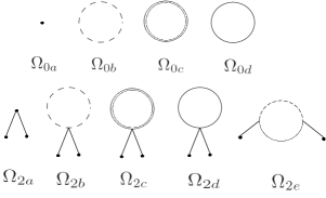
Figure 1: Relevant diagrams for the second derivative of the effective potential with respect to the order parameter $\bar{v}$ at $\bar{v}=0$. The dashed line in the loop denotes the sigma propagator, the continuous line is the charged pion propagator, the double line represents the neutral pion propagator, and the external lines represent $\phi_{c}$.

All the diagrams involved are shown and described in FIG. 1, where the first line shows the contributions to the effective potential in the normal phase $\Omega_{0}$ and the second line the contributions to the effective mass $\Omega_{2}$.

The contributions to the normal-phase effective potential, $\Omega_{0}$, are:

$$\Omega_{0a} = \frac{1}{2}\mu_{0}^{2}\bar{\sigma}^{2}+\frac{\lambda}{4}\bar{\sigma}^{4}-c\bar{\sigma},$$ (20)

$$\Omega_{0b/0c} = -\frac{1}{\beta V}\int_{\beta}dx\ln D_{\sigma/\pi_{0}}(0),$$ (21)

$$\Omega_{0d} = -\frac{1}{\beta V}\int_{\beta}dx\ln D_{\pi_{\pm}}(x,x),$$ (22)

being Eq. (20) the tree-level contribution, and the other diagrams correspond to the $\sigma$, $\pi_{0}$ and $\pi_{\pm}$ one-loop contributions.

The $\sigma$ and $\pi_{0}$ propagators at finite temperature are

$$D_{\sigma/\pi_{0}} = \Sigma\!\!\!\!\!\!\int_{p}\frac{e^{ip\cdot(x-y)}}{p^{2}+m^{2}_{\sigma/\pi}},$$ (23)

where $-p_{4}=\omega_{n}=2\pi n$ are the Matsubara frequencies Dolan ; Kapusta , and with the integral defined as

$$\Sigma\!\!\!\!\!\!\int_{p}\equiv T\sum_{n}\int\frac{d^{3}p}{(2\pi)^{3}}.$$ (24)

The charged pions propagator at finite temperature corresponds to the Schwinger propagator Schwinger , defined as

$$D_{\pi_{\pm}}(x,y) = e^{-i\varphi(x,y)}\Sigma\!\!\!\!\!\!\int_{p}e^{ip\cdot(x-y)}\widetilde{D}_{\pi_{\pm}}(p),$$ (25)

being

$$\varphi(x,y)=\displaystyle{\int_{y}^{x}}{d\xi_{\mu}}\left[eA_{\mu}(\xi)-\frac{1}{2}eF_{\mu\nu}(\xi_{\nu}-y_{\nu})\right],$$ (26)

a phase factor, and where

$$\widetilde{D}_{\pi_{\pm}}(p)=\int_{0}^{\infty}ds{\frac{e^{-s[(\omega_{n}-i\mu_{I})^{2}+p_{3}^{2}+m_{\pi}^{2}+p_{\bot}^{2}\frac{\tanh(eBs)}{eBs}]}}{\cosh(eBs)}}.$$ (27)

The term $p_{\bot}^{2}$ represents the square of the transverse components of $\vec{p}$ with respect to the magnetic field direction.

The contributions to the effective pion mass, $\Omega_{2}$, are

$$\Omega_{2a} = (m_{B}^{2}-\mu_{I}^{2})\frac{1}{\beta V}\int_{\beta}dx~{}h(x)^{2},$$ (28)

$$\Omega_{2b/2c} = \frac{\lambda}{\beta V}\int_{\beta}dx~{}h(x)^{2}D_{\sigma/\pi_{0}}(0),$$ (29)

$$\Omega_{2d} = \frac{4\lambda}{\beta V}\int_{\beta}dx~{}h(x)^{2}D_{\pi_{\pm}}(x,x),$$ (30)

$$\Omega_{2e} = -\frac{4\lambda^{2}\bar{\sigma}^{2}}{\beta V}\int_{\beta}dxdy~{}h(x)h(y)D_{\sigma}(x-y)D_{\pi_{\pm}}(x,y),$$

being Eq. (28) the tree level effective pion mass, where $m_{B}=\sqrt{m_{\pi}^{2}+eB}$ corresponds to the charged pion mass corrected with the lowest Landau level. The function denoting the external legs is $h$ is defined as $h=\phi_{c}/\bar{v}$, with the classical pion field defined in Eq. (11). Because of the definition of the order parameter $\bar{v}$, the integral $\int_{\beta}dx~{}h^{2}=\beta V$, therefore the only nontrivial contribution from the $h$ function comes from Eq. (LABEL:Omega2e).

IV Calculating the relevant diagrams

As we mentioned in the previous section, the relevant terms in the expansion of the thermodynamical potential in Eq. (15) are $\Omega_{0}$ and $\Omega_{2}$. We do not need to find the full expression for $\Omega_{0}$ but, the derivative with respect to $\mu_{I}$ in order to find the charge number density, and the derivative with respect to $\bar{\sigma}$ in order to find the value of $\bar{\sigma}$ that minimizes the thermodynamical potential.

The relevant diagrams are those corresponding to $\Omega_{2}$, since, as we said previously, we assumed the existence of a second order phase transition. The explicit calculation of these diagrams will be presented below. We will use dimensional regularization in the $\overline{MS}$ scheme for the temperature independent divergent terms. Let us start with the contributions to $\partial\Omega_{0}/\partial\bar{\sigma}$:

$$\frac{\partial\Omega_{0a}}{\partial\bar{\sigma}} = \mu_{0}^{2}\bar{\sigma}+\lambda\bar{\sigma}^{3}-c,$$ (32)

$$\frac{\partial\Omega_{0b}}{\partial\bar{\sigma}} = \frac{3\lambda\bar{\sigma}m_{\sigma}^{2}}{16\pi^{2}}\left[\ln\left(\frac{m_{\sigma}^{2}}{\Lambda^{2}}\right)-1\right]+3\lambda\bar{\sigma}\int\!\!{\frac{d^{3}k}{(2\pi)^{3}}}\frac{n_{B}(\omega_{\sigma})}{\omega_{\sigma}},$$

$$\frac{\partial\Omega_{0c}}{\partial\bar{\sigma}} = \frac{\lambda\bar{\sigma}m_{\pi}^{2}}{16\pi^{2}}\left[\ln\left(\frac{m_{\pi}^{2}}{\Lambda^{2}}\right)-1\right]+\lambda\bar{\sigma}\int\!\!{\frac{d^{3}k}{(2\pi)^{3}}}\frac{n_{B}(\omega_{\pi})}{\omega_{\pi}},$$

where $\omega_{\sigma/\pi}=\sqrt{\vec{k}^{2}+m_{\sigma/\pi_{0}}^{2}}$ and $n_{B}(\omega)=1/(e^{\beta\omega}-1)$, and with $\Lambda$ being the renormalization scale. For the diagram $\Omega_{0d}$ we use a treatment based on Jacobi’s $\theta$ function. Since we are interested in the sector $T\ll m_{B}$ we can use the steepest descent approximation for the temperature dependent part (see the appendix). In this way we get

$$\frac{\partial\Omega_{0d}}{\partial\bar{\sigma}}\approx\frac{2\lambda\bar{\sigma}m_{\pi}^{2}}{(4\pi)^{2}}\Biggl{[}\ln\left(\frac{2eB}{\Lambda^{2}}\right)+\frac{2eB}{m_{\pi}^{2}}\zeta^{\prime}\left(0,\frac{1}{2}+\frac{m_{\pi}^{2}}{2eB}\right)\Biggr{]}$$

$$+\lambda\bar{\sigma}m_{B}^{2}\tau^{3/2}\Biggl{(}\gamma Li_{1/2}(z)+\sum_{n=1}^{\infty}\frac{z^{n}}{n^{3/2}}\frac{n\gamma}{(e^{n\gamma}-1)}\Biggr{)},$$ (35)

where the polylogarithm function is defined as

$$Li_{s}(z)\equiv\sum_{n=1}^{\infty}\frac{z^{n}}{n^{s}},$$ (36)

and the fugacity $z$, the scaled temperature $\tau$ and the scaled magnetic field $\gamma$ are defined as

$$z \equiv e^{(\mu_{I}-m_{B})/T},$$ (37)

$$\tau \equiv \frac{T}{2\pi m_{B}},$$ (38)

$$\gamma \equiv \frac{eB}{m_{B}T},$$ (39)

The function $\zeta(s,u)$ corresponds to the Hurwitz function, with $\zeta^{\prime}(s,u)\equiv\partial\zeta(s,u)/\partial s$.

The only contribution needed for the charge number density comes from the one-loop diagram with charged pions, $\Omega_{0d}$, since the other diagrams do not involve the chemical potential. Therefore, from Eq.(18), and using the low temperature approximation, the charge number density is

$$\rho \approx m_{B}^{3}\tau^{3/2}\Biggl{(}\gamma Li_{1/2}(z)+\sum_{n=1}^{\infty}\frac{z^{n}}{n^{3/2}}\frac{n\gamma}{(e^{n\gamma}-1)}\Biggr{)}.$$ (40)

Now, for the $\Omega_{2}$ contributions we proceed in the same way. The expressions for diagrams $2a$, $2b$, and $2c$ are

$$\Omega_{2a} = m_{B}^{2}-\mu_{I}^{2},$$ (41)

$$\Omega_{2b/2c} = \frac{\lambda m_{\sigma/\pi}^{2}}{16\pi^{2}}\left[\ln\!\!\left(\frac{m_{\sigma/\pi}^{2}}{\Lambda^{2}}\right)-1\right]+\lambda\!\!\int\!\!\!{\frac{d^{3}k}{(2\pi)^{3}}}\frac{n_{B}(\omega_{\sigma/\pi})}{\omega_{\sigma/\pi}}.$$

Diagram $2d$ was also calculated in the low temperature approximation:

$$\Omega_{2d}\approx\frac{\lambda m_{\pi}^{2}}{(4\pi)^{2}}\Biggl{[}\ln\left(\frac{2eB}{\Lambda^{2}}\right)+\frac{2eB}{m_{\pi}^{2}}\zeta^{\prime}\left(0,\frac{1}{2}+\frac{m_{\pi}^{2}}{2eB}\right)\Biggr{]}$$

$$+\frac{\lambda}{2}m_{B}^{2}\tau^{3/2}\Biggl{(}\gamma Li_{1/2}(z)+\sum_{n=1}^{\infty}\frac{z^{n}}{n^{3/2}}\frac{n\gamma}{(e^{n\gamma}-1)}\Biggr{)}.$$ (43)

Diagram $2e$ has a more cumbersome expression than the previous cases, due to the mixture between the charged pions and the sigma meson propagators. Nevertheless, since $m_{\sigma}\gg m_{\pi}$, it is possible to approximate the sigma propagator as non dynamical object. Thus, in this case we may replace the propagator by $D_{\sigma}\approx 1/m_{\sigma}^{2}$. This turns out to be in fact a very good approximation according to numerical comparisons we have done. For the pion propagator $D_{\pi_{\pm}}$ we use Eq. (27). The phase in this case is $\phi(x,y)=\exp{[ieB/2(-x_{1}y_{2}+y_{1}x_{2})]}$. In this way we find

$$\Omega_{2e}\approx-\frac{\lambda\bar{\sigma}^{2}}{m_{\sigma}^{2}}\Omega_{2d}.$$ (44)

In Eqs. (35), (40), (43), and (44) we neglect the contribution with $\mu_{I}\rightarrow-\mu_{I}$ since, as the transition occurs when $\mu\sim m_{B}$, those terms are of order $e^{-2\beta m_{B}}$.

V Fixing the different parameters at zero temperature

Before proceeding with the calculation of the phase transition line, we need to fix the different parameters at zero temperature. To do this, we first set the different contributions at zero temperature in Euclidean space by setting

$$-\omega_{n} \rightarrow p_{4},$$ (45)

$$T\sum_{n} \rightarrow \int{\frac{dp_{4}}{2\pi}}.$$ (46)

We need to find the appropriate physical values in order to fix $\lambda$, $\mu_{0}$, $\Lambda$, and $\bar{\sigma}_{0}$, with the last one being the value of the order parameter $\bar{\sigma}$ that minimizes the effective potential at zero temperature and zero chemical potential. In all these cases, the pion condensate is zero since we are in the normal phase.

Following harrington , we construct a set of three equations with physical conditions for the parameters given by

$$\left.\frac{\partial\Omega}{\partial\bar{\sigma}}\right|_{\bar{v}=0,\bar{\sigma}=\bar{\sigma}_{0}} = 0,$$ (47)

$$\left.\frac{\partial^{2}\Omega}{\partial\bar{\sigma}^{2}}\right|_{\bar{v}=0,\bar{\sigma}=\bar{\sigma}_{0}} = M^{2}_{\sigma},$$ (48)

$$\left.\frac{\partial^{2}\Omega}{\partial\bar{v}^{2}}\right|_{\bar{v}=0,\bar{\sigma}=\bar{\sigma}_{0}} = M^{2}_{\pi},$$ (49)

where the first equation provides us with the minimum sigma value, i.e. $\bar{\sigma}_{0}$, and the other two expressions give us the physical masses of the sigma field and pions, respectively, that we will take as $M_{\sigma}=550MeV$ and $M_{\pi}=140MeV$. The derivatives are done considering $\Lambda$ as an independent parameter

We need one extra condition in order to fix the renormalization constant $\Lambda$. We choose that, at zero temperature and chemical potential, the full effective potential (in this case up to the one-loop level) must be the same as the tree-level effective potential.

$$\left.\Omega\right|_{\bar{v}=0,\bar{\sigma}=\bar{\sigma}_{0}}=\frac{\mu_{0}^{2}\bar{\sigma}_{0}^{2}}{2}+\frac{\lambda\bar{\sigma}_{0}^{4}}{4}-c\bar{\sigma}_{0},$$ (50)

which leads to the relation

$$0 = \frac{m_{\sigma}^{4}}{64\pi^{2}}\biggl{[}\ln\left(\frac{m_{\sigma}^{2}}{\Lambda^{2}}\right)-\frac{3}{2}\biggr{]}_{\bar{\sigma}=\bar{\sigma}_{0}}$$ (51)

$$+\frac{3m_{\pi}^{4}}{64\pi^{2}}\left[\ln\left(\frac{m_{\pi}^{2}}{\Lambda^{2}}\right)-\frac{3}{2}\right]_{\bar{\sigma}=\bar{\sigma}_{0}}.$$

In this way we can express the renormalization constant as

$$\Lambda^{2}=\left(\frac{m_{\sigma}^{4}(\ln(m_{\sigma}^{2})-3/2)+3m_{\pi}^{4}(\ln(m_{\pi}^{2})-3/2)}{m_{\sigma}^{4}+3m_{\pi}^{4}}\right)\biggr{|}_{\bar{\sigma}=\bar{\sigma}_{0}}.$$ (52)

With the set of Eqs. (47), (48), (49) evaluated with $\Lambda$ according to Eq. (52) we obtain

$$\mu = -162.6MeV,$$

$$\lambda = 20.24,$$

$$\bar{\sigma}_{0} = 47.67MeV,$$

$$\Lambda = 146.5MeV.$$ (53)

Now we can proceed to calculate the phase transition line obtaining the critical temperature as a function of the external magnetic field for a fixed charge number density.

VI Critical temperature

In order to find the critical temperature for the occurrence of the superfluid phase transition, we will proceed according to the following steps: In general, the thermodynamical potential depends on $\Omega=\Omega(T,\mu_{I},B,\bar{\sigma},\bar{v})$. Our thermodynamical parameters are the temperature the charge number density and the external magnetic field. As we will be in the vicinity of the transition line, where $\bar{v}\approx 0$, we need one equation to find the value of $\bar{\sigma}$ that minimize the thermodynamical potential, another equation that relates the isospin chemical potential with the charge density and, finally, an equation indicating where the second-order phase transition occurs. The corresponding set of equations is

$$\left.\frac{\partial\Omega}{\partial\bar{\sigma}}\right|_{\bar{v}=0}=0,\quad\left.\frac{\partial\Omega}{\partial\mu_{I}}\right|_{\bar{v}=0}=-\rho,\quad\left.\frac{\partial^{2}\Omega}{\partial\bar{v}^{2}}\right|_{\bar{v}=0}=0,$$ (54)

which, in terms of $\Omega_{n}$, corresponds to Eqs. (17), (18) and (19). The equations can be simplified noticing that thermal contribution of Eqs. (35), (43) and (44) are proportional to Eq. (40), and can be replaced by the charge number density. In particular, the condition $\Omega_{2}=0$, provides directly the critical chemical potential:

$$\mu_{c}^{2}=m_{B}^{2}+\Pi_{0}+\Pi_{B}+\Pi_{T}+\frac{g\rho}{m_{B}}$$ (55)

where

$$\Pi_{0} = \frac{\lambda m_{\sigma}^{2}}{16\pi^{2}}\left[\ln\left(\frac{m_{\sigma}^{2}}{\Lambda^{2}}\right)-1\right]+\frac{5\lambda m_{\pi}^{2}}{16\pi^{2}}\ln\left(\frac{m_{\pi}^{2}}{\Lambda^{2}}\right)$$

$$- \frac{4\lambda^{2}\bar{\sigma}^{2}m_{\pi}^{2}}{16\pi^{2}m_{\sigma}^{2}}\ln\left(\frac{m_{\pi}^{2}}{\Lambda^{2}}\right)+\ln\left(\frac{m_{\sigma}^{2}}{\Lambda^{2}}\right)\left[3-\frac{4\lambda\bar{\sigma}}{m_{\sigma}^{2}}\right],$$

$$\Pi_{B}=\frac{4\lambda m_{\pi}^{2}}{16\pi^{2}}\left(\ln\left(\frac{eB+m_{\pi}^{2}}{m_{\pi}^{2}}\right)-\frac{eB}{m_{\pi}^{2}}\right)\left(1-\frac{\lambda\bar{\sigma}^{2}}{m_{\sigma}^{2}}\right)$$ (57)

,

$$\Pi_{T}=\lambda\int{\frac{d^{3}k}{(2\pi)^{3}}}\left[\frac{n_{B}(\omega_{\sigma})}{\omega_{\sigma}}+\frac{n_{B}({\omega}_{\pi})}{{\omega}_{\pi}}\right],$$ (58)

$$g=2\lambda\left(1-\frac{\lambda\bar{\sigma}^{2}}{m_{\sigma}^{2}}\right).$$ (59)

Our set of three equation reduces to Eq. (17) and (18) evaluated in $\mu_{I}=\mu_{c}$ obtained in Eq. (55).

Here we will concentrate on the case of strong external magnetic field, $eB\gg M_{\pi}T$ acting on a dilute charged gas. Figure 2 shows the critical temperature as a function of the magnetic field, for three different values of the charge number density. The critical temperature is scaled by the critical temperature at zero magnetic field, which can be approximated as

$$T_{c0}\approx\frac{2\pi}{M_{\pi}}\left(\frac{\rho}{\zeta(3/2)}\right)^{2/3}.$$ (60)

Similar to what happens in the single charged boson case nuestro , the critical temperature shows also catalysis effect through the presence of the magnetic field. Figure 3 shows the charge number density in superfluid state as a function of the temperature, where $\rho_{S}=\rho-\rho_{N}$, being the charge number density in the normal phase, $\rho_{N}(\rho,T,B)$, defined as the expression of the charge density evaluated at the critical chemical potential. We can see the magnetic catalysis phenomenon in a very clear way. Coming from the right to the left in the temperature, a fraction of the system turns in superfluid state for values below some critical temperature. When the magnetic field increases, the formation of superfluid matter occurs for higher values of the temperature. As expected, at zero temperature, all the system is in superfluid state.

We would like to emphasize that it can be inferred an anticatalysis in the region $eB<0.3M_{\pi}^{2}$ since we have a critical temperature $T_{c}(B)<T_{c}(0)$.

In the chiral limit where $c\to 0$, in principle we have massless pions. However, the magnetic field and the temperature contribute to the generation of mass, being the critical chemical potential then smaller than in the case with explicitly broken chiral phase. It will cost less energy to remove a pion from the condensed phase. We expect the critical temperature to be higher than in the explicitly broken chiral symmetry case, and a similar behavior as a function of the external magnetic field.

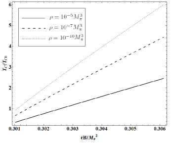
Figure 2: The critical temperature $T_{c}$ scaled with the critical temperature in the absence of a magnetic field is shown as function of the magnetic field scaled with $M_{\pi}^{2}$.

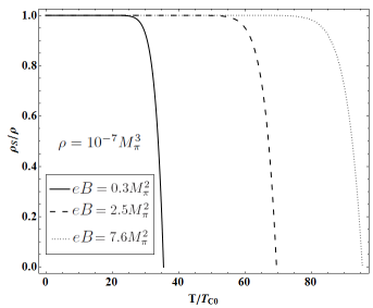
Figure 3: The superfluid charge density $\rho_{S}$ scaled with the charge density is shown as function of temperature scaled with the critical temperature $T_{c0}$. Here we use $\rho=10^{-7}M_{\pi}^{3}$.

VII Conclusions

In this article we have studied the pion condensation phenomenon in the linear sigma model keeping the isospin chemical potential close to the effective pion mass at finite temperature and in the presence of an external magnetic field. In order to find a critical temperature for the formation of the charged pion condensate, we assume a second order phase transition, looking for the minimum of the thermodynamical potential. Here we concentrate on values of the magnetic field greater than $0.3M_{\pi}^{2}$. Confirming previous results with a single charged scalar field nuestro , the magnetic field catalyzes the formation of a pion superfluid if it is strong enough.

Although the pion condensation is a different phenomenon, it is expected to be at some point related with chiral restoration Villavicencio . However, the behavior of the critical temperature in this work do not agree entirely with traditional scenario of magnetic catalysis in chiral restoration, neither with recent lattice simulations Bali:2012zg . A recent work suggest that pion condensate decreases with the magnetic field, also coinciding partially with both scenarios Kang:2013bea .

The Bose-Einstein condensation can be calculated in our case for a dilute gas but this does not mean that it should be absent for a dense gas. In fact, the assumption we have made about the second order phase transition could be relaxed, allowing also the possibility of having a first order phase transition, a crossover or even the impossibility of a superfluid state to be formed.

It is interesting to see what happen in a more complex environment, appropriate for the scenario of compact stars, when baryons and leptons at high density are included. We will discuss this problem elsewhere.

VIII Acknowledgments

The authors acknowledge support from FONDECYT under Grants No. 1130056 and No. 1120770. R.Z. acknowledges support from CONICYT under Grant No. 21110295. The authors would like to thank F. Marquez and A. Ayala for helpful discussion.

Appendix

The sum over Matsubara frequencies of Eq. (25) can be expressed in terms of the Jacobi’s theta function Jacobi

$$\sum_{n=-\infty}^{\infty}e^{-\pi xn^{2}+2\pi zn}=\frac{e^{\pi z^{2}/x}}{\sqrt{x}}\theta_{3}(-\pi z/x,e^{-\pi/x})$$

$$\quad=\frac{e^{\pi z^{2}/x}}{\sqrt{x}}\left[1+2\sum_{n=1}^{\infty}e^{-\pi n^{2}/x}\cos\left(\frac{2n\pi z}{x}\right)\right].$$ (61)

We identify $z=2i\mu sT$ and $x=4\pi T^{2}s$, and in this way the sum over Matsubara frequencies of Eq. (25) can be written as

$$\frac{1}{\beta}\sum_{n=-\infty}^{\infty}\widetilde{D}_{\pi_{\pm}}(p) = \int_{0}^{\infty}{\frac{ds}{\sqrt{\pi}}}\frac{e^{-s(m_{\pi}^{2}-\mu^{2}+p_{z}^{2}+p_{\bot}^{2}\frac{\tanh(eBs)}{eBs})}}{\cosh(eBs)}$$ (62)

$$\times \left[\frac{1}{2}+\sum_{n=1}^{\infty}e^{\frac{-n^{2}\beta^{2}}{4s}}\cosh(n\mu\beta)\right].$$

The first term inside the square bracket is independent of temperature being ultraviolet divergent and can be handled by means of dimensional regularization in the $\overline{MS}$ scheme. For the temperature dependent part, after the integration in $p_{\bot}$ and $p_{z}$, we get

$$\frac{4\lambda eB}{4\pi^{2}}\sum_{n=1}^{\infty}\cosh(\beta\mu n)\int_{0}^{\infty}{\frac{ds}{s}}\frac{e^{-sm_{B}^{2}-\beta^{2}n^{2}/(4s)}}{1-e^{-2eBs}}.$$ (63)

In the limit $T\ll m_{B}$ the integrand in Eq. (63) can be discussed in terms of the steepest descent method descent . By introducing $s\rightarrow s^{\prime}/(m_{B}T)$, the integral can be expressed as

$$I=\int{ds^{\prime}}e^{\beta m_{B}f(s^{\prime})}g(s^{\prime})\approx\frac{\sqrt{2\pi}g(s_{0})e^{\beta m_{B}f(s_{0})}}{|\beta m_{B}f^{\prime\prime}(s_{0})|^{1/2}},$$ (64)

where $f(s)=-(s+n^{2}/(4s))$ and $s_{0}=n/2$ is the saddle point. With this approximation we arrive then to equations (35), (40), (43), and (44).

References

• (1) A. Ayala, M. Loewe, J. C. Rojas and C. Villavicencio, Phys. Rev. D 86, 076006 (2012).
• (2) M. R. Schafroth, Phys. Rev.  100, 463 (1955).
• (3) R. M. May, J. Math. Phys. 6, 1462 (1965).
• (4) D. J. Toms, Phys. Rev. Lett.  69, 1152 (1992).
• (5) J. Daicic, N. E. Frankel and V. Kowalenko, Phys. Rev. Lett. 71, 1779 (1993).
• (6) D. J. Toms, Phys. Rev. D 47, 2483 (1993).
• (7) D. J. Toms, Phys. Lett. B 343, 259 (1995).
• (8) P. Elmfors, P. Liljenberg, D. Persson and B. -S. Skagerstam, Phys. Lett. B 348, 462 (1995).
• (9) A. Ayala, A. Bashir, A. Raya and A. Sanchez, Phys. Rev. D 80, 036005 (2009).
• (10) Alejandro Ayala, Luis Alberto Hernandez, Jesus Lopez, Ana Julia Mizher, Juan Cristobal Rojas, and Cristián Villavicencio, Phys. Rev. D 88 036010 (2013).
• (11) G. Baym and E. Flowers, Nucl. Phys. A 222, 29 (1974).
• (12) G. Baym and C. K. Au, Nucl. Phys. A 236, 500 (1974).
• (13) G. Baym and C. K. Au, Phys. Lett. B 51, 1 (1974).
• (14) N. K. Glendenning, Compact Stars: Nuclear Physics, Particle Physics and General Relativity (Springer-Verlag New York, Inc., second edition 2000).
• (15) See, for example, J. B. Kogut and M. A. Stephanov, The phases of quantum chromodynamics: From confinement to extreme environments,” Cambridge Monographs in Particle Physsics, Nuclear Physics and Cosmology 21, 1 (2004).
• (16) M. Loewe and C. Villavicencio, Phys. Rev. D 67, 074034 (2003); Phys. Rev. D 70, 074005 (2004); Phys. Rev. D 71, 094001 (2005).
• (17) K. Splittorff, D. Toublan and J. J. M. Verbaarschot, Nucl. Phys. B 639, 524 (2002).
• (18) D. T. Son and M. A. Stephanov, Phys. Rev. Lett 86, 592 (2001).
• (19) J. B. Kogut and D. Toublan, Phys. Rev. D 64, 034007 (2001).
• (20) Zhao Zhang and Yu-Xin Liu, Phys. Rev. C 75, 064910 (2007).
• (21) Swagato Mukherjee, Munshi G. Mustafa and Rajarshi Ray Phys. Rev. D 75, 094015 (2007).
• (22) D. Ebert and K. G. Klimenko, Eur. Phys. J. C 46, 771 (2006).
• (23) D. Ebert and K. G. Klimenko, J. Phys. G 32, 599 (2006).
• (24) K. Splittorff, D. T. Son and M. A. Stephanov, Phys. Rev. D 64, 016003 (2001).
• (25) B. Klein, D. Toublan and J. J. M. Verbaarschot, Phys. Rev. D 68, 014009 (2003).
• (26) D. Toublan and J. B. Kogut, Phys. Lett. B 564, 212 (2003).
• (27) A. Barducci, G. Pettini, L. Ravagli and R. Casalbuoni, Phys. Lett. B 564, 217 (2003).
• (28) A. Barducci, R. Casalbuoni, G. Pettini, and L. Ravagli Phys. Rev. D 69, 096004 (2004).
• (29) D. T. Son and M. A. Stephanov, Yad. Fis. 64, 899 (2001).
• (30) K. Splittdorff, D. Toublan, and J. I. M. Verbaarshot, Nucl. Phys. B 620, 290 (2002).
• (31) T. Herpay and P. Kovacs, Phys. Rev. D 78, 116008 (2008).
• (32) M. Gell-Mann and M. Levy, Nuovo Cim. 16, 705 (1960).
• (33) S. Shu and J. R. Li, J. Phys. G 31, 459 (2005).
• (34) A. J. Mizher, M. N. Chernodub and E. S. Fraga, Phys. Rev. D 82, 105016 (2010).
• (35) A. J. Mizher and E. S. Fraga, Nucl. Phys. A 831, 91 (2009).
• (36) L. He, M. Jin, and P. Zhuang, Phys. Rev. D 71, 116001 (2005).
• (37) P. E. de Brito and H. N. Nazareno, Eur. J. Phys. 28, 9 (2007).
• (38) See for example: P. A. Martin and F. Rothen, Many body problems and quantum field theory: An introduction,’ (Springer 2002)
• (39) L. Dolan and R.Jackiw, Phys. Rev. D 9 3320 (1974).
• (40) M. Le Bellac, Thermal Field Theory, (Cambridge University Press, Cambridge, 1996).
• (41) A. Das, Finite temperature field theory, (Worls Scientific, Singapore, 1997).
• (42) J. I. Kapusta, Finite-temperature field theory, (Cambridge University Press, Cambridge, 1989).
• (43) J. Schwinger, Phys. Rev. 82, 664 (1951).
• (44) B. J. Harrington and H. K. Shepard, Phys. Rev. D 16, 3437 (1977).
• (45) G. S. Bali, F. Bruckmann, G. Endrodi, Z. Fodor, S. D. Katz, S. Krieg, A. Schafer and K.K. Szabo, JHEP 1202, 044 (2012);
G. S. Bali, F. Bruckmann, G. Endrodi, Z. Fodor, S. D. Katz and A. Schafer, Phys. Rev. D 86, 071502 (2012)
• (46) X. Kang, M. Jin, J. Xiong and J. Li, arXiv:1310.3012 [hep-ph].
• (47) See, for example: N. Temme, Special Functions: An Introduction to the Classical Functions of Mathematical Physics, (Wiley-Interscience 1992).
• (48) George B. Arfken, Hans J. Weber and Frank E. Harris, Mathematical Methods for Physicists, (Academic Press; 6th edition, 2005).