ROP: Matrix recovery via rank-one projections

Abstract

Estimation of low-rank matrices is of significant interest in a range of contemporary applications. In this paper, we introduce a rank-one projection model for low-rank matrix recovery and propose a constrained nuclear norm minimization method for stable recovery of low-rank matrices in the noisy case. The procedure is adaptive to the rank and robust against small perturbations. Both upper and lower bounds for the estimation accuracy under the Frobenius norm loss are obtained. The proposed estimator is shown to be rate-optimal under certain conditions. The estimator is easy to implement via convex programming and performs well numerically.

The techniques and main results developed in the paper also have implications to other related statistical problems. An application to estimation of spiked covariance matrices from one-dimensional random projections is considered. The results demonstrate that it is still possible to accurately estimate the covariance matrix of a high-dimensional distribution based only on one-dimensional projections.

FLA

and T1Supported in part by NSF FRG Grant DMS-08-54973, NSF Grant DMS-12-08982 and NIH Grant R01 CA127334-05.

1 Introduction

Accurate recovery of low-rank matrices has a wide range of applications, including quantum state tomography Alquier , Gross , face recognition Basri , Candes-Li , recommender systems Koren and linear system identification and control RechtMatrix . For example, a key step in reconstructing the quantum states in low-rank quantum tomography is the estimation of a low-rank matrix based on Pauli measurements Gross , Wang . And phase retrieval, a problem which arises in a range of signal and image processing applications including X-ray crystallography, astronomical imaging and diffraction imaging, can be reformulated as a low-rank matrix recovery problem CandesRIPfail , Candes-Li . See Recht et al. RechtMatrix and Candès and Plan CandesOracle for further references and discussions.

Motivated by these applications, low-rank matrix estimation based on a small number of measurements has drawn much recent attention in several fields, including statistics, electrical engineering, applied mathematics and computer science. For example, Candès and Recht CandesRecht , Candès and Tao CandesTao and Recht RechtImproved considered the exact recovery of a low-rank matrix based on a subset of uniformly sampled entries. Negahban and Wainwright Negahban investigated matrix completion under a row/column weighted random sampling scheme. Recht et al. RechtMatrix , Candès and Plan CandesOracle and Cai and Zhang CaiZhang , CaiZhang2 , CaiZhang3 studied matrix recovery based on a small number of linear measurements in the framework of Restricted Isometry Property (RIP), and Koltchinskii et al. KLT proposed the penalized nuclear norm minimization method and derived a general sharp oracle inequality under the condition of restrict isometry in expectation.

The basic model for low-rank matrix recovery can be written as

$$y=\mathcal{X}(A)+z,$$ (1)

where $\mathcal{X}\dvtx\mathbb{R}^{p_{1}\times p_{2}}\to\mathbb{R}^{n}$ is a linear map, $A\in\mathbb{R}^{p_{1}\times p_{2}}$ is an unknown low-rank matrix and $z$ is a noise vector. The goal is to recover the low-rank matrix $A$ based on the measurements $(\mathcal{X},y)$. The linear map $\mathcal{X}$ can be equivalently specified by $n$ $p_{1}\times p_{2}$ measurement matrices $X_{1},\ldots,X_{n}$ with

$$\mathcal{X}(A)=\bigl{(}\langle X_{1},A\rangle,\langle X_{2},A\rangle,\ldots,\langle X_{n},A\rangle\bigr{)}^{\intercal},$$ (2)

where the inner product of two matrices of the same dimensions is defined as $\langle X,Y\rangle=\sum_{i,j}X_{ij}Y_{ij}$. Since $\langle X,Y\rangle=\operatorname{trace}(X^{\intercal}Y)$, (1) is also known as trace regression.

A common approach to low-rank matrix recovery is the constrained nuclear norm minimization method which estimates $A$ by

$$\hat{A}=\mathop{\arg\min}_{M}\bigl{\{}\|M\|_{\ast}\dvtx y-\mathcal{X}(M)\in\mathcal{Z}\bigr{\}}.$$ (3)

Here, $\|X\|_{\ast}$ is the nuclear norm of the matrix $X$ which is defined to be the sum of its singular values, and $\mathcal{Z}$ is a bounded set determined by the noise structure. For example, $\mathcal{Z}=\{0\}$ in the noiseless case and $\mathcal{Z}$ is the feasible set of the error vector $z$ in the case of bounded noise. This constrained nuclear norm minimization method has been well studied. See, for example, RechtMatrix , CandesOracle , Oymak , CaiZhang , CaiZhang2 , CaiZhang3 .

Two random design models for low-rank matrix recovery have been particularly well studied in the literature. One is the so-called “Gaussian ensemble” RechtMatrix , CandesOracle , where the measurement matrices $X_{1},\ldots,X_{n}$ are random matrices with i.i.d. Gaussian entries. By exploiting the low-dimensional structure, the number of linear measurements can be far smaller than the number of entries in the matrix to ensure stable recovery. It has been shown that a matrix $A$ of rank $r$ can be stably recovered by nuclear norm minimization with high probability, provided that $n\gtrsim r(p_{1}+p_{2})$ CandesOracle . One major disadvantage of the Gaussian ensemble design is that it requires $O(np_{1}p_{2})$ bytes of storage space for $\mathcal{X}$, which can be excessively large for the recovery of large matrices. For example, at least $45$ TB of space is need to store the measurement matrices $M_{i}$ in order to ensure accurate reconstruction of 10,000${}\times{}$10,000 matrices of rank 10. (See more discussion in Section 5.) Another popular design is the “matrix completion” model CandesRecht , CandesTao , RechtImproved , under which the individual entries of the matrix $A$ are observed at randomly selected positions. In terms of the measurement matrices $X_{i}$ in (2), this can be interpreted as

$$\mathcal{X}(A)=\bigl{(}\bigl{\langle}e_{i_{1}}e_{j_{1}}^{\intercal},A\bigr{\rangle},\bigl{\langle}e_{i_{2}}e_{j_{2}}^{\intercal},A\bigr{\rangle},\ldots,\bigl{\langle}e_{i_{n}}e_{j_{n}}^{\intercal},A\bigr{\rangle}\bigr{)}^{\intercal},$$ (4)

where $e_{i}=(0,\ldots,0,\overbrace{1}^{i{\mathrm{th}}},0,\ldots,0)$ is the $i$th standard basis vector, and $i_{1},\ldots,\break i_{n}$ and $j_{1},\ldots,j_{n}$ are randomly and uniformly drawn with replacement from $\{1,\ldots,p_{1}\}$ and $\{1,\ldots,p_{2}\}$, respectively. However, as pointed out in CandesRecht , RechtImproved , additional structural assumptions, which are not intuitive and difficult to check, on the unknown matrix $A$ are needed in order to ensure stable recovery under the matrix completion model. For example, it is impossible to recover spiked matrices under the matrix completion model. This can be easily seen from a simple example where the matrix $A$ has only one nonzero row. In this case, although the matrix is only of rank one, it is not recoverable under the matrix completion model unless all the elements on the nonzero row are observed.

In this paper, we introduce a “Rank-One Projection” (ROP) model for low-rank matrix recovery and propose a constrained nuclear norm minimization method for this model. Under the ROP model, we observe

$$y_{i}=\bigl{(}\beta^{(i)}\bigr{)}^{\intercal}A\gamma^{(i)}+z_{i},\qquad i=1,\ldots,n,$$ (5)

where $\beta^{(i)}$ and $\gamma^{(i)}$ are random vectors with entries independently drawn from some distribution $\mathcal{P}$, and $z_{i}$ are random errors. In terms of the linear map $\mathcal{X}\dvtx\mathbb{R}^{p_{1}\times p_{2}}\to\mathbb{R}^{n}$ in (1), it can be defined as

$$\bigl{[}\mathcal{X}(A)\bigr{]}_{i}=\bigl{(}\beta^{(i)}\bigr{)}^{\intercal}A\gamma^{(i)},\qquad i=1,\ldots,n.$$ (6)

Since the measurement matrices $X_{i}=\beta^{(i)}(\gamma^{(i)})^{\intercal}$ are of rank-one, we call the model (5) a “Rank-One Projection” (ROP) model. It is easy to see that the storage for the measurement vectors in the ROP model (5) is $O(n(p_{1}+p_{2}))$ bytes which is significantly smaller than $O(np_{1}p_{2})$ bytes required for the Gaussian ensemble.

We first establish a sufficient identifiability condition in Section 2 by considering the problem of exact recovery of low-rank matrices in the noiseless case. It is shown that, with high probability, ROP with $n\gtrsim r(p_{1}+p_{2})$ random projections is sufficient to ensure exact recovery of all rank-$r$ matrices through the constrained nuclear norm minimization. The required number of measurements $O(r(p_{1}+p_{2}))$ is rate optimal for any linear measurement model since a rank-$r$ matrix $A\in\mathbb{R}^{p_{1}+p_{2}}$ has the degree of freedom $r(p_{1}+p_{2}-r)$. The Gaussian noise case is of particular interest in statistics. We propose a new constrained nuclear norm minimization estimator and investigate its theoretical and numerical properties in the Gaussian noise case. Both upper and lower bounds for the estimation accuracy under the Frobenius norm loss are obtained. The estimator is shown to be rate-optimal when the number of rank-one projections satisfies either $n\gtrsim(p_{1}+p_{2})\log(p_{1}+p_{2})$ or $n\sim r(p_{1}+p_{2})$. The lower bound also shows that if the number of measurements $n<r\max(p_{1},p_{2})$, then no estimator can recover rank-$r$ matrices consistently. The general case where the matrix $A$ is only approximately low-rank is also considered. The results show that the proposed estimator is adaptive to the rank $r$ and robust against small perturbations. Extensions to the sub-Gaussian design and sub-Gaussian noise distribution are also considered.

The ROP model can be further simplified by taking $\beta^{(i)}=\gamma^{(i)}$ if the low-rank matrix $A$ is known to be symmetric. This is the case in many applications, including low-dimensional Euclidean embedding Trosset , RechtMatrix , phase retrieval CandesRIPfail , Candes-Li and covariance matrix estimation Chen , CaiMaWu1 , CaiMaWu2 . In such a setting, the ROP design can be simplified to Symmetric Rank-One Projections (SROP)

$$\bigl{[}\mathcal{X}(A)\bigr{]}_{i}=\bigl{(}\beta^{(i)}\bigr{)}^{\intercal}A\beta^{(i)}.$$

We will show that the results for the general ROP model continue to hold for the SROP model when $A$ is known to be symmetric. Recovery of symmetric positive definite matrices in the noiseless and $\ell_{1}$-bounded noise settings has also been considered in a recent paper by Chen et al. Chen which was posted on arXiv at the time of the writing of the present paper. Their results and techniques for symmetric positive definite matrices are not applicable to the recovery of general low-rank matrices. See Section 6 for more discussions.

The techniques and main results developed in the paper also have implications to other related statistical problems. In particular, the results imply that it is possible to accurately estimate a spiked covariance matrix based only on one-dimensional projections. Spiked covariance matrix model has been well studied in the context of Principal Component Analysis (PCA) based on i.i.d. data where one observes $p$-dimensional vectors $X^{(1)},\ldots,X^{(n)}\stackrel{{\scriptstyle\mathrm{i.i.d.}}}{{\sim}}N(0,\Sigma)$ with $\Sigma=I_{p}+\Sigma_{0}$ and $\Sigma_{0}$ being low-rank Johnstone , Birnbaum , CaiMaWu1 , CaiMaWu2 . This covariance structure and its variations have been used in many applications including signal processing, financial econometrics, chemometrics and population genetics. See, for example, Fan , Nadler , Patterson , Price , Wax . Suppose that the random vectors $X^{(1)},\ldots,X^{(n)}$ are not directly observable. Instead, we observe only one-dimensional random projections of $X^{(i)}$,

$$\xi_{i}=\bigl{\langle}\beta^{(i)},X^{(i)}\bigr{\rangle},\qquad i=1,\ldots,n,$$

where $\beta^{(i)}\stackrel{{\scriptstyle\mathrm{i.i.d.}}}{{\sim}}N(0,I_{p})$. It is somewhat surprising that it is still possible to accurately estimate the spiked covariance matrix $\Sigma$ based only on the one-dimensional projections $\{\xi_{i}\dvtx i=1,\ldots,n\}$. This covariance matrix recovery problem is also related to the recent literature on covariance sketching Nowak1 , Nowak2 , which aims to recover a symmetric matrix $A$ (or a general rectangular matrix $B$) from low-dimensional projections of the form $X^{\intercal}AX$ (or $X^{\intercal}BY$). See Section 4 for further discussions.

The proposed methods can be efficiently implemented via convex programming. A simulation study is carried out to investigate the numerical performance of the proposed nuclear norm minimization estimators. The numerical results indicate that ROP with $n\geq 5r\max(p_{1},p_{2})$ random projections is sufficient to ensure the exact recovery of rank-$r$ matrices through constrained nuclear norm minimization and show that the procedure is robust against small perturbations, which confirm the theoretical results developed in the paper. The proposed estimator outperforms two other alternative procedures numerically in the noisy case. In addition, the proposed method is illustrated through an image compression example.

The rest of the paper is organized as follows. In Section 2, after introducing basic notation and definitions, we consider exact recovery of low-rank matrices in the noiseless case and establish a sufficient identifiability condition. A constrained nuclear norm minimization estimator is introduced for the Gaussian noise case. Both upper and lower bounds are obtained for estimation under the Frobenius norm loss. Section 3 considers extensions to sub-Gaussian design and sub-Gaussian noise distributions. An application to estimation of spiked covariance matrices based on one-dimensional projections is discussed in detail in Section 4. Section 5 investigates the numerical performance of the proposed procedure through a simulation study and an image compression example. A brief discussion is given in Section 6. The main results are proved in Section 7 and the proofs of some technical lemmas are given in the supplementary material Supplement .

2 Matrix recovery under Gaussian noise

In this section, we first establish an identifiability condition for the ROP model by considering exact recovery in the noiseless case, and then focus on low-rank matrix recovery in the Gaussian noise case.

We begin with the basic notation and definitions. For a vector $\beta\in\mathbb{R}^{n}$, we use $\|\beta\|_{q}=\sqrt[q]{\sum_{i=1}^{n}|\beta_{i}|^{q}}$ to define its vector $q$-norm. For a matrix $X\in\mathbb{R}^{p_{1}\times p_{2}}$, the Frobenius norm is $\|X\|_{F}=\sqrt{\sum_{i=1}^{p_{1}}\sum_{j=1}^{p_{2}}X_{ij}^{2}}$ and the spectral norm $\|\cdot\|$ is $\|X\|=\sup_{\|\beta\|_{2}\leq 1}\|X\beta\|_{2}$. For a linear map $\mathcal{X}=(X_{1},\ldots,X_{n})$ from $\mathbb{R}^{p_{1}\times p_{2}}$ to $\mathbb{R}^{n}$ given by (2), its dual operator $\mathcal{X}^{\ast}\dvtx\mathbb{R}^{n}\to\mathbb{R}^{p_{1}\times p_{2}}$ is defined as $\mathcal{X}^{\ast}(z)=\sum_{i=1}^{n}z_{i}X_{i}$. For a matrix $X\in\mathbb{R}^{p_{1}\times p_{2}}$, let $X=\sum_{i}a_{i}u_{i}v_{i}^{\intercal}$ be the singular value decomposition of $X$ with the singular values $a_{1}\geq a_{2}\geq\cdots\geq 0$. We define $X_{\max(r)}=\sum_{i=1}^{r}a_{i}u_{i}v_{i}^{\intercal}$ and $X_{-\max(r)}=X-X_{\max(r)}=\sum_{i\geq r+1}a_{i}u_{i}v_{i}^{\intercal}$. For any two sequences $\{a_{n}\}$ and $\{b_{n}\}$ of positive numbers, denote by $a_{n}\gtrsim b_{n}$ when $a_{n}\geq Cb_{n}$ for some uniform constant $C$ and denote by $a_{n}\sim b_{n}$ if $a_{n}\gtrsim b_{n}$ and $b_{n}\gtrsim a_{n}$.

We use the phrase “rank-$r$ matrices” to refer to matrices of rank at most $r$ and denote by $\mathbb{S}^{p}$ the set of all $p\times p$ symmetric matrices. A linear map $\mathcal{X}\dvtx\mathbb{R}^{p_{1}\times p_{2}}\to\mathbb{R}^{n}$ is called ROP from distribution $\mathcal{P}$ if $\mathcal{X}$ is defined as in (6) with all the entries of $\beta^{(i)}$ and $\gamma^{(i)}$ independently drawn from the distribution $\mathcal{P}$.

2.1 RUB, identifiability, and exact recovery in the noiseless case

An important step toward understanding the constrained nuclear norm minimization is the study of exact recovery of low-rank matrices in the noiseless case which also leads to a sufficient identifiability condition. A widely used framework in the low-rank matrix recovery literature is the Restricted Isometry Property (RIP) in the matrix setting. See RechtMatrix , CandesOracle , Rohde , CaiZhang , CaiZhang2 , CaiZhang3 . However, the RIP framework is not well suited for the ROP model and would lead to suboptimal results. See Section 2.2 for more discussions on the RIP and other conditions used in the literature. See also CandesRIPfail . In this section, we introduce a Restricted Uniform Boundedness (RUB) condition which will be shown to guarantee the exact recovery of low-rank matrices in the noiseless case and stable recovery in the noisy case through the constrained nuclear norm minimization. It will also be shown that the RUB condition are satisfied by a range of random linear maps with high probability.

Definition 2.1 ((Restricted Uniform Boundedness)).

For a linear map $\mathcal{X}\dvtx\mathbb{R}^{p_{1}\times p_{2}}\to\mathbb{R}^{n}$, if there exist uniform constants $C_{1}$ and $C_{2}$ such that for all nonzero rank-$r$ matrices $A\in\mathbb{R}^{p_{1}\times p_{2}}$

$$C_{1}\leq{\|\mathcal{X}(A)\|_{1}/n\over\|A\|_{F}}\leq C_{2},$$

where $\|\cdot\|_{1}$ means the vector $\ell_{1}$ norm, then we say that $\mathcal{X}$ satisfies the Restricted Uniform Boundedness (RUB) condition of order $r$ and constants $C_{1}$ and $C_{2}$.

In the noiseless case, we observe $y=\mathcal{X}(A)$ and estimate the matrix $A$ through the constrained nuclear norm minimization

$$A_{\ast}=\mathop{\arg\min}_{M}\bigl{\{}\|M\|_{\ast}\dvtx\mathcal{X}(M)=y\bigr{\}}.$$ (7)

The following theorem shows that the RUB condition guarantees the exact recovery of all rank-$r$ matrices.

Theorem 2.1.

Let $k\geq 2$ be an integer. Suppose $\mathcal{X}$ satisfies RUB of order $kr$ with $C_{2}/C_{1}<\sqrt{k}$, then the nuclear norm minimization method recovers all rank-$r$ matrices. That is, for all rank-$r$ matrices $A$ and $y=\mathcal{X}(A)$, we have $A_{\ast}=A$, where $A_{\ast}$ is given by (7).

Theorem 2.1 shows that RUB of order $kr$ with $C_{2}/C_{1}<\sqrt{k}$ is a sufficient identifiability condition for the low-rank matrix recovery model (1) in the noisy case. The following result shows that the RUB condition is satisfied with high probability under the ROP model with a sufficient number of measurements.

Theorem 2.2.

Suppose $\mathcal{X}\dvtx\mathbb{R}^{p_{1}\times p_{2}}\to\mathbb{R}^{n}$ is ROP from the standard normal distribution. For integer $k\geq 2$, positive numbers $C_{1}<\frac{1}{3}$ and $C_{2}>1$, there exist constants $C$ and $\delta$, not depending on $p_{1},p_{2}$ and $r$, such that if

$$n\geq Cr(p_{1}+p_{2}),$$ (8)

then with probability at least $1-e^{-n\delta}$, $\mathcal{X}$ satisfies RUB of order $kr$ and constants $C_{1}$ and $C_{2}$.

Remark 2.1.

The condition $n\geq O(r(p_{1}+p_{2}))$ on the number of measurements is indeed necessary for $\mathcal{X}$ to satisfy nontrivial RUB with $C_{1}>0$. Note that the degree of freedom of all rank-$r$ matrices of $\mathbb{R}^{p_{1}\times p_{2}}$ is $r(p_{1}+p_{2}-r)\geq\frac{1}{2}r(p_{1}+p_{2})$. If $n<\frac{1}{2}r(p_{1}+p_{2})$, there must exist a nonzero rank-$r$ matrix $A\in\mathbb{R}^{p_{1}\times p_{2}}$ such that $\mathcal{X}(A)=0$, which leads to the failure of any nontrivial RUB for $\mathcal{X}$.

As a direct consequence of Theorems 2.1 and 2.2, ROP with the number of measurements $n\geq Cr(p_{1}+p_{2})$ guarantees the exact recovery of all rank-$r$ matrices with high probability.

Corollary 2.1.

Suppose $\mathcal{X}\dvtx\mathbb{R}^{p_{1}\times p_{2}}\to\mathbb{R}^{n}$ is ROP from the standard normal distribution. There exist uniform constants $C$ and $\delta$ such that, whenever $n\geq Cr(p_{1}+p_{2})$, the nuclear norm minimization estimator $A_{*}$ given in (7) recovers all rank-$r$ matrices $A\in\mathbb{R}^{p_{1}\times p_{2}}$ exactly with probability at least $1-e^{-n\delta}$.

Note that the required number of measurements $O(r(p_{1}+p_{2}))$ above is rate optimal, since the degree of freedom for a matrix $A\in\mathbb{R}^{p_{1}+p_{2}}$ of rank $r$ is $r(p_{1}+p_{2}-r)$, and thus at least $r(p_{1}+p_{2}-r)$ measurements are needed in order to recover $A$ exactly using any method.

2.2 RUB, RIP and other conditions

We have shown that RUB implies exact recovery in the noiseless and proved that the random rank-one projections satisfy RUB with high probability whenever the number of measurements $n\geq Cr(p_{1}+p_{2})$. As mentioned earlier, other conditions, including the Restricted Isometry Property (RIP), RIP in expectation and Spherical Section Property (SSP), have been introduced for low-rank matrix recovery based on linear measurements. Among them, RIP is perhaps the most widely used. A linear map $\mathcal{X}\dvtx\mathbb{R}^{p_{1}\times p_{2}}\to\mathbb{R}^{n}$ is said to satisfy RIP of order $r$ with positive constants $C_{1}$ and $C_{2}$ if

$$C_{1}\leq\frac{\|\mathcal{X}(A)\|_{2}/\sqrt{n}}{\|A\|_{F}}\leq C_{2}$$

for all rank-$r$ matrices $A$. Many results have been given for low-rank matrices under the RIP framework. For example, Recht et al. RechtMatrix showed that Gaussian ensembles satisfy RIP with high probability under certain conditions on the dimensions. Candès and Plan CandesOracle provided a lower bound and oracle inequality under the RIP condition. Cai and Zhang CaiZhang , CaiZhang2 , CaiZhang3 established the sharp bounds for the RIP conditions that guarantee accurate recovery of low-rank matrices.

However, the RIP framework is not suitable for the ROP model considered in the present paper. The following lemma is proved in the supplementary material Supplement .

Lemma 2.1.

Suppose $\mathcal{X}\dvtx\mathbb{R}^{p_{1}\times p_{2}}\to\mathbb{R}^{n}$ is ROP from the standard normal distribution. Let

$$C_{1}=\min_{A\dvtx\operatorname{rank}(A)=1}\frac{\|\mathcal{X}(A)\|_{2}/\sqrt{n}}{\|A\|_{F}}\quad\mbox{and}\quad C_{2}=\max_{A\dvtx\operatorname{rank}(A)=1}\frac{\|\mathcal{X}(A)\|_{2}/\sqrt{n}}{\|A\|_{F}}.$$

Then for all $t>1$, $C_{2}/C_{1}\geq\sqrt{p_{1}p_{2}/(4tn)}$ with probability at least $1-e^{-p_{1}/4}-e^{-p_{2}/4}-\frac{8}{n(t-1)^{2}}$.

Lemma 2.1 implies that at least $O(p_{1}p_{2})$ number of measurements are needed in order to ensure that $\mathcal{X}$ satisfies the RIP condition that guarantees the recovery of only rank-one matrices. Since $O(p_{1}p_{2})$ is the degree of freedom for all matrices $A\in\mathbb{R}^{p_{1}\times p_{2}}$ and it is the number of measurements needed to recover all $p_{1}\times p_{2}$ matrices (not just the low-rank matrices), Lemma 2.1 shows that the RIP framework is not suitable for the ROP model. In comparison, Theorem 2.2 shows that if $n\geq O(r(p_{1}+p_{2}))$, then with high probability $\mathcal{X}$ satisfies the RUB condition of order $r$ with bounded $C_{2}/C_{1}$, which ensures the exact recovery of all rank-$r$ matrices.

The main technical reason for the failure of RIP under the ROP model is that RIP requires an upper bound for

$$\max_{A\in\mathcal{C}}\bigl{\|}\mathcal{X}(A)\bigr{\|}_{2}^{2}/n=\max_{A\in\mathcal{C}}\Biggl{(}\sum_{j=1}^{n}\bigl{(}\bigl{(}\beta^{(j)}\bigr{)}^{\intercal}A\gamma^{(j)}\bigr{)}^{2}\Biggr{)}\Big{/}n,$$ (9)

where $\mathcal{C}$ is a set containing low-rank matrices. The right-hand side of (9) involves the 4th power of the Gaussian (or sub-Gaussian) variables $\beta^{(j)}$ and $\gamma^{(j)}$. A much larger $n$ than the bound given in (8) is needed in order for the linear map $\mathcal{X}$ to satisfy the required RIP condition, which would lead to suboptimal result.

Koltchinskii et al. KLT uses RIP in expectation, which is a weaker condition than RIP. A random linear map $\mathcal{X}\dvtx\mathbb{R}^{p_{1}\times p_{2}}\to\mathbb{R}^{n}$ is said to satisfy RIP in expectation of order $r$ with parameters $0<\mu<\infty$ and $0\leq\delta_{r}<1$ if

$$(1-\delta_{r})\|A\|_{F}^{2}\leq\mu\frac{1}{n}E\bigl{\|}\mathcal{X}(A)\bigr{\|}_{2}^{2}\leq(1+\delta_{r})\|A\|_{F}^{2}$$

for all rank-$r$ matrices $A\in\mathbb{R}^{p_{1}\times p_{2}}$. This condition was originally introduced by Koltchinskii et al. KLT to prove an oracle inequality for the estimator they proposed and a minimax lower bound. The condition is not sufficiently strong to guarantee the exact recovery of rank-$r$ matrices in the noiseless case. To be more specific, the bounds in Theorems 1 and 2 in KLT depend on ${\mathbf{M}}=\|\frac{1}{n}\sum_{i=1}^{n}(y_{i}X_{i}-E(y_{i}X_{i}))\|$, which might be nonzero even in the noiseless case. In fact, in the ROP model considered in the present paper, we have

$$\frac{1}{n}E\|\mathcal{X}\|_{2}^{2} = \frac{1}{n}\sum_{i=1}^{n}E\bigl{(}\beta^{(i)T}A\gamma^{(i)}\bigr{)}^{2}=E\bigl{(}\beta^{\intercal}A\gamma\gamma^{\intercal}A^{\intercal}\beta\bigr{)}$$

$$= E\operatorname{tr}\bigl{(}A\gamma\gamma^{\intercal}A^{\intercal}\beta\beta^{\intercal}\bigr{)}=\operatorname{tr}\bigl{(}AA^{\intercal}\bigr{)}=\|A\|_{F}^{2}$$

which means RIP in expectation is met for $\mu=1$ and $\delta_{r}=0$ for any number of measurements $n$. However, as we discussed earlier in this section that at least $O(r(p_{1}+p_{2}))$ measurements are needed to guarantee the model identifiability for recovery of all rank-$r$ matrices, we can see that RIP in expectation cannot ensure recovery.

Dvijotham and Fazel Dvijotham and Oymak et al. Oymak11 used a condition called the Spherical Section Property (SSP) which focuses on the null space of $\mathcal{X}$. $\operatorname{Null}(\mathcal{X})$ is said to satisfy $\Delta$-SSP if for all $Z\in\operatorname{Null}(\mathcal{X})\setminus\{0\}$, $\|Z\|_{\ast}/\|Z\|_{F}\geq\sqrt{\Delta}$. Dvijotham and Fazel Dvijotham showed that if $\mathcal{X}$ satisfies $\Delta$-SSP, $p_{1}\leq p_{2}$ and $\operatorname{rank}(A)<\min(3p_{1}/4-\sqrt{9p_{1}^{2}/16-p_{1}\Delta/4},p_{1}/2)$, the nuclear norm minimization (7) recovers $A$ exactly in the noiseless case. However, the SSP condition is difficult to utilize in the ROP framework since it is hard to characterize the matrices $Z\in\operatorname{Null}(\mathcal{X})$ when $\mathcal{X}$ is rank-one projections.

2.3 Gaussian noise case

We now turn to the Gaussian noise case where $z_{i}\stackrel{{\scriptstyle\mathrm{i.i.d.}}}{{\sim}}N(0,\sigma^{2})$ in (5). We begin by introducing a constrained nuclear norm minimization estimator. Define two sets

$$\mathcal{Z}_{1}=\bigl{\{}z\dvtx\|z\|_{1}/n\leq\sigma\bigr{\}}\quad\mbox{and}\quad\mathcal{Z}_{2}=\bigl{\{}z\dvtx\bigl{\|}\mathcal{X}^{\ast}(z)\bigr{\|}\leq\eta\bigr{\}},$$ (10)

where $\eta=\sigma(12\sqrt{\log n}(p_{1}+p_{2})+6\sqrt{2n(p_{1}+p_{2})})$, and let

$$\mathcal{Z}_{G}=\mathcal{Z}_{1}\cap\mathcal{Z}_{2}.$$ (11)

Note that both $\mathcal{Z}_{1}$ and $\mathcal{Z}_{2}$ are convex sets and so is $\mathcal{Z}_{G}$. Our estimator of $A$ is given by

$$\hat{A}=\mathop{\arg\min}_{M}\bigl{\{}\|M\|_{\ast}\dvtx y-\mathcal{X}(M)\in\mathcal{Z}_{G}\bigr{\}}.$$ (12)

The following theorem gives the rate of convergence for the estimator $\hat{A}$ under the squared Frobenius norm loss.

Theorem 2.3 ((Upper bound)).

Let $\mathcal{X}$ be ROP from the standard normal distribution and let $z_{1},\ldots,z_{n}\stackrel{{\scriptstyle\mathit{i.i.d.}}}{{\sim}}N(0,\sigma^{2})$. Then there exist uniform constants $C$, $W$ and $\delta$ such that, whenever $n\geq Cr(p_{1}+p_{2})$, the estimator $\hat{A}$ given in (12) satisfies

$$\|\hat{A}-A\|_{F}^{2}\leq W\sigma^{2}\min\biggl{(}\frac{r\log n(p_{1}+p_{2})^{2}}{n^{2}}+\frac{r(p_{1}+p_{2})}{n},1\biggr{)}$$ (13)

for all rank-$r$ matrices $A$, with probability at least $1-11/n-3\exp(-\delta(p_{1}+p_{2}))$.

Moreover, we have the following lower bound result for ROP.

Theorem 2.4 ((Lower bound)).

Assume that $\mathcal{X}$ is ROP from the standard normal distribution and that $z_{1},\ldots,z_{n}\stackrel{{\scriptstyle\mathit{i.i.d.}}}{{\sim}}N(0,\sigma^{2})$. There exists a uniform constant $C$ such that, when $n>Cr\max(p_{1},p_{2})$, with probability at least $1-26n^{-1}$,

$$\inf_{\hat{A}}\sup_{A\in\mathbb{R}^{p_{1}\times p_{2}}\dvtx\operatorname{rank}(A)=r}P_{z}\biggl{(}\|\hat{A}-A\|_{F}^{2}\geq\frac{\sigma^{2}r(p_{1}+p_{2})}{32n}\biggr{)}$$

(14)

$$\qquad\geq 1-e^{-(p_{1}+p_{2})r/64},$$

$$\inf_{\hat{A}}\sup_{A\in\mathbb{R}^{p_{1}\times p_{2}}\dvtx\operatorname{rank}(A)=r}E_{z}\|\hat{A}-A\|_{F}^{2}\geq\frac{\sigma^{2}r(p_{1}+p_{2})}{4n},$$ (15)

where $E_{z}$, and $P_{z}$ are the expectation and probability with respect to the distribution of $z$.

When $n<r\max(p_{1},p_{2})$, then

$$\inf_{\hat{A}}\sup_{A\in\mathbb{R}^{p_{1}\times p_{2}}\dvtx\operatorname{rank}(A)=r}E_{z}\|\hat{A}-A\|_{F}^{2}=\infty.$$ (16)

Comparing Theorems 2.3 and 2.4, our proposed estimator is rate optimal in the Gaussian noise case when $n\gtrsim\log n(p_{1}+p_{2})$ [which is equivalent to $n\gtrsim(p_{1}+p_{2})\log(p_{1}+p_{2})$] or $n\sim r(p_{1}+p_{2})$. Since $n\gtrsim r(p_{1}+p_{2})$, this condition is also implied by $r\gtrsim\log(p_{1}+p_{2})$. Theorem 2.4 also shows that no method can recover matrices of rank $r$ consistently if the number of measurements $n$ is smaller than $r\max(p_{1},p_{2})$.

The result in Theorem 2.3 can also be extended to the more general case where the matrix of interest $A$ is only approximately low-rank. Let $A=A_{\max(r)}+A_{-\max(r)}$.

Proposition 2.1.

Under the assumptions of Theorem 2.3, there exist uniform constants $C$, $W_{1}$, $W_{2}$ and $\delta$ such that, whenever $n\geq Cr(p_{1}+p_{2})$, the estimator $\hat{A}$ given in (12) satisfies

$$\|\hat{A}-A\|_{F}^{2} \leq W_{1}\sigma^{2}\min\biggl{(}\frac{r\log n(p_{1}+p_{2})^{2}}{n^{2}}+\frac{r(p_{1}+p_{2})}{n},1\biggr{)}$$

$${}+W_{2}\frac{\|A_{-\max(r)}\|_{\ast}^{2}}{r}$$

for all matrices $A\in\mathbb{R}^{p_{1}\times p_{2}}$, with probability at least $1-11/n-3\exp(-\delta(p_{1}+p_{2}))$.

If the matrix $A$ is approximately of rank $r$, then $\|A_{-\max(r)}\|_{\ast}$ is small, and the estimator $\hat{A}$ continues to perform well. This result shows that the constrained nuclear norm minimization estimator is adaptive to the rank $r$ and robust against perturbations of small amplitude.

Remark 2.2.

All the results remain true if the Gaussian design is replaced by the Rademacher design where entries of $\beta^{(i)}$ and $\gamma^{(i)}$ are i.i.d. $\pm 1$ with probability ${1\over 2}$. More general sub-Gaussian design case will be discussed in Section 3.

Remark 2.3.

The estimator $\hat{A}$ we propose here is the minimizer of the nuclear norm under the constraint of the intersection of two convex sets $\mathcal{Z}_{1}$ and $\mathcal{Z}_{2}$. Nuclear norm minimization under either one of the two constraints, called “$\ell_{1}$ constraint nuclear norm minimization” ($\mathcal{Z}=\mathcal{Z}_{1}$) and “matrix Dantzig Selector” ($\mathcal{Z}=\mathcal{Z}_{2}$), has been studied before in various settings CandesOracle , RechtMatrix , CaiZhang , CaiZhang2 , CaiZhang3 , Chen . Our analysis indicates the following: [3.]

The $\ell_{1}$ constraint minimization performs better than the matrix Dantzig Selector for small $n$ ($n\sim r(p_{1}+p_{2})$) when $r\ll\log n$.

The matrix Dantzig Selector outperforms the $\ell_{1}$ constraint minimization for large $n$ as the loss of the matrix Dantzig Selector decays at the rate $O(n^{-1})$.

The proposed estimator $\hat{A}$ combines the advantages of the two estimators. See Section 5 for a comparison of numerical performances of the three methods.

2.4 Recovery of symmetric matrices

For applications such as low-dimensional Euclidean embedding Trosset , RechtMatrix , phase retrieval CandesRIPfail , Candes-Li and covariance matrix estimation Chen , CaiMaWu1 , CaiMaWu2 , the low-rank matrix $A$ of interest is known to be symmetric. Examples of such matrices include distance matrices, Gram matrices, and covariance matrices. When the matrix $A$ is known to be symmetric, the ROP design can be further simplified by taking $\beta^{(i)}=\gamma^{(i)}$.

Denote by $\mathbb{S}^{p}$ the set of all $p\times p$ symmetric matrices in $\mathbb{R}^{p\times p}$. Let $\beta^{(1)}$, $\beta^{(2)},\ldots,\beta^{(n)}$ be independent $p$-dimensional random vectors with i.i.d. entries generated from some distribution $\mathcal{P}$. Define a linear map $\mathcal{X}\dvtx\mathbb{S}^{p}\to\mathbb{R}^{n}$ by

$$\bigl{[}\mathcal{X}(A)\bigr{]}_{i}=\bigl{(}\beta^{(i)}\bigr{)}^{\intercal}A\beta^{(i)},\qquad i=1,\ldots,n.$$

We call such a linear map $\mathcal{X}$ “Symmetric Rank-One Projections” (SROP) from the distribution $\mathcal{P}$.

Suppose we observe

$$y_{i}=\bigl{(}\beta^{(i)}\bigr{)}^{\intercal}A\beta^{(i)}+z_{i},\qquad i=1,\ldots,n$$ (18)

and wish to recover the symmetric matrix $A$. As for the ROP model, in the noiseless case we estimate $A$ under the SROP model by

$$A_{*}=\mathop{\arg\min}_{M\in\mathbb{S}^{p}}\bigl{\{}\|M\|_{\ast}\dvtx y=\mathcal{X}(M)\bigr{\}}.$$ (19)

Proposition 2.2.

Let $\mathcal{X}$ be SROP from the standard normal distribution. Similar to Corollary 2.1, there exist uniform constants $C$ and $\delta$ such that, whenever $n\geq Crp$, the nuclear norm minimization estimator $A_{\ast}$ given by (19) recovers exactly all rank-$r$ symmetric matrices $A\in\mathbb{S}^{p}$ with probability at least $1-e^{-n\delta}$.

For the noisy case, we propose a constraint nuclear norm minimization estimator similar to (12). Define the linear map $\tilde{\mathcal{X}}\dvtx\mathbb{R}^{p_{1}\times p_{2}}\to\mathbb{R}^{\lfloor{n}/{2}\rfloor}$ by

$$\bigl{[}\tilde{\mathcal{X}}(A)\bigr{]}_{i}=\bigl{[}\mathcal{X}(A)\bigr{]}_{2i-1}-\bigl{[}\mathcal{X}(A)\bigr{]}_{2i},\qquad i=1,\ldots,\biggl{\lfloor}\frac{n}{2}\biggr{\rfloor}$$ (20)

and define $\tilde{y}\in\mathbb{R}^{\lfloor n/2\rfloor}$ by

$$\tilde{y}_{i}=y_{2i-1}-y_{2i},\qquad i=1,\ldots,\biggl{\lfloor}\frac{n}{2}\biggr{\rfloor}.$$ (21)

Based on the definition of $\tilde{\mathcal{X}}$, the dual map $\tilde{\mathcal{X}}^{\ast}\dvtx\mathbb{R}^{\lfloor{n}/{2}\rfloor}\to\mathbb{S}^{p}$ is

$$\tilde{\mathcal{X}}^{\ast}(z)=\sum_{i=1}^{\lfloor{n}/{2}\rfloor}z_{i}\bigl{(}\beta^{(2i-1)}\beta^{(2i-1)\intercal}-\beta^{(2i)}\beta^{(2i)\intercal}\bigr{)}.$$ (22)

Let $\eta=24\sigma(\sqrt{pn}+2p\sqrt{2\log n})$. The estimator $\hat{A}$ of the matrix $A$ is given by

$$\hat{A}=\mathop{\arg\min}_{M\in\mathbb{S}^{p}}\bigl{\{}\|M\|_{\ast}\dvtx\bigl{\|}y-\mathcal{X}(M)\bigr{\|}_{1}/n\leq\sigma,\bigl{\|}\tilde{\mathcal{X}}^{\ast}\bigl{(}\tilde{y}-\tilde{\mathcal{X}}(M)\bigr{)}\bigr{\|}\leq\eta\bigr{\}}.$$ (23)

Remark 2.4.

An important property in the ROP model considered in Section 2.3 is that $E\mathcal{X}=0$, that is, $EX_{i}=0$ for all the measurement matrices $X_{i}$. However, under the SROP model $X_{i}=\beta^{(i)}(\beta^{(i)})^{\intercal}$ and so $E\mathcal{X}\neq 0$. The step of taking the pairwise differences in (20) and (21) is to ensure that $E\tilde{\mathcal{X}}=0$.

The following result is similar to the upper bound given in Proposition 2.1 for ROP.

Proposition 2.3.

Let $\mathcal{X}$ be SROP from the standard normal distribution and let $z_{1},\ldots,z_{n}\stackrel{{\scriptstyle\mathit{i.i.d.}}}{{\sim}}N(0,\sigma^{2})$. There exist constants $C,W_{1},W_{2}$ and $\delta$ such that, whenever $n\geq Crp$, the estimator $\hat{A}$ given in (23) satisfies

$$\|\hat{A}-A\|_{F}^{2}\leq W_{1}\sigma^{2}\min\biggl{(}\frac{rp^{2}\log n}{n^{2}}+\frac{rp}{n},1\biggr{)}+W_{2}\frac{\|A_{-\max(r)}\|_{\ast}^{2}}{r}$$ (24)

for all matrices $A\in\mathbb{S}^{p}$, with probability at least $1-15/n-5\exp(-p\delta)$.

In addition, we also have lower bounds for SROP, which show that the proposed estimator is rate-optimal when $n\gtrsim p\log n$ or $n\sim rp$, and no estimator can recover a rank-$r$ matrix consistently if the number of measurements $n<\lfloor\frac{r}{2}\rfloor\cdot\lfloor\frac{p}{2}\rfloor$.

Proposition 2.4 ((Lower bound)).

Assume that $\mathcal{X}$ is SROP from the standard normal distribution and that $z_{1},\ldots,z_{n}\stackrel{{\scriptstyle\mathit{i.i.d.}}}{{\sim}}N(0,\sigma^{2})$. Then there exists a uniform constant $C$ such that, when $n>Crp$ and $p,r\geq 2$, with probability at least $1-26n^{-1}$,

$$\inf_{\hat{A}}\sup_{A\in\mathbb{S}^{p}\dvtx\operatorname{rank}(A)=r}P_{z}\biggl{(}\|\hat{A}-A\|_{F}^{2}\geq\frac{\sigma^{2}rp}{192n}\biggr{)} \geq 1-e^{-pr/192},$$

$$\inf_{\hat{A}}\sup_{A\in\mathbb{S}^{p}\dvtx\operatorname{rank}(A)=r}E_{z}\|\hat{A}-A\|_{F}^{2} \geq \frac{\sigma^{2}rp}{24n},$$

where $\hat{A}$ is any estimator of $A$, $E_{z},P_{z}$ are the expectation and probability with respect to $z$.

When $n<\lfloor\frac{r}{2}\rfloor\cdot\lfloor\frac{p}{2}\rfloor$ and $p,r\geq 2$, then

$$\inf_{\hat{A}}\sup_{A\in\mathbb{S}^{p}\dvtx\operatorname{rank}(A)=r}E_{z}\|\hat{A}-A\|_{F}^{2}=\infty.$$

3 Sub-Gaussian design and sub-Gaussian noise

We have focused on the Gaussian design and Gaussian noise distribution in Section 2. These results can be further extended to more general distributions. In this section, we consider the case where the ROP design is from a symmetric sub-Gaussian distribution $\mathcal{P}$ and the errors $z_{i}$ are also from a sub-Gaussian distribution. We say the distribution of a random variable $Z$ is sub-Gaussian with parameter $\tau$ if

$$P\bigl{(}|Z|\geq t\bigr{)}\leq 2\exp\bigl{(}-t^{2}/\bigl{(}2\tau^{2}\bigr{)}\bigr{)}\qquad\mbox{for all }t>0.$$ (25)

The following lemma provides a necessary and sufficient condition for symmetric sub-Gaussian distributions.

Lemma 3.1.

Let $\mathcal{P}$ be a symmetric distribution and let the random variable $X\sim\mathcal{P}$. Define

$$\alpha_{\mathcal{P}}=\sup_{k\geq 1}\biggl{(}\frac{EX^{2k}}{(2k-1)!!}\biggr{)}^{{1}/{2k}}.$$ (26)

Then the distribution $\mathcal{P}$ is sub-Gaussian if and only if $\alpha_{\mathcal{P}}$ is finite.

For the sub-Gaussian ROP design and sub-Gaussian noise, we estimate the low-rank matrix $A$ by the estimator $\hat{A}$ given in (3) with

$$\qquad\mathcal{Z}_{G} = \bigl{\{}z\dvtx\|z\|_{1}/n\leq 6\tau\bigr{\}}$$

$${}\cap\bigl{\{}z\dvtx\bigl{\|}\mathcal{X}^{\ast}(z)\bigr{\|}\leq 6\alpha_{\mathcal{P}}^{2}\tau\bigl{(}\sqrt{6n(p_{1}+p_{2})}+2\sqrt{\log n}(p_{1}+p_{2})\bigr{)}\bigr{\}},$$

where $\alpha_{\mathcal{P}}$ is given in (26).

Theorem 3.1.

Suppose $\mathcal{X}\dvtx\mathbb{R}^{p_{1}\times p_{2}}\to\mathbb{R}^{n}$ is ROP from a symmetric and variance 1 sub-Gaussian distribution $\mathcal{P}$. Assume that $z_{i}$ are i.i.d. sub-Gaussian with parameter $\tau$ and $\hat{A}$ is given by (3) with $\mathcal{Z}=\mathcal{Z}_{G}$ defined in (3). Then there exist constants $C,W_{1},W_{2},\delta$ which only depend on $\mathcal{P}$, such that if $n\geq Cr(p_{1}+p_{2})$, we have

$$\|\hat{A}-A\|_{F}^{2} \leq W_{1}\tau^{2}\min\biggl{(}\frac{r\log n(p_{1}+p_{2})^{2}}{n^{2}}+\frac{r(p_{1}+p_{2})}{n},1\biggr{)}$$

$${}+W_{2}\frac{\|A_{-\max(r)}\|_{\ast}^{2}}{r}$$

with probability at least $1-2/n-5e^{-\delta(p_{1}+p_{2})}$.

An exact recovery result in the noiseless case for the sub-Gaussian design follows directly from Theorem 3.1. If $z=0$, then, with high probability, all rank-$r$ matrices $A$ can be recovered exactly via the constrained nuclear minimization (7) whenever $n\geq C_{\mathcal{P}}r(p_{1}+p_{2})$ for some constant $C_{\mathcal{P}}>0$.

Remark 3.1.

For the SROP model considered in Section 2.4, we can similarly extend the results to the case of sub-Gaussian design and sub-Gaussian noise. Suppose $\mathcal{X}$ is SROP from a symmetric variance 1 sub-Gaussian distribution $\mathcal{P}$ (other than the Rademacher $\pm$1 distribution) and $z$ satisfies (25). Define the estimator of the low-rank matrix $A$ by

$$\quad\hat{A}=\mathop{\arg\min}_{M\in\mathbb{S}^{p}}\bigl{\{}\|M\|_{\ast}\dvtx\bigl{\|}y-\mathcal{X}(M)\bigr{\|}_{1}/n\leq 6\tau,\bigl{\|}\tilde{\mathcal{X}}^{\ast}\bigl{(}\tilde{y}-\tilde{\mathcal{X}}(M)\bigr{)}\bigr{\|}\leq\eta\bigr{\}},$$ (29)

where $\eta=C_{\mathcal{P}}(\sqrt{np}+\sqrt{\log n}p)$ with $C_{\mathcal{P}}$ some constant depending on $\mathcal{P}$.

Proposition 3.1.

Suppose $\mathcal{X}\dvtx\mathbb{R}^{p\times p}\to\mathbb{R}^{n}$ is SROP from a symmetric sub-Gaussian distribution $\mathcal{P}$ with variance 1. Also, assume that $\operatorname{Var}(\mathcal{P}^{2})>0$ [i.e., $\operatorname{Var}(w^{2})>0$ where $w\sim\mathcal{P}$]. Let $\hat{A}$ be given by (29). Then there exist constants $C,C_{\mathcal{P}},W_{1},W_{2}$ and $\delta$ which only depend on $\mathcal{P}$, such that for $n\geq Crp$,

$$\|\hat{A}-A\|_{F}^{2}\leq W_{1}\tau^{2}\min\biggl{(}\frac{rp^{2}\log n}{n^{2}}+\frac{rp}{n},1\biggr{)}+W_{2}\frac{\|A_{-\max(r)}\|_{\ast}^{2}}{r}$$ (30)

with probability at least $1-2/n-5e^{-\delta p}$.

By restricting $\operatorname{Var}(\mathcal{P}^{2})>0$, Rademacher $\pm 1$ is the only symmetric and variance 1 distribution that has been excluded. The reason why theRademacher $\pm 1$ distribution is an exception for the SROP design is as follows. If $\beta^{(i)}$ are i.i.d. Rademacher $\pm 1$ distributed, then

$$\bigl{[}\mathcal{X}(A)\bigr{]}_{i}=\bigl{(}\beta^{(i)}\bigr{)}^{\intercal}A\beta^{(i)}=\sum_{j=1}^{p}a_{jj}+\sum_{j\neq k}\beta_{j}^{(i)}\beta_{k}^{(i)}a_{jk},\qquad i=1,\ldots,n.$$

So the only information contained in $\mathcal{X}(A)$ about $\operatorname{diag}(A)$ is $\operatorname{trace}(A)$, which makes it impossible to recover the whole matrix $A$.

4 Application to estimation of spiked covariance matrix

In this section, we consider an interesting application of the methods and results developed in the previous sections to estimation of a spiked covariance matrix based on one-dimensional projections. As mentioned in the Introduction, spiked covariance matrix model has been used in a wide range of applications and it has been well studied in the context of PCA based on i.i.d. data where one observes i.i.d. $p$-dimensional random vectors $X^{(1)},\ldots,X^{(n)}$ with mean 0 and covariance matrix $\Sigma$, where $\Sigma=I_{p}+\Sigma_{0}$ and $\Sigma_{0}$ being low-rank. See, for example, Johnstone , Birnbaum , CaiMaWu1 , CaiMaWu2 . Here, we consider estimation of $\Sigma_{0}$ (or equivalently $\Sigma$) based only on one-dimensional random projections of $X^{(i)}$. More specifically, suppose that the random vectors $X^{(1)},\ldots,X^{(n)}$ are not directly observable and instead we observe

$$\xi_{i}=\bigl{\langle}\beta^{(i)},X^{(i)}\bigr{\rangle}=\sum_{j=1}^{p}\beta^{(i)}_{j}X^{(i)}_{j},\qquad i=1,\ldots,n,$$ (31)

where $\beta^{(i)}\stackrel{{\scriptstyle\mathrm{i.i.d.}}}{{\sim}}N(0,I_{p})$. The goal is to recover $\Sigma_{0}$ from the projections $\{\xi_{i},i=1,\ldots,n\}$.

Let $y=(y_{1},\ldots,y_{n})^{\intercal}$ with $y_{i}=\xi_{i}^{2}-\beta^{(i)\intercal}\beta^{(i)}$. Note that

$$E\bigl{(}\xi^{2}|\beta\bigr{)}=E\biggl{(}\sum_{i,j}\beta_{i}\beta_{j}X_{i}X_{j}\Big{|}\beta\biggr{)}=\sum_{i,j}\beta_{i}\beta_{j}\sigma_{i,j}=\beta^{\intercal}\Sigma\beta$$

and so $E(\xi^{2}-\beta^{\intercal}\beta|\beta)=\beta^{\intercal}\Sigma_{0}\beta$. Define a linear map $\mathcal{X}\dvtx\mathbb{S}^{p}\to\mathbb{R}^{n}$ by

$$\bigl{[}\mathcal{X}(A)\bigr{]}_{i}=\beta^{(i)\intercal}A\beta^{(i)}.$$ (32)

Then $y$ can be formally written as

$$y=\mathcal{X}(\Sigma_{0})+z,$$ (33)

where $z=y-\mathcal{X}(\Sigma_{0})$. We define the corresponding $\tilde{\mathcal{X}}$ and $\tilde{y}$ as in (20) and (21), respectively, and apply the constraint nuclear norm minimization to recover the low-rank matrix $\Sigma_{0}$ by

$$\hat{\Sigma}_{0}=\mathop{\arg\min}_{M}\bigl{\{}\|M\|_{\ast}\dvtx\bigl{\|}y-\mathcal{X}(M)\bigr{\|}\leq\eta_{1},\bigl{\|}\tilde{\mathcal{X}}^{*}\bigl{(}\tilde{y}-\tilde{\mathcal{X}}(M)\bigr{)}\bigr{\|}\leq\eta_{2}\bigr{\}}.$$ (34)

The tuning parameters $\eta_{1}$ and $\eta_{2}$ are chosen as

$$\eta_{1}=c_{1}\sum_{i=1}^{n}\xi_{i}^{2}\quad\mbox{and}\quad\eta_{2}=24c_{2}\sqrt{p\sum_{i=1}^{n}\xi_{i}^{4}}+48c_{3}p\log n\max_{1\leq i\leq n}\xi_{i}^{2},$$ (35)

where $c_{1}>\sqrt{2}$, $c_{2},c_{3}>1$ are constants.

We have the following result on the estimator (34) for spiked covariance matrix estimation.

Theorem 4.1.

Suppose $n\geq 3$, we observe $\xi_{i},i=1,\ldots,n$, as in (31), where $\beta^{(i)}\stackrel{{\scriptstyle\mathit{i.i.d.}}}{{\sim}}N(0,I_{p})$ and $X^{(1)},\ldots,X^{(n)}\stackrel{{\scriptstyle\mathit{i.i.d.}}}{{\sim}}N(0,\Sigma)$ with $\Sigma=I_{p}+\Sigma_{0}$ and $\Sigma_{0}$ positive semidefinite and $\operatorname{rank}(\Sigma_{0})\leq r$. Let $\hat{\Sigma}_{0}$ be given by (34). Then there exist uniform constants $C$, $D$, $\delta$ such that when $n\geq Drp$,

$$\|\hat{\Sigma}_{0}-\Sigma_{0}\|_{F}^{2}$$

(36)

$$\qquad\leq C\min\biggl{(}\frac{rp}{n}\|\Sigma\|_{\ast}^{2}+\frac{rp^{2}\log^{4}n}{n^{2}}\bigl{(}\|\Sigma\|_{\ast}^{2}+\log^{2}n\|\Sigma\|^{2}\bigr{)},\|\Sigma\|_{\ast}^{2}\biggr{)}$$

with probability at least $1-O(1/n)-4\exp(-p\delta)-\frac{2}{\sqrt{2\pi\log n}}$.

Remark 4.1.

We have focused estimation of spiked covariance matrices on the setting where the random vectors $X^{(i)}$ are Gaussian. Similar to the discussion in Section 3, the results given here can be extended to more general distributions under certain moment conditions.

Remark 4.2.

The problem considered in this section is related to the so-called covariance sketching problem considered in Dasarathy et al. Nowak1 . In covariance sketching, the goal is to estimate the covariance matrix of high-dimensional random vectors $X^{(1)},\ldots,X^{(n)}$ based on the low-dimensional projections

$$y^{(i)}=QX^{(i)},\qquad i=1,\ldots,n,$$

where $Q$ is a fixed $m\times p$ projection matrix with $m<p$. The main differences between the two settings are that the projection matrix in covariance sketch is the same for all $X^{(i)}$ and the dimension $m$ is still relatively large with $m\geq C\sqrt{p}\log^{3}p$ for some $C>0$. In our setting, $m=1$ and $Q$ is random and varies with $i$. The techniques for solving the two problems are very different. Comparing to Nowak1 , the results in this section indicate that there is a significant advantage to have different random projections for different random vectors $X^{(i)}$ as opposed to having the same projection for all $X^{(i)}$.

5 Simulation results

The constrained nuclear norm minimization methods can be efficiently implemented. The estimator $\hat{A}$ proposed in Section 2.3 can be implemented by the following convex programming:

minimize $$\operatorname{Tr}(B_{1})+\operatorname{Tr}(B_{2})$$

subject to $$\left[\matrix{B_{1}&A\cr A^{T}&B_{2}}\right]\succeq 0,\qquad\bigl{\|}y-\mathcal{X}(A)\bigr{\|}_{1}\leq\lambda_{1},$$

$$\bigl{\|}\mathcal{X}^{\ast}\bigl{(}y-\mathcal{X}(A)\bigr{)}\bigr{\|}\leq\lambda_{2},$$

with optimization variables $B_{1}\in\mathbb{S}^{p_{1}},B_{2}\in\mathbb{S}^{p_{2}}$, $A\in\mathbb{R}^{p_{1}\times p_{2}}$. We use the CVX package CVX1 , CVX2 to implement the proposed procedures. In this section, a simulation study is carried out to investigate the numerical performance of the proposed procedures for low-rank matrix recovery in various settings.

We begin with the noiseless case. In this setting, Theorem 2.2 and Corollary 2.1 show that the nuclear norm minimization recovers a rank $r$ matrix exactly whenever

$$n\geq Cr\max(p_{1},p_{2}).$$ (38)

A similar result holds for the Gaussian ensemble CandesOracle . However, the minimum constant $C$ that guarantees the exact recovery with high probability is not specified in either case. It is of practical interest to find the minimum constant $C$. For this purpose, we randomly generate $p_{1}\times p_{2}$ rank-$r$ matrices $A$ as $A=X^{\intercal}Y$, where $X\in\mathbb{R}^{r\times p_{1}}$, $Y\in\mathbb{R}^{r\times p_{2}}$ are i.i.d. Gaussian matrices. We compare ROP from the standard Gaussian distribution and the Gaussian ensemble, with the number of measurements $n=Cr\max(p_{1},p_{2})$ from a range of values of $C$ using the constrained nuclear norm minimization (7). A recovery is considered successful if $\|\hat{A}-A\|_{F}/\|A\|_{F}\leq 10^{-4}$. Figure 1 shows the rate of successful recovery when $p_{1}=p_{2}=100$ and $r=5$.

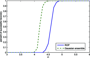
Figure 1: Rates of successful recovery for the ROP and Gaussian ensemble with $p_{1}=p_{2}=100$, $r=5$, and $n=Cr\max(p_{1},p_{2})$ for $C$ ranging from 3 to 6.

The numerical results show that for ROP from the Gaussian distribution, the minimum constant $C$ to ensure exact recovery with high probability is slightly less than 5 in the small scale problems ($p_{1},p_{2}\leq 100$) we tested. The corresponding minimum constant $C$ for the Gaussian ensemble is about $4.5$. Matrix completion requires much larger number of measurements. Based on the theoretical analyses given in CandesRecht , RechtImproved , the required number of measurements for matrix completion is $O(\mu r(p_{1}+p_{2})\log^{2}(p_{1}+p_{2}))$, where $\mu\geq 1$ is some coherence constant describing the “spikedness” of the matrix $A$. Hence, for matrix completion, the factor $C$ in (38) needs to grow with the dimensions $p_{1}$ and $p_{2}$ and it requires $C\gtrsim\mu\log^{2}(p_{1}+p_{2})$, which is much larger than what is needed for the ROP or Gaussian ensemble. The required storage space for the Gaussian ensemble is much greater than that for the ROP. In order to ensure accurate recovery of $p\times p$ matrices of rank $r$, one needs at least $4.5rp^{3}$ bytes of space to store the measurement matrices, which could be prohibitively large for the recovery of high-dimensional matrices. In contrast, the storage space for the projection vectors in ROP is only $10rp^{2}$ bytes, which is far smaller than what is required by the Gaussian ensemble in the high-dimensional case.

We then consider the recovery of approximately low-rank matrices to investigate the robustness of the method against small perturbations. To this end, we randomly draw $100\times 100$ matrix $A$ as $A=U\cdot\operatorname{diag}(1,2^{-1/2},\ldots,r^{-1/2})\cdot V^{\intercal}$, where $U\in\mathbb{R}^{100\times r}$ and $V\in\mathbb{R}^{100\times r}$ are random matrices with orthonormal columns. We then observe $n=2000$ random rank-one projections with the measurement vectors being i.i.d. Gaussian. Based on the observations, the nuclear minimization procedure (7) is applied to estimate $A$. The results for different values of $r$ are shown in Figure 2. It can be seen from the plot that in this setting one can exactly recover a matrix of rank at most 4 with 2000 measurements. However, when the rank $r$ of the true matrix $A$ exceeds 4, the estimate is still stable. The theoretical result in Proposition 2.1 bounds the loss (solid line) at $O(\|A_{-\max(4)}\|^{2}_{\ast}/4)$ (shown in the dashed line) with high probability, which corresponds to Figure 2.

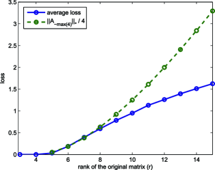
Figure 2: Recovery accuracy (solid line) for approximately low-rank matrices with different values of $r$, where $p_{1}=p_{2}=100$, $n=2000$, $\sigma(A)=(1,1/\sqrt{2},\ldots,1/\sqrt{r})$. The dashed line is the theoretical upper bound.

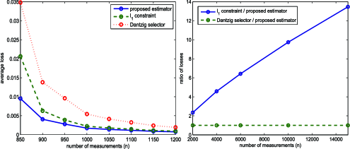
Figure 3: Left panel: Comparison of the proposed estimator with $\hat{A}{}^{\ell_{1}}$ and $\hat{A}{}^{\mathrm{DS}}$ for $p_{1}=p_{2}=50$, $r=4$, $\sigma=0.01$, and $n$ ranging from 850 to 1200. Right panel: Ratio of the squared Frobenius norm loss of $\hat{A}{}^{\ell_{1}}$ to that of the proposed estimator for $p_{1}=p_{2}=50$, $r=4$, and $n$ varying from 2000 to 15,000.

We now turn to the noisy case. The low-rank matrices $A$ are generated by $A=X^{\intercal}Y$, where $X\in\mathbb{R}^{r\times p_{1}}$ and $Y\in\mathbb{R}^{r\times p_{2}}$ are i.i.d. Gaussian matrices. The ROP $\mathcal{X}$ is from the standard Gaussian distribution and the noise vector $z\sim N_{n}(0,\sigma^{2})$. Based on $(\mathcal{X},y)$ with $y=\mathcal{X}(A)+z$, we compare our proposed estimator $\hat{A}$ with the $\ell_{1}$ constraint minimization estimator $\hat{A}{}^{\ell_{1}}$ Chen and the matrix Dantzig Selector $\hat{A}{}^{\mathrm{DS}}$ CandesOracle , where

$$\hat{A} = \mathop{\arg\min}_{M}\bigl{\{}\|M\|_{\ast}\dvtx y-\mathcal{X}(M)\in\mathcal{Z}_{1}\cap\mathcal{Z}_{2}\bigr{\}},$$

$$\hat{A}{}^{\ell_{1}} = \mathop{\arg\min}_{M}\bigl{\{}\|M\|_{\ast}\dvtx y-\mathcal{X}(M)\in\mathcal{Z}_{1}\bigr{\}},$$

$$\hat{A}{}^{\mathrm{DS}} = \mathop{\arg\min}_{M}\bigl{\{}\|M\|_{\ast}\dvtx y-\mathcal{X}(M)\in\mathcal{Z}_{2}\bigr{\}},$$

with $\mathcal{Z}_{1}=\{z\dvtx\|z\|_{1}/n\leq\sigma\}$ and $\mathcal{Z}_{2}=\{z\dvtx\|\mathcal{X}(z)\|\leq\sigma(\sqrt{\log n}(p_{1}+p_{2})+\break\sqrt{n(p_{1}+p_{2})})\}$. Note that $\hat{A}{}^{\ell_{1}}$ is similar to the estimator proposed in Chen et al. Chen , except their estimator is for symmetric matrices under the SROP but ours is for general low-rank matrices under the ROP. Figure 3 compares the performance of the three estimators. It can be seen from the left panel that for small $n$, $\ell_{1}$ constrained minimization outperforms the matrix Dantzig Selector, while our estimator outperforms both $\hat{A}{}^{\ell_{1}}$ and $\hat{A}{}^{\mathrm{DS}}$. When $n$ is large, our estimator and $\hat{A}{}^{\mathrm{DS}}$ are essentially the same and both outperforms $\hat{A}{}^{\ell_{1}}$. The right panel of Figure 3 plots the ratio of the squared Frobenius norm loss of $\hat{A}{}^{\ell_{1}}$ to that of our estimator. The ratio increases with $n$. These numerical results are consistent with the observations made in Remark 2.3.

We now turn to the recovery of symmetric low-rank matrices under the SROP model (18). Let $\mathcal{X}$ be SROP from the standard normal distribution. We consider the setting where $p=40$, $n$ varies from 50 to 600, $z_{i}\sim\sigma\cdot\mathcal{U}[-1,1]$ with $\sigma={}$0.1, 0.01, 0.001 or 0.0001, and $A$ is randomly generated as rank-5 matrix by the same procedure discussed above. The setting is identical to the one considered in Section 5.1 of Chen . Although we cannot exactly repeat the simulation study in Chen as they did not specify the choice of the tuning parameter, we can implement both our procedure

$$\hat{A} = \mathop{\arg\min}_{M}\biggl{\{}\|M\|_{\ast}\dvtx\bigl{\|}y-\mathcal{X}(M)\bigr{\|}_{1}\leq\frac{n\sigma}{2},$$

$$\hskip 39.0pt{}\bigl{\|}\tilde{\mathcal{X}}^{\ast}\bigl{(}\tilde{y}-\tilde{\mathcal{X}}(M)\bigr{)}\bigr{\|}\leq\frac{\sigma(\sqrt{\log n}p+\sqrt{np})}{3}\biggr{\}}$$

and the estimator $\hat{A}{}^{\ell_{1}}$ with only the $\ell_{1}$ constraint which was proposed by Chen et al. Chen

$$\hat{A}{}^{\ell_{1}}=\mathop{\arg\min}_{M}\biggl{\{}\|M\|_{\ast}\dvtx\bigl{\|}y-\mathcal{X}(M)\bigr{\|}_{1}\leq\frac{n\sigma}{2}\biggr{\}}.$$

The results are given in Figure 4. It can be seen that our estimator $\hat{A}$ outperforms the estimator $\hat{A}{}^{\ell_{1}}$.

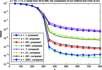
Figure 4: Comparison of the proposed estimator $\hat{A}$ with the $\hat{A}{}^{\ell_{1}}$. Here $p=40$, $r=5$, $\sigma=0.1,0.01,0.001,0.0001$ and $n$ ranges from 50 to 800.

5.1 Data driven selection of tuning parameters

We have so far considered the estimators

$$\hat{A} = \mathop{\arg\min}_{B}\bigl{\{}\|B\|_{\ast}\dvtx\bigl{\|}y-\mathcal{X}(B)\bigr{\|}_{1}/n\leq\lambda,\bigl{\|}\mathcal{X}^{\ast}\bigl{(}y-\mathcal{X}(B)\bigr{)}\bigr{\|}\leq\eta\bigr{\}},$$ (39)

$$\hat{A} = \mathop{\arg\min}_{M}\bigl{\{}\|M\|_{\ast}\dvtx\bigl{\|}y-\mathcal{X}(M)\bigr{\|}_{1}/n\leq\lambda,\bigl{\|}\tilde{\mathcal{X}}^{\ast}\bigl{(}\tilde{y}-\tilde{\mathcal{X}}(M)\bigr{)}\bigr{\|}\leq\eta\bigr{\}}$$ (40)

for the ROP and SROP, respectively. The theoretical choice of the tuning parameters $\lambda$ and $\eta$ depends on the knowledge of the error distribution such as the variance. In real applications, such information may not be available and/or the theoretical choice may not be the best. It is thus desirable to have a data driven choice of the tuning parameters. We now introduce a practical method for selecting the tuning parameters using $K$-fold cross-validation.

Let $(\mathcal{X},y)=\{(X_{i},y_{i}),i=1,\ldots,n\}$ be the observed sample and let $T$ be a grid of positive real values. For each $t\in T$, set

$$(\lambda,\eta) = \bigl{(}\lambda(t),\eta(t)\bigr{)}$$

$$= \cases{\bigl{(}t,t\bigl{(}\sqrt{\log n}(p_{1}+p_{2})+\sqrt{n(p_{1}+p_{2})}\bigr{)}\bigr{)},&\quad for ROP;\vspace*{5pt}\cr\bigl{(}t,t(\sqrt{\log n}p+\sqrt{np})\bigr{)},&\quad for SROP.}$$

Randomly split the $n$ samples $(X_{i},y_{i}),i=1,\ldots,n$ into two groups of sizes $n_{1}\sim\frac{(K-1)n}{K}$ and $n_{2}\sim\frac{n}{K}$ for $I$ times. Denote by $J_{1}^{i},J_{2}^{i}\subseteq\{1,\ldots,n\}$ the index sets for Groups 1 and 2, respectively, for the $i$th split. Apply our procedure [(39) for ROP and (40) for SROP, resp.] to the sub-samples in Group 1 with the tuning parameters $(\lambda(t),\eta(t))$ and denote the estimators by $\hat{A}{}^{i}(t)$, $i=1,\ldots,I$. Evaluate the prediction error of $\hat{A}{}^{i}(t)$ over the subsample in Group 2 and set

$$\hat{R}(t)=\sum_{i=1}^{I}\sum_{j\in J_{2}^{i}}\bigl{|}y_{j}-\bigl{\langle}A^{i}(t),X_{j}\bigr{\rangle}\bigr{|}^{2},\qquad t\in T.$$

We select

$$t_{*}=\mathop{\arg\min}_{T}\hat{R}(t)$$

and choose the tuning parameters $(\lambda(t_{*}),\eta(t_{*}))$ as in (5.1) with $t=t_{*}$ and the final estimator $\hat{A}$ based on (39) or (40) with the chosen tuning parameters.

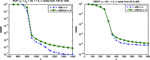
Figure 5: Comparison of the performance with cross validation and without cross-validation in both ROP and SROP. Left panel: ROP, $p_{1}=p_{2}=30$, $r=4$, $n$ varies from 750 to 1400. Right panel: SROP, $p=40$, $r=5$, $n$ varies from 50 to 800.

We compare the numerical result by 5-fold cross-validation with the result based on the known $\sigma$ by simulation in Figure 5. Both the ROP and SROP are considered. It can be seen that the estimator with the tuning parameters chosen through 5-fold cross-validation has the same performance as or outperforms the one with the theoretical choice of the tuning parameters.

5.2 Image compression

Since a two-dimensional image can be considered as a matrix, one approach to image compression is by using low-rank matrix approximation via the singular value decomposition. See, for example, Andrews , RechtMatrix , Wakinimage . Here, we use an image recovery example to further illustrate the nuclear norm minimization method under the ROP model.

For a grayscale image, let $A=(a_{i,j})\in\mathbb{R}^{m\times n}$ be the intensity matrix associated with the image, where $a_{ij}$ is the grayscale intensity of the $(i,j)$ pixel. When the matrix $A$ is approximately low-rank, the ROP model and nuclear norm minimization method can be used for image compression and recovery. To illustrate this point, let us consider the following grayscale MIT Logo image (Figure 6).

Figure 6: Original grayscale MIT logo.

The matrix associated with MIT logo is of the size $50\times 80$ and of rank 6. We take rank-one random projections $\mathcal{X}(A)$ as the observed sample, with various sample sizes. Then the constrained nuclear norm minimization method is applied to reconstruct the original low-rank matrix. The recovery results are shown in Figure 7. The results show that the original image can be compressed and recovered well via the ROP model and the nuclear norm minimization.

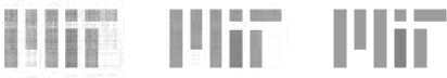
Figure 7: Recovery of MIT logo based on different number of measurements. Left: 900; Middle: 1000; Right: 1080.

6 Discussions

This paper introduces the ROP model for the recovery of general low-rank matrices. A constrained nuclear norm minimization method is proposed and its theoretical and numerical properties are studied. The proposed estimator is shown to be rate-optimal when the number of rank-one projections $n\gtrsim\log n(p_{1}+p_{2})$ or $n\sim r(p_{1}+p_{2})$. It is also shown that the procedure is adaptive to the rank and robust against small perturbations. The method and results are applied to estimation of a spiked covariance matrix. It is somewhat unexpected that it is possible to accurately recover a spiked covariance matrix from only one-dimensional projections. An interesting open problem is to estimate the principal components/subspace based on the one-dimensional random projections. We leave this as future work.

In a recent paper, Chen et al. Chen considered quadratic measurements for the recovery of symmetric positive definite matrices, which is similar to the special case of SROP that we studied here. The paper was posted on arXiv as we finish writing the present paper. They considered the noiseless and $\ell_{1}$ bounded noise cases and introduced the so-called “RIP-$\ell_{2}$/$\ell_{1}$” condition. The “RIP-$\ell_{2}$/$\ell_{1}$” condition is similar to RUB in our work. But these two conditions are not identical as the RIP-$\ell_{2}$/$\ell_{1}$ condition can only be applied to symmetric low-rank matrices as only symmetric operators are considered in the paper. In contrast, RUB applies to all low-rank matrices.

Chen et al. (Chen version 4) considered $\ell_{1}$-bounded noise case under the SROP model and gave an upper bound in their Theorem 3 (after a slight change of notation)

$$\|\hat{\Sigma}-\Sigma\|_{F}\leq C_{1}\frac{\|\Sigma-\Sigma_{\Omega}\|_{\ast}}{\sqrt{r}}+C_{2}\frac{\varepsilon}{n}.$$ (42)

This result for $\ell_{1}$ bounded noise case is not applicable to the i.i.d. random noise setting. When the entries of the noise term $\eta\in\mathbb{R}^{n}$ are of constant order, which is the typical case for i.i.d. noise with constant variance, one has $\|\eta\|_{1}\sim Cn$ with high probability. In such a case, the term $C_{2}\frac{\varepsilon_{1}}{n}$ on the right-hand side of (42) does not even converge to 0 as the sample size $n\to\infty$.

In comparison, the bound (30) in Proposition 3.1 can be equivalently rewritten as

$$\qquad\|\hat{A}-A\|_{F}\leq W_{2}\frac{\|A_{-\max(r)}\|_{\ast}}{\sqrt{r}}+W_{1}\tau\min\biggl{(}\frac{\sqrt{r\log n}p}{n}+\sqrt{\frac{rp}{n}},1\biggr{)},$$ (43)

where the first term $W_{2}\frac{\|A_{-\max(r)}\|_{\ast}}{\sqrt{r}}$ is of the same order as $C_{1}\frac{\|\Sigma-\Sigma_{\Omega}\|_{\ast}}{\sqrt{r}}$ in (42) while the second term decays to 0 as $n\to\infty$. Hence, for the recovery of rank-$r$ matrices, as the sample size $n$ increases our bound decays to 0 but the bound (42) given in Chen et al. Chen does not. The main reason of this phenomenon lies in the difference in the two methods: we use nuclear norm minimization under two convex constraints (see Remark 2.3), but Chen et al. Chen used only the $\ell_{1}$ constraint. Both theoretical results (see Remark 2.3) and numerical results (Figure 3 in Section 5) show that the additional constraint $\mathcal{Z}_{2}$ improves the performance of the estimator.

Moreover, the results and techniques in Chen for symmetric positive definite matrices are not applicable to the recovery of general nonsymmetric matrices. This is due to the fact that for a nonsymmetric square matrix $A=(a_{ij})$, the quadratic measurements $(\beta^{(i)})^{\intercal}A\beta^{(i)}$ satisfy

$$\bigl{(}\beta^{(i)}\bigr{)}^{\intercal}A\beta^{(i)}=\bigl{(}\beta^{(i)}\bigr{)}^{\intercal}A^{s}\beta^{(i)},$$

where $A^{s}={1\over 2}(A+A^{\intercal})$. Hence, for a nonsymmetric matrix $A$, only its symmetrized version $A^{s}$ can be possibly identified and estimated based on the quadratic measurements, the matrix $A$ itself is neither identifiable nor estimable.

7 Proofs

We prove the main results in this section. We begin by collecting a few important technical lemmas that will be used in the proofs of the main results. The proofs of some of these technical lemmas are involved and are postponed to the supplementary material Supplement .

7.1 Technical tools

Lemmas 7.1 and 7.2 below are used for deriving the RUB condition (see Definition 2.1) from the ROP design.

Lemma 7.1.

Suppose $A\in\mathbb{R}^{p_{1}\times p_{2}}$ is a fixed matrix and $\mathcal{X}$ is ROP from a symmetric sub-Gaussian distribution $\mathcal{P}$, that is,

$$\bigl{[}\mathcal{X}(A)\bigr{]}_{j}=\beta^{(j)T}A\gamma^{(j)},\qquad j=1,\ldots,n,$$

where $\beta^{(j)}=(\beta_{1}^{(j)},\ldots,\beta_{p_{1}}^{(j)})^{T},\gamma^{(j)}=(\gamma_{1}^{(j)},\ldots,\gamma_{p_{2}}^{(j)})^{T}$ are random vectors with entries i.i.d. generated from $\mathcal{P}$. Then for $\delta>0$, we have

$$\biggl{(}\frac{1}{3\alpha^{4}_{\mathcal{P}}}-2\alpha^{2}_{\mathcal{P}}\delta-\alpha^{2}_{\mathcal{P}}\delta^{2}\biggr{)}\|A\|_{F}\leq\bigl{\|}\mathcal{X}(A)\bigr{\|}_{1}/n\leq\bigl{(}1+2\alpha_{\mathcal{P}}^{2}\delta+\alpha_{\mathcal{P}}^{2}\delta^{2}\bigr{)}\|A\|_{F}$$

with probability at least $1-2\exp(-\delta^{2}n)$. Here, $\alpha_{\mathcal{P}}$ is defined by (26).

Lemma 7.2.

Suppose $A\in\mathbb{R}^{p_{1}\times p_{2}}$ is a fixed matrix. $\beta=(\beta_{1},\ldots,\beta_{p_{1}})^{T},\gamma=(\gamma_{1},\ldots,\gamma_{p_{2}})^{T}$ are random vectors such that $\beta_{1},\ldots,\beta_{p_{1}},\gamma_{1},\ldots,\gamma_{p_{2}}\stackrel{{\scriptstyle\mathit{i.i.d.}}}{{\sim}}\mathcal{P}$, where $\mathcal{P}$ is some symmetric variance 1 sub-Gaussian distribution, then we have

$$\frac{\|A\|_{F}}{3\alpha^{4}_{\mathcal{P}}}\leq E\bigl{|}\beta^{T}A\gamma\bigr{|}\leq\|A\|_{F},$$

where $\alpha_{\mathcal{P}}$ is given by (26).

Let $z\in\mathbb{R}^{n}$ be i.i.d. sub-Gaussian distributed. By measure concentration theory, $\|z\|_{p}^{p}/n$, $1\leq p\leq\infty$, are essentially bounded; specifically, we have the following lemma.

Lemma 7.3.

Suppose $z\in\mathbb{R}^{n}$ and $z_{i}\stackrel{{\scriptstyle\mathit{i.i.d.}}}{{\sim}}N(0,\sigma^{2})$, we have

$$P\bigl{(}\|z\|_{1}\geq\sigma n\bigr{)} \leq \frac{9}{n},$$

$$P\bigl{(}\|z\|_{2}\geq\sigma\sqrt{n+2\sqrt{n\log n}}\bigr{)} \leq \frac{1}{n},$$

$$P\bigl{(}\|z\|_{\infty}\geq 2\sigma\sqrt{\log n}\bigr{)} \leq \frac{1}{n\sqrt{2\pi\log n}}.$$

More general, when $z_{i}$ are i.i.d. sub-Gaussian distributed such that (25) holds, then

$$P\bigl{(}\|z\|_{1}\geq Cn\bigr{)} \leq \exp\biggl{(}-\frac{n(C-2\sqrt{2\pi}\gamma)^{2}}{2\gamma^{2}}\biggr{)}\qquad\forall C>2\sqrt{2\pi}\gamma,$$

$$P\bigl{(}\|z\|_{2}\geq\sqrt{Cn}\bigr{)} \leq \exp\biggl{(}-\frac{n(C-4\gamma^{2})^{2}}{8\gamma^{2}C}\biggr{)}\qquad\forall C>4\gamma^{2},$$

$$P\bigl{(}\|z\|_{\infty}\geq C\gamma\sqrt{\log n}\bigr{)} \leq 2n^{-C^{2}/2-1}\qquad\forall C>0.$$

Lemma 7.4 below presents an upper bound for the spectral norm of $\mathcal{X}(z)$ for a fixed vector $z$.

Lemma 7.4.

Suppose $\mathcal{X}$ is ROP from some symmetric sub-Gaussian distribution $\mathcal{P}$ and $z\in\mathbb{R}^{n}$ is some fixed vector, then for $C>\log 7$, we have

$$\bigl{\|}\mathcal{X}^{\ast}(z)\bigr{\|}\leq 3\alpha_{\mathcal{P}}^{2}\bigl{(}C(p_{1}+p_{2})\|z\|_{\infty}+\sqrt{2C(p_{1}+p_{2})}\|z\|_{2}\bigr{)}$$

with probability at least $1-2\exp(-(C-\log 7)(p_{1}+p_{2}))$. Here, $\alpha_{\mathcal{P}}$ is defined by (26).

We are now ready to prove the main results of the paper.

7.2 Proof of Theorem 2.1

We introduce the following two technical lemmas that will be used in the proof of theorem.

The null space property below is a well-known result in affine rank minimization problem (see Oymak11 ). It provides a necessary, sufficient and easier-to-check condition for exact recovery in the noiseless setting.

Lemma 7.5 ((Null space property)).

Using (7), one can recover all matrices $A$ of rank at most $r$ if and only if for all $R\in\mathcal{N}(\mathcal{X})\setminus\{0\}$,

$$\|R_{\max(r)}\|_{\ast}<\|R_{-\max(r)}\|_{\ast}.$$

The following lemma is given in CaiZhang3 , which provides a way to decompose the general vectors to sparse ones.

Lemma 7.6 ((Sparse representation of a polytope)).

Suppose $s$ is a nonnegative integer, $v\in\mathbb{R}^{p}$ and $\theta\geq 0$. Then $\|v\|_{\infty}\leq\theta,\|v\|_{1}\leq s\theta$, if and only if $v$ can be expressed as a weighted mean,

$$v=\sum_{i=1}^{N}\lambda_{i}u_{i},\qquad 0\leq\lambda_{i}\leq 1,\qquad\sum_{i=1}^{N}\lambda_{i}=1,$$

where $u_{i}$ satisfies

$$u_{i}\mbox{ is $s$-sparse},\qquad\operatorname{supp}(u_{i})\subseteq\operatorname{supp}(v),$$

(44)

$$\|u_{i}\|_{1}=\|v\|_{1},\qquad\|u_{i}\|_{\infty}\leq\theta.$$

For the proof of Theorem 2.1, by null space property (Lemma 7.5), we only need to show for all nonzero $R$ with $\mathcal{X}(R)=0$, we must have $\|R_{\max(r)}\|_{\ast}<\|R_{-\max(r)}\|_{\ast}$.

If this does not hold, suppose there exists nonzero $R$ with $\mathcal{X}(R)=0$ and $\|R_{\max(r)}\|_{\ast}\geq\|R_{-\max(r)}\|_{\ast}$. We denote $p=\min(p_{1},p_{2})$ and assume the singular value decomposition of $R$ is

$$R=\sum_{i=1}^{p}\sigma_{i}u_{i}v_{i}^{\intercal}=U\operatorname{diag}(\vec{\sigma})V^{\intercal},$$

where $u_{i}$, $v_{i}$ are orthogonal basis in $\mathbb{R}^{p_{1}}$, $\mathbb{R}^{p_{2}}$, respectively, and $\vec{\sigma}$ is the singular value vector such that $\sigma_{1}\geq\sigma_{2}\geq\cdots\geq\sigma_{p}\geq 0$. Without loss of generality, we can assume $p\geq kr$, otherwise we can set the undefined entries of $\sigma$ as $0$.

Consider the singular value vector $\vec{\sigma}=(\sigma_{1},\sigma_{2},\ldots,\sigma_{p})$, we note that$\vec{\sigma}_{-\max(kr)}$ satisfies

$$\|\vec{\sigma}_{-\max(kr)}\|_{\infty} \leq \sigma_{kr},$$

$$\|\vec{\sigma}_{-\max(kr)}\|_{1} = \|\vec{\sigma}_{-\max(r)}\|_{1}-(\sigma_{r+1}+\cdots+\sigma_{kr})$$

$$\leq \|\vec{\sigma}_{-\max(r)}\|_{1}-(k-1)r\sigma_{kr}$$

$$\leq \|\vec{\sigma}_{\max(r)}\|_{1}-(k-1)r\sigma_{kr}.$$

Denote $\theta=\max\{\sigma_{kr},(\|\vec{\sigma}_{\max(r)}\|_{1}-r(k-1)\sigma_{kr})/(kr)\}$, by the two inequalities above we have $\|\vec{\sigma}_{-\max(kr)}\|_{\infty}\leq\theta$ and $\|\vec{\sigma}_{-\max(kr)}\|_{1}\leq kr\theta$. Now apply Lemma 7.6, we can get $b^{(i)}\in\mathbb{R}^{p},\lambda_{i}\geq 0,i=1,\ldots,N$ such that $\sum_{i=1}^{N}\lambda_{i}=1$, $\vec{\sigma}_{-\max(kr)}=\sum_{i=1}^{N}\lambda_{i}b^{(i)}$ and

$$\operatorname{supp}\bigl{(}b^{(i)}\bigr{)} \subseteq \operatorname{supp}(\vec{\sigma}_{-\max(kr)}),\qquad\bigl{\|}b^{(i)}\bigr{\|}_{0}\leq kr,$$

$$\bigl{\|}b^{(i)}\bigr{\|}_{1} = \|\vec{\sigma}_{-\max(kr)}\|_{1},\qquad\bigl{\|}b^{(i)}\bigr{\|}_{\infty}\leq\theta,$$

which leads to

$$\bigl{\|}b^{(i)}\bigr{\|}_{2}\leq\sqrt{\bigl{\|}b^{(i)}\bigr{\|}_{1}\cdot\bigl{\|}b^{(i)}\bigr{\|}_{\infty}}\leq\sqrt{\bigl{(}\|\vec{\sigma}_{\max(r)}\|_{1}-r(k-1)\sigma_{kr}\bigr{)}\cdot\theta}.$$

If $\theta=\sigma_{kr}$, we have

$$\bigl{\|}b^{(i)}\bigr{\|}_{2} \leq \sqrt{\bigl{(}\|\vec{\sigma}_{\max(r)}\|_{1}-r(k-1)\sigma_{kr}\bigr{)}\sigma_{kr}}$$

$$\leq \sqrt{\biggl{(}\|\vec{\sigma}_{\max(r)}\|_{1}-r(k-1)\frac{\|\vec{\sigma}_{\max(r)}\|_{1}}{2r(k-1)}\biggr{)}\frac{\|\vec{\sigma}_{\max(r)}\|_{1}}{2r(k-1)}}$$

$$\leq \frac{\|\vec{\sigma}_{\max(r)}\|_{1}}{\sqrt{4r(k-1)}}\leq\frac{\|\vec{\sigma}_{\max(r)}\|_{2}}{\sqrt{4(k-1)}}.$$

If $\theta=(\|\vec{\sigma}_{\max(r)}\|_{1}-r(k-1)\sigma_{kr})/(kr)$, we have

$$\bigl{\|}b^{(i)}\bigr{\|}_{2}\leq\sqrt{\frac{1}{kr}}\bigl{(}\|\vec{\sigma}_{\max(r)}\|_{1}-r(k-1)\sigma_{kr}\bigr{)}\leq\sqrt{\frac{1}{kr}}\|\vec{\sigma}_{\max(r)}\|_{1}\leq\frac{\|\vec{\sigma}_{\max(r)}\|_{2}}{\sqrt{k}}.$$

Since $k\geq 2$, we always have $\|b^{(i)}\|_{2}\leq\|\vec{\sigma}_{\max(r)}\|_{2}/\sqrt{k}$. Finally, we define $B_{i}=U\operatorname{diag}(b^{(i)})V^{\intercal}$, then the rank of $B_{i}$ are all at most $kr$ and $\sum_{i=1}^{N}\lambda_{i}B_{i}=R_{-\max(kr)}$ and

$$\|B_{i}\|_{F}=\bigl{\|}b^{(i)}\bigr{\|}_{2}\leq\|\vec{\sigma}_{\max(r)}\|_{2}/\sqrt{k}=\|R_{\max(r)}\|_{F}/\sqrt{k}.$$

Hence,

$$0 = \bigl{\|}\mathcal{X}(R)\bigr{\|}_{1}\geq\bigl{\|}\mathcal{X}(R_{\max(kr)})\bigr{\|}_{1}-\bigl{\|}\mathcal{X}(R_{-\max(kr)})\bigr{\|}_{1}$$

$$\geq C_{1}\|R_{\max(kr)}\|_{F}-\sum_{i=1}^{N}\bigl{\|}\mathcal{X}(\lambda_{i}B_{i})\bigr{\|}_{1}$$

$$\geq C_{1}\|R_{\max(r)}\|_{F}-\sum_{i=1}^{N}\lambda_{i}C_{2}\|B_{i}\|_{F}$$

$$\geq C_{1}\|R_{\max(r)}\|_{F}-C_{2}\|R_{\max(r)}\|_{F}/\sqrt{k}>0.$$

Here, we used the RUB condition. The last inequality is due to $C_{2}/C_{1}<\sqrt{k}$ and $R\neq 0$ (so $R_{\max(r)}\neq 0$). This is a contradiction, which completes the proof of the theorem.

7.3 Proof of Theorem 2.2

Notice that for $\mathcal{P}$ as standard Gaussian distribution, the constant $\alpha_{\mathcal{P}}$ [defined as (26)] equals $1$. We will prove the following more general result than Theorem 2.2 instead. The proof is provided in the supplementary material Supplement .

Proposition 7.1.

Suppose $\mathcal{X}\dvtx\mathbb{R}^{p_{1}\times p_{2}}\to\mathbb{R}^{n}$ is ROP from some variance 1 symmetric sub-Gaussian distribution $\mathcal{P}$. For integer $k\geq 2$, positive $C_{1}<\frac{1}{3\alpha^{4}_{\mathcal{P}}}$ [$\alpha_{\mathcal{P}}$ is defined as (26)] and $C_{2}>1$, there exists constants $C$ and $\delta$, only depending on $\mathcal{P},C_{1},C_{2}$ but not on $p_{1},p_{2},r$, such that if $n\geq Cr(p_{1}+p_{2})$, then with probability at least $1-e^{-n\delta}$, $\mathcal{X}$ satisfies RUB of order $kr$ and constants $C_{1}$ and $C_{2}$.

7.4 Proof of Theorems 2.3 and 3.1, Proposition 2.1

In order to prove the result, we introduce the following technical lemma as an extension of null space property (Lemma 7.5) from exact low-rank into the approximate low-rank setting.

Lemma 7.7.

Suppose $A_{\ast},A\in\mathbb{R}^{p_{1}\times p_{2}}$, $R=A_{\ast}-A$. If $\|A_{\ast}\|_{\ast}\leq\|A\|_{\ast}$, we have

$$\|R_{-\max(r)}\|_{\ast}\leq\|R_{\max(r)}\|_{\ast}+2\|A_{-\max(r)}\|_{\ast}.$$ (46)

The following two lemmas described the separate effect of constraint $\mathcal{Z}_{1}=\{z\dvtx\|z\|_{1}/n\leq\lambda_{1}\}$ and $\mathcal{Z}_{2}=\{z\dvtx\|\mathcal{X}^{\ast}(z)\|\leq\lambda_{2}\}$ on the estimator.

Lemma 7.8.

Suppose $\mathcal{X}$ satisfies RUB condition of order $kr$ with constants $C_{1},C_{2}$ such that $C_{1}>C_{2}/\sqrt{k}$. Assume that $A_{\ast},A\in\mathbb{R}^{p_{1}\times p_{2}}$ satisfy $\|A_{\ast}\|_{\ast}\leq\|A\|_{\ast}$, $\|\mathcal{X}(A_{\ast}-A)\|_{1}/n\leq\lambda_{1}$. Then we have

$$\|A_{\ast}-A\|_{F}\leq\frac{2}{C_{1}-C_{2}/\sqrt{k}}\lambda_{1}+\biggl{(}\frac{3}{\sqrt{k}C_{1}/C_{2}-1}+\frac{1}{\sqrt{k-1}}\biggr{)}\frac{\|A_{-\max(r)}\|_{\ast}}{\sqrt{r}}.$$

Lemma 7.9.

Suppose $\mathcal{X}$ satisfies RUB condition of order $kr$ with constants $C_{1},C_{2}$ such that $C_{1}>C_{2}/\sqrt{k}$. Assume that $\hat{A}{}^{\mathrm{DS}}$ satisfies $\|\mathcal{X}^{\ast}\mathcal{X}(A_{\ast}-A)\|\leq\lambda_{2}$. Then we have

$$\|A_{\ast}-A\|_{F} \leq \frac{4}{(C_{1}-C_{2}/\sqrt{k})^{2}}\cdot\frac{\sqrt{r}\lambda_{2}}{n}$$

$${}+\biggl{(}\frac{5}{\sqrt{k}C_{1}/C_{2}-1}+\frac{1}{\sqrt{k-1}}+1\biggr{)}\frac{\|A_{-\max(r)}\|_{\ast}}{\sqrt{r}}.$$

The proof of Lemmas 7.7, 7.8 and 7.9 are listed in the supplementary material Supplement . Now we prove Theorem 2.3 and Proposition 2.1. We only need to prove Proposition 2.1 since Theorem 2.3 is a special case of Proposition 2.1. By Lemmas 7.3 and 7.4, we have

$$P_{z}\bigl{(}\|z\|_{1}\leq\sigma n\bigr{)}\leq\frac{9}{n},$$

$$P_{\mathcal{X},z}\bigl{(}\bigl{\|}\mathcal{X}^{\ast}(z)\bigr{\|}\geq\sigma\bigl{(}12(p_{1}+p_{2})\sqrt{\log n}+6\sqrt{2(p_{1}+p_{2})n}\bigr{)}\bigr{)}$$

$$\qquad\leq P_{\mathcal{X}}\bigl{(}\bigl{\|}\mathcal{X}^{\ast}(z)\bigr{\|}\geq\bigl{(}6(p_{1}+p_{2})\|z\|_{\infty}+6\sqrt{p_{1}+p_{2}}\|z\|_{2}\bigr{)}\bigr{)}$$

$$\quad\qquad{}+P_{z}\bigl{(}\|z\|_{\infty}\geq 2\sigma\sqrt{\log n}\bigr{)}+P_{z}\bigl{(}\|z\|_{2}\geq\sigma\sqrt{2n}\bigr{)}$$

$$\qquad\leq 2\exp\bigl{(}-(2-\log 7)(p_{1}+p_{2})\bigr{)}+\frac{1}{n\sqrt{2\pi\log n}}+\frac{1}{n}.$$

Here, $P_{\mathcal{X}}$ ($P_{z}$ or $P_{\mathcal{X},z}$) means the probability with respect to $\mathcal{X}$ [$z$ or $(\mathcal{X},z)$]. Hence, we have

$$P(z\in\mathcal{Z}_{1}\cap\mathcal{Z}_{2})\geq 1-2\exp\bigl{(}-(2-\log 7)(p_{1}+p_{2})\bigr{)}-\frac{11}{n}.$$

Under the event that $z\in\mathcal{Z}_{1}\cap\mathcal{Z}_{2}$, $A$ is in the feasible set of the programming (12), which implies $\|\hat{A}\|_{\ast}\leq\|A\|_{\ast}$ by the definition of $\hat{A}$. Moreover, we have

$$\bigl{\|}\mathcal{X}(\hat{A}-A)\bigr{\|}_{1}/n \leq \bigl{\|}y-\mathcal{X}(A)\bigr{\|}_{1}/n+\bigl{\|}y-\mathcal{X}(\hat{A})\bigr{\|}_{1}/n$$

$$\leq \|z\|_{1}/n+\bigl{\|}y-\mathcal{X}(\hat{A})\bigr{\|}_{1}/n\leq 2\sigma,$$

$$\bigl{\|}\mathcal{X}^{\ast}\mathcal{X}(\hat{A}-A)\bigr{\|} \leq \bigl{\|}\mathcal{X}^{\ast}\bigl{(}y-\mathcal{X}(\hat{A})\bigr{)}\bigr{\|}+\bigl{\|}\mathcal{X}^{\ast}\bigl{(}y-\mathcal{X}(A)\bigr{)}\bigr{\|}$$

$$\leq \bigl{\|}\mathcal{X}^{\ast}\bigl{(}y-\mathcal{X}(\hat{A})\bigr{)}\bigr{\|}+\bigl{\|}\mathcal{X}^{\ast}(z)\bigr{\|}\leq 2\eta.$$

On the other hand, suppose $k=10$, by Theorem 2.2, we can have find a uniform constant $C$ and $\delta$ such that if $n\geq Crk(p_{1}+p_{2})$, $\mathcal{X}$ satisfies RUB of order $10r$ and constants $C_{1}=0.32,C_{2}=1.02$ with probability at least $1-e^{-n\delta^{\prime}}$. Hence, we have $D(=Ck)$ and $\delta^{\prime}$ such that if $n\geq Dr(p_{1}+p_{2})$, $\mathcal{X}$ satisfies RUB of order $10r$ and constants $C_{1},C_{2}$ satisfying $C_{2}/C_{1}<\sqrt{10}$ with probability at least $1-e^{-n\delta^{\prime}}$.

Now under the event that: [2.]

$\mathcal{X}$ satisfies RUB of order $10r$ and constants $C_{1},C_{2}$ satisfying $C_{2}/C_{1}<\sqrt{10}$,

$z\in\mathcal{Z}_{1}\cap\mathcal{Z}_{2}$, apply Lemmas 7.8 and 7.9 with $A_{\ast}=\hat{A}$, we can get (2.1). The probability that these two events both happen is at least $1-2\exp(-(2-\log 7)(p_{1}+p_{2}))-\frac{11}{n}-\exp(-\delta^{\prime}n)$. Set $\delta=\min(2-\log 7,\delta^{\prime})$, we finished the proof of Proposition 2.1.

For Theorem 3.1, the proof is similar. We apply the latter part of Lemmas 7.3 and 7.4 and get

$$P(z\notin\mathcal{Z}_{1}\cap\mathcal{Z}_{2})$$

$$\qquad\leq P\bigl{(}\|z\|_{1}/n>6\tau\bigr{)}$$

$$\quad\qquad{}+P\bigl{(}\bigl{\|}\mathcal{X}(z)\bigr{\|}>\tau\alpha^{2}_{\mathcal{P}}\bigl{(}6\sqrt{6n(p_{1}+p_{2})}+12\sqrt{\log n}(p_{1}+p_{2})\bigr{)}\bigr{)}$$

$$\qquad\leq P\bigl{(}\|z\|/n>6\tau\bigr{)}+P\bigl{(}\|z\|_{2}>\sqrt{6n}\tau\bigr{)}+P\bigl{(}\|z\|_{\infty}>2\sqrt{\log n}\tau\bigr{)}$$

$$\quad\qquad{}+P_{\mathcal{X}}\bigl{(}\bigl{\|}\mathcal{X}(z)\bigr{\|}>\alpha_{\mathcal{P}}^{2}\bigl{(}6(p_{1}+p_{2})\|z\|_{\infty}+6\sqrt{p_{1}+p_{2}}\|z\|_{2}\bigr{)}\bigr{)}$$

$$\qquad\leq\exp\bigl{(}-n(6-2\sqrt{2\pi})^{2}/2\bigr{)}+\exp(-n/12)$$

$$\quad\qquad{}+\frac{2}{n}+2\exp\bigl{(}-(2-\log 7)(p_{1}+p_{2})\bigr{)}.$$

Besides, we choose $k>(3\alpha^{4}_{\mathcal{P}})^{2}$, then we can find $C_{1}<1/(3\alpha_{\mathcal{P}}^{4})$ and $C_{2}>1$ such that $C_{2}/C_{1}<\sqrt{k}$. Apply Proposition 7.1, there exists $C,\delta^{\prime}$ only depending on $\mathcal{P}$, $C_{1},C_{2}$ such that if $n\geq Ckr(p_{1}+p_{2})$, $\mathcal{X}$ satisfies RUB of order $kr$ with constants $C_{1}$ and $C_{2}$ with probability at least $1-\exp(-\delta^{\prime}(p_{1}+p_{2}))$. Note that $C_{1},C_{2}$ only depends on $\mathcal{P}$, we can conclude that there exist constants $D(=Ck),\delta^{\prime}$ only depending on $\mathcal{P}$ such that if $n\geq Dr(p_{1}+p_{2})$, $\mathcal{X}$ satisfies RUB of order $kr$ with constants $C_{1},C_{2}$ satisfying $C_{2}/C_{1}\leq\sqrt{k}$.

Similarly, to the proof of Proposition 2.1, under the event that: [2.]

$\mathcal{X}$ satisfies RUB of order $kr$ and constants $C_{1},C_{2}$ satisfying $C_{2}/C_{1}<\sqrt{k}$,

$z\in\mathcal{Z}_{1}\cap\mathcal{Z}_{2}$, we can get (3.1) (we shall note that $W_{1}$ depends on $\mathcal{P}$, so its value can also depend on $\alpha_{\mathcal{P}}$). The probability that those events happen is at least $1-2/n-5\exp(-\delta(p_{1}+p_{2}))$ for $\delta\leq\min((6-2\sqrt{2\pi})^{2}/2,1/12,2-\log 7,\delta^{\prime})$.

7.5 Proof of Theorem 2.4

Without loss of generality, we assume that $p_{1}\leq p_{2}$. We consider the class of rank-$r$ matrices

$$\mathcal{F}_{c}=\bigl{\{}A\in\mathbb{R}^{p_{1}\times p_{2}}\dvtx A_{ij}=0,\mbox{ whenever }i\geq r+1\bigr{\}}$$

namely the matrices with all nonzero entries in the first $r$ rows. The model (1) become

$$y_{i}=\beta_{1\dvtx r}^{(i)T}A_{r}\gamma^{(i)}+z_{i},\qquad i=1,\ldots,n,$$

where $\beta^{(i)}_{1\dvtx r}$ is the vector of the first to the $r$th entries of $\beta^{(i)}$. Note that this is a linear regression model with variable $A_{r}\in\mathbb{R}^{r\times p_{2}}$, by Lemma 3.11 in CandesOracle , we have

$$\inf_{\hat{A}}\sup_{A\in\mathcal{F}_{c}}E\bigl{\|}\hat{A}(y)-A\bigr{\|}_{F}^{2} = \sigma^{2}\operatorname{trace}\bigl{[}\bigl{(}\mathcal{X}_{r}^{\ast}\mathcal{X}_{r}\bigr{)}^{-1}\bigr{]},$$ (47)

$$\inf_{\hat{A}}\sup_{A\in\mathcal{F}_{c}}E\bigl{\|}\hat{A}(y)-A\bigr{\|}_{F}^{2} = \infty\qquad\mbox{when $\mathcal{X}_{r}^{\ast}\mathcal{X}_{r}$ is singular,}$$ (48)

where $\mathcal{X}_{r}\dvtx\mathbb{R}^{r\times p_{2}}\to\mathbb{R}^{n}$ is the $\mathcal{X}$ constrained on $\mathcal{F}_{c}$, Then $\mathcal{X}_{r}$ sends $A_{r}$ to $(\beta^{(1)}_{1\dvtx r}A_{r}\gamma^{(1)},\ldots,\beta^{(n)}_{1\dvtx r}A_{r}\gamma^{(n)})^{\intercal}$. When $n<p_{2}r$, $\mathcal{X}_{r}$ is singular, hence we have (16).

When $n\geq p_{2}r$, we can see in order to show (15), we only need to show $\operatorname{trace}(\mathcal{X}_{r}^{\ast}\mathcal{X}_{r})\geq\frac{p_{2}r}{2n}$ with probability at least $1-26n^{-1}$. Suppose the singular value of $\mathcal{X}_{r}$ are $\sigma_{i}(\mathcal{X}_{r})$, $i=1,\ldots,rp_{2}$, then $\operatorname{trace}(\mathcal{X}_{r}^{\ast}\mathcal{X}_{r})=\sum_{i=1}^{p_{2}r}\sigma^{-2}(\mathcal{X}_{r})$.

Suppose $\mathcal{X}$ is ROP while $B\in\mathbb{R}^{r\times p_{2}}$ is i.i.d. standard Gaussian random matrix (both $\mathcal{X}$ and $B_{r}$ are random). Then by some calculation, we can see

$$E_{B,\mathcal{X}_{r}}\bigl{\|}\mathcal{X}_{r}(B)\bigr{\|}_{2}^{2}=nE_{B,\beta,\gamma}\bigl{(}\beta_{1\dvtx r}^{\intercal}B\gamma\bigr{)}^{2}=n\sum_{j=1}^{r}\sum_{k=1}^{p_{2}}E(\beta_{j}B_{jk}\gamma_{k})^{2}=np_{2}r.$$

Note (0.20) in the proof of Lemma 7.1 in the supplementary material Supplement , we know $E(\beta_{1\dvtx r}^{(i)T}B\gamma^{(i)}\|_{2}^{4}|B)\leq 9\|B\|_{F}^{4}$. Hence,

$$E\bigl{\|}\mathcal{X}_{r}(B)\bigr{\|}_{2}^{4} = \sum_{i=1}^{n}E\bigl{(}\beta_{1\dvtx r}^{(i)T}B\gamma^{(i)}\bigr{)}^{4}$$

$${}+2\sum_{1\leq i<l\leq n}E\sum_{j=1}^{n}\bigl{(}\beta_{1\dvtx r}^{(i)T}B\gamma^{(i)}\bigr{)}^{2}\cdot E\sum_{j=1}^{n}\bigl{(}\beta_{1\dvtx r}^{(l)T}B\gamma^{(l)}\bigr{)}^{2}$$

$$= n\cdot 9E\|B\|_{F}^{4}+n(n-1)(p_{2}r)^{2}$$

$$= 9nE\bigl{(}\chi^{2}(p_{2}r)\bigr{)}^{2}+n(n-1)p_{2}^{2}r^{2}$$

$$= 9n\bigl{(}p_{2}^{2}r^{2}+2p_{2}r\bigr{)}+n(n-1)p_{2}^{2}r^{2}$$

$$= n^{2}p_{2}^{2}r^{2}+2np_{2}r(4p_{2}r+9)\leq n^{2}p_{2}^{2}r^{2}+26np_{2}^{2}r_{2}^{2}.$$

Besides,

$$E\bigl{\|}\mathcal{X}_{r}(B_{r})\bigr{\|}_{2}^{2} = E\bigl{(}E\bigl{(}\bigl{\|}\mathcal{X}_{r}(B_{r})\bigr{\|}_{2}^{2}|\mathcal{X}_{r}\bigr{)}\bigr{)}=E\Biggl{(}\sum_{i=1}^{rp_{2}}\sigma_{i}^{2}(\mathcal{X}_{r})\Biggr{)},$$

$$E\bigl{\|}\mathcal{X}_{r}(B_{r})\bigr{\|}_{2}^{4} = E\bigl{(}E\bigl{(}\bigl{\|}\mathcal{X}_{r}(B_{r})\bigr{\|}_{2}^{4}|\mathcal{X}_{r}\bigr{)}\bigr{)}$$

$$= E\Biggl{(}\sum_{i=1}^{rp_{2}}3\sigma_{i}^{4}(\mathcal{X}_{r})+2\sum_{1\leq i<j\leq rp_{2}}\sigma_{i}^{2}(\mathcal{X}_{r})\sigma_{j}^{2}(\mathcal{X}_{r})\Biggr{)}$$

$$\geq E\Biggl{(}\sum_{i=1}^{rp_{2}}\sigma_{i}^{2}(\mathcal{X}_{r})^{2}\Biggr{)}^{2}.$$

Hence,

$$E\Biggl{(}\sum_{i=1}^{rp_{2}}\sigma_{i}^{2}(\mathcal{X}_{r})^{2}\Biggr{)} = np_{2}r,$$

$$\operatorname{Var}\Biggl{(}\sum_{i=1}^{rp_{2}}\sigma_{i}^{2}(\mathcal{X}_{r})^{2}\Biggr{)} = E\Biggl{(}\sum_{i=1}^{rp_{2}}\sigma_{i}^{2}(\mathcal{X}_{r})^{2}\Biggr{)}^{2}-\Biggl{(}E\sum_{i=1}^{rp_{2}}\sigma_{i}^{2}(\mathcal{X}_{r})^{2}\Biggr{)}^{2}\leq 26np_{2}^{2}r^{2}.$$

Then by Chebyshev’s inequality, we have

$$\sum_{i=1}^{rp_{2}}\sigma_{i}^{2}(\mathcal{X}_{r})\leq 2np_{2}r$$ (49)

with probability at least $1-\frac{26np_{2}^{2}r^{2}}{(npr)^{2}}=1-\frac{26}{n}$. By Cauchy–Schwarz’s inequality, we have

$$\operatorname{trace}\bigl{(}\bigl{(}\mathcal{X}_{r}^{\ast}\mathcal{X}_{r}\bigr{)}^{-1}\bigr{)}=\sum_{i=1}^{rp_{2}}\sigma_{i}^{-2}(\mathcal{X}_{r})\geq\frac{(p_{2}r)^{2}}{\sum_{i=1}^{rp_{2}}\sigma_{i}^{2}(\mathcal{X}_{r})}.$$

Therefore, we have

$$\operatorname{trace}\bigl{(}\bigl{(}\mathcal{X}_{r}^{\ast}\mathcal{X}_{r}\bigr{)}^{-1}\bigr{)}\geq\frac{p_{2}r}{2n}$$

with probability at least $1-26/n$, which shows (15).

Finally, we consider (14). Suppose inequality (49) holds, then

$$\bigl{|}\bigl{\{}i\dvtx\sigma_{i}^{2}(X_{r})\geq 4n\bigr{\}}\bigr{|}\leq\frac{p_{2}r}{2}$$

$$\qquad\Rightarrow\quad\biggl{|}\biggl{\{}i\dvtx\sigma_{i}^{-2}(X_{r})\leq\frac{1}{4n}\biggr{\}}\biggr{|}\geq\frac{p_{2}r}{2}$$ (50)

$$\qquad\Rightarrow\quad\biggl{|}\biggl{\{}i\dvtx\sigma_{i}^{-2}(X_{r})\geq\frac{1}{4n}\biggr{\}}\biggr{|}\geq\frac{p_{2}r}{2}.$$

By Lemma 3.12 in CandesOracle , we know

$$\inf_{\hat{A}}\sup_{A\in\mathcal{F}_{c}}P_{z}\biggl{(}\|\hat{A}-A\|_{F}^{2}\geq\frac{p_{2}r\sigma^{2}}{16n}\biggr{)}$$

$$\qquad=\inf_{\hat{A}}\sup_{A\in\mathcal{F}_{c}}E_{z}1_{\{x\geq p_{2}r\sigma^{2}/16n\}}\bigl{(}\|\hat{A}-A\|_{F}^{2}\bigr{)}$$

$$\qquad=E_{z}1_{\{x\geq p_{2}r\sigma^{2}/16n\}}\bigl{(}\bigl{\|}\bigl{(}\mathcal{X}_{r}^{\ast}\mathcal{X}_{r}\bigr{)}^{-1}\mathcal{X}_{r}^{\ast}(z)\bigr{\|}_{F}^{2}\bigr{)}$$

$$\qquad=P_{z}\biggl{(}\bigl{\|}\bigl{(}\mathcal{X}_{r}^{\ast}\mathcal{X}_{r}\bigr{)}^{-1}\mathcal{X}_{r}^{\ast}(z)\bigr{\|}_{F}^{2}\geq\frac{p_{2}r\sigma^{2}}{16n}\biggr{)},$$

where $1_{\{x\geq p_{2}r\sigma^{2}/16n\}}(\cdot)$ is the indicator function. Note that when $z\stackrel{{\scriptstyle\mathrm{i.i.d.}}}{{\sim}}\break N(0,\sigma^{2})$, $\|(\mathcal{X}_{r}^{\ast}\mathcal{X}_{r})^{-1}\mathcal{X}_{r}^{\ast}(z)\|_{F}^{2}$ is identical distributed as $\sum_{i=1}^{rp_{2}}\frac{y_{i}^{2}}{\sigma_{i}^{2}(\mathcal{X}_{r})}$, where $y_{1},\ldots,\break y_{rp_{2}}\stackrel{{\scriptstyle\mathrm{i.i.d.}}}{{\sim}}N(0,\sigma^{2})$, hence,

$$P\biggl{(}\bigl{\|}\bigl{(}\mathcal{X}_{r}^{\ast}\mathcal{X}_{r}\bigr{)}^{-1}\mathcal{X}_{r}^{\ast}(z)\bigr{\|}_{F}^{2}\leq\frac{p_{2}r\sigma^{2}}{16n}\biggr{)}$$

$$\qquad=P\Biggl{(}\sum_{i=1}^{rp_{2}}\frac{y_{i}^{2}}{\sigma_{i}^{2}(\mathcal{X}_{r})}\leq\frac{p_{2}r\sigma^{2}}{16n}\Biggr{)}$$

$$\qquad\leq P\biggl{(}\sum_{i\dvtx\sigma_{i}^{-2}(\mathcal{X}_{r})\geq 1/(4n)}y_{i}^{2}\sigma_{i}^{-2}(\mathcal{X}_{r})\leq\frac{p_{2}r\sigma^{2}}{16n}\biggr{)}$$

$$\qquad\leq P\biggl{(}\sum_{i\dvtx\sigma_{i}^{-2}(\mathcal{X}_{r})\geq 1/(4n)}\frac{y_{i}^{2}}{4n}\leq\frac{p_{2}r\sigma^{2}}{16n}\biggr{)}\leq P\biggl{(}\chi^{2}\biggl{(}\biggl{\lceil}\frac{rp_{2}}{2}\biggr{\rceil}\biggr{)}\leq\frac{p_{2}r}{4}\biggr{)}$$

$$\qquad\leq\exp\biggl{(}-\frac{rp_{2}}{32}\biggr{)}.$$

The last inequality is due to the tail bound of $\chi^{2}$ distribution given by Lemma 1 in Laurent ; the second last inequality is due to (7.5). In summary, when (49) holds, we have

$$\inf_{\hat{A}}\sup_{A\in\mathcal{F}_{c}}P_{z}\biggl{(}\|\hat{A}-A\|_{F}^{2}\geq\frac{p_{2}r\sigma^{2}}{16n}\biggr{)}\leq\exp\biggl{(}-\frac{rp_{2}}{32}\biggr{)}.$$

Finally, since $p_{2}\geq(p_{1}+p_{2})/2$, we showed that with probability at least $1-26n^{-1}$, $\mathcal{X}$ satisfies (14).

7.6 Proof of Theorem 4.1

We first introduce the following lemma about the upper bound of $\|z\|_{1},\|z\|_{2},\|z\|_{\infty}$.

Lemma 7.10.

Suppose $z$ is defined as (33), then for constants $C_{1}>\sqrt{2}$, $M_{1}>1$, we have

$$P\Biggl{(}\|z\|_{1}/n\leq\frac{C_{1}}{n}\sum_{i=1}^{n}\xi_{i}^{2}\Biggr{)} \geq 1-\frac{9C_{1}^{2}+6}{n(C_{1}-\sqrt{2})^{2}},$$

$$P\Biggl{(}\frac{C_{1}}{n}\sum_{i=1}^{n}\xi_{i}^{2}\leq M_{1}C_{1}\|\Sigma\|_{\ast}\Biggr{)} \geq 1-\frac{9}{n(M_{1}-1)^{2}};$$

for constants $C_{2}>1$, $M_{2}>9$,

$$P\biggl{(}\|z\|_{2}^{2}/n\leq\frac{C_{2}^{2}\sum_{i=1}^{n}\xi_{i}^{4}}{n}\biggr{)} \geq 1-\frac{105(105C_{2}^{4}+60)}{n(3C_{2}^{2}-2)^{2}},$$

$$P\biggl{(}\frac{C_{2}^{2}\sum_{i=1}^{n}\xi_{i}^{4}}{n}\leq M_{2}C_{2}^{2}\|\Sigma\|_{\ast}^{2}\biggr{)} \geq 1-\frac{105^{2}}{n(M_{1}-9)^{2}};$$

for constants $C_{3}>1$, $M_{3}>1$,

$$P\Bigl{(}\|z\|_{\infty}\leq C_{3}\log n\max_{1\leq i\leq n}\xi_{i}^{2}\Bigr{)}\geq 1-\frac{2}{\sqrt{2\pi C_{3}\log n}},$$

$$P\Bigl{(}C_{3}\log n\max_{1\leq i\leq n}\xi_{i}^{2}\leq 2C_{3}M_{3}\log^{2}n\bigl{(}\sqrt{\|\Sigma\|_{\ast}}+\sqrt{2M_{3}\log n\|\Sigma\|}\bigr{)}^{2}\Bigr{)}$$

$$\qquad\geq 1-2n^{-M_{3}+1}.$$

The proof of Lemma 7.10 is listed in the supplementary material Supplement . The rest of the proof is basically the same as Proposition 2.3. Suppose $\mathcal{X}_{1},\mathcal{X}_{2}$ and $\tilde{z}$ are given by (0.36), (0.37) and (0.39) in the supplementary material Supplement , then $\mathcal{X}_{1}$, $\mathcal{X}_{2}$ are ROP. By Lemma 7.4,

$$\bigl{\|}\mathcal{X}_{1}^{\ast}(\tilde{z})\bigr{\|} \leq 6\bigl{(}2p\|\tilde{z}\|_{\infty}+\sqrt{2p}\|\tilde{z}\|_{2}\bigr{)},$$ (54)

$$\bigl{\|}\mathcal{X}_{2}^{\ast}(\tilde{z})\bigr{\|} \leq 6\bigl{(}2p\|\tilde{z}\|_{\infty}+\sqrt{2p}\|\tilde{z}\|_{2}\bigr{)}$$ (55)

with probability at least $1-4\exp(-2(2-\log 7)p)$. Hence, there exists $\delta>0$ such that

$$P\bigl{(}\Sigma_{0}\mbox{ is NOT in the feasible set of (\ref{eqminimizationcovariance})}\bigr{)}$$

$$\qquad=P\bigl{(}\|z\|_{1}/n>\eta_{1}\mbox{ or }\bigl{\|}\tilde{\mathcal{X}}^{\ast}(\tilde{z})\bigr{\|}>\eta_{2}\bigr{)}$$

$$\qquad\leq P\Biggl{(}\|z\|_{1}/n>\frac{c_{1}}{n}\sum_{i=1}^{n}\xi_{i}^{2}\Biggr{)}+P\Bigl{(}\|\tilde{z}\|_{\infty}>2c_{3}\log n\max_{1\leq i\leq n}\xi_{i}^{2}\Bigr{)}$$

$$\quad\qquad{}+P\Biggl{(}\|\tilde{z}\|_{2}>c_{2}\sqrt{2\sum_{i=1}^{n}\xi_{i}^{4}}\Biggr{)}$$

$$\quad\qquad{}+P\bigl{(}\bigl{\|}\tilde{\mathcal{X}}^{\ast}(z)\bigr{\|}>24p\|\tilde{z}\|_{\infty}+12\sqrt{2p}\|\tilde{z}\|_{2}\bigr{)}$$

$$\qquad\leq P\Biggl{(}\|z\|_{1}/n>\frac{c_{1}}{n}\sum_{i=1}^{n}\xi_{i}^{2}\Biggr{)}+P\Bigl{(}\|z\|_{\infty}>c_{3}\log n\max_{1\leq i\leq n}\xi_{i}^{2}\Bigr{)}$$

$$\quad\qquad{}+P\Biggl{(}\|z\|_{2}>c_{2}\sqrt{\sum_{i=1}^{n}\xi_{i}^{4}}\Biggr{)}$$

$$\quad\qquad{}+P\bigl{(}\bigl{\|}\mathcal{X}^{\ast}_{1}(\tilde{z})\bigr{\|}>12p\|\tilde{z}\|_{\infty}+6\sqrt{2p}\|\tilde{z}\|_{2}\bigr{)}$$

$$\quad\qquad{}+P\bigl{(}\bigl{\|}\mathcal{X}^{\ast}_{2}(z)\bigr{\|}>12p\|\tilde{z}\|_{\infty}+6\sqrt{2p}\|\tilde{z}\|_{2}\bigr{)}$$

$$\qquad\leq O(1/n)+4\exp\bigl{(}-2(2-\log 7)p\bigr{)}+\frac{2}{\sqrt{2\pi c_{3}\log n}}.$$

Here, we used the fact that $\tilde{\mathcal{X}}^{\ast}=\mathcal{X}_{1}^{\ast}+\mathcal{X}_{2}^{\ast}$,

$$\|\tilde{z}\|_{2} = \sqrt{\sum_{i=1}^{\lfloor n/2\rfloor}(z_{2i-1}-z_{2i})^{2}}\leq\sqrt{\sum_{i=1}^{\lfloor n/2\rfloor}2\bigl{(}z_{2i-1}^{2}+z_{2i}^{2}\bigr{)}}\leq\sqrt{2}\|z\|_{2},$$

$$\|\tilde{z}\|_{\infty} = \max_{i}|z_{2i-1}-z_{2i}|\leq 2\max_{i}|z_{i}|\leq 2\|z\|_{\infty}.$$

Similarly to the proof of Proposition 2.3, since $\mathcal{X}_{1}$ is ROP, there exists constants $D$ and $\delta^{\prime}$ such that if $n\geq Drp$, $\mathcal{X}_{1}$ satisfies RUB of order $10k$ with constants $C_{1},C_{2}$ satisfying $C_{2}/C_{1}<\sqrt{10}$ with probability at least $1-e^{-n\delta^{\prime}}$.

Now under the event that: [3.]

$A$ is feasible in (34),

$\mathcal{X}_{1}$ satisfies RUB of order $10k$ with constants $C_{1},C_{2}$ satisfying $C_{2}/C_{1}<\sqrt{10}$,

the latter part of (7.10), (7.10) and (7.10) hold for some $M_{1}>1$, $M_{2}>9$, $M_{3}>2$, we can prove (4.1) similarly as the proof of Proposition 2.3, which we omit the proof here.

References

• (1) {barticle}[auto:parserefs-M02] \bauthor\bsnmAlquier, \bfnmP.\binitsP., \bauthor\bsnmButucea, \bfnmC.\binitsC., \bauthor\bsnmHebiri, \bfnmM.\binitsM. and \bauthor\bsnmMeziani, \bfnmK.\binitsK. (\byear2013). \btitleRank penalized estimation of a quantum system. \bjournalPhys. Rev. A. \bvolume88 \bpages032133. \bptokimsref\endbibitem
• (2) {barticle}[auto:parserefs-M02] \bauthor\bsnmAndrews, \bfnmH. C.\binitsH. C. and \bauthor\bsnmPatterson, \bfnmC. L.\binitsC. L. \bsuffixIII (\byear1976). \btitleSingular value decomposition (SVD) image coding. \bjournalIEEE Trans. Commun. \bvolume24 \bpages425–432. \bptokimsref\endbibitem
• (3) {barticle}[auto:parserefs-M02] \bauthor\bsnmBasri, \bfnmR.\binitsR. and \bauthor\bsnmJacobs, \bfnmD. W.\binitsD. W. (\byear2003). \btitleLambertian reflectance and linear sub-spaces. \bjournalIEEE Trans. Pattern Anal. Mach. Intell. \bvolume25 \bpages218–233. \bptokimsref\endbibitem
• (4) {barticle}[mr] \bauthor\bsnmBirnbaum, \bfnmAharon\binitsA., \bauthor\bsnmJohnstone, \bfnmIain M.\binitsI. M., \bauthor\bsnmNadler, \bfnmBoaz\binitsB. and \bauthor\bsnmPaul, \bfnmDebashis\binitsD. (\byear2013). \btitleMinimax bounds for sparse PCA with noisy high-dimensional data. \bjournalAnn. Statist. \bvolume41 \bpages1055–1084. \biddoi=10.1214/12-AOS1014, issn=0090-5364, mr=3113803 \bptokimsref\endbibitem
• (5) {barticle}[mr] \bauthor\bsnmCai, \bfnmT. Tony\binitsT. T., \bauthor\bsnmMa, \bfnmZongming\binitsZ. and \bauthor\bsnmWu, \bfnmYihong\binitsY. (\byear2013). \btitleSparse PCA: Optimal rates and adaptive estimation. \bjournalAnn. Statist. \bvolume41 \bpages3074–3110. \biddoi=10.1214/13-AOS1178, issn=0090-5364, mr=3161458 \bptokimsref\endbibitem
• (6) {barticle}[auto] \bauthor\bsnmCai, \bfnmT. Tony\binitsT. T., \bauthor\bsnmMa, \bfnmZongming\binitsZ. and \bauthor\bsnmWu, \bfnmYihong\binitsY. (\byear2014). \btitleOptimal estimation and rank detection for sparse spiked covariance matrices. \bjournalProbab. Theory Related Fields. \bnoteTo appear. \bptokimsref\endbibitem
• (7) {barticle}[mr] \bauthor\bsnmCai, \bfnmT. Tony\binitsT. T., \bauthor\bsnmXu, \bfnmGuangwu\binitsG. and \bauthor\bsnmZhang, \bfnmJun\binitsJ. (\byear2009). \btitleOn recovery of sparse signals via $\ell_{1}$ minimization. \bjournalIEEE Trans. Inform. Theory \bvolume55 \bpages3388–3397. \biddoi=10.1109/TIT.2009.2021377, issn=0018-9448, mr=2598028 \bptokimsref\endbibitem
• (8) {barticle}[mr] \bauthor\bsnmCai, \bfnmT. Tony\binitsT. T. and \bauthor\bsnmZhang, \bfnmAnru\binitsA. (\byear2013). \btitleSharp RIP bound for sparse signal and low-rank matrix recovery. \bjournalAppl. Comput. Harmon. Anal. \bvolume35 \bpages74–93. \biddoi=10.1016/j.acha.2012.07.010, issn=1063-5203, mr=3053747 \bptokimsref\endbibitem
• (9) {barticle}[mr] \bauthor\bsnmCai, \bfnmT. Tony\binitsT. T. and \bauthor\bsnmZhang, \bfnmAnru\binitsA. (\byear2013). \btitleCompressed sensing and affine rank minimization under restricted isometry. \bjournalIEEE Trans. Signal Process. \bvolume61 \bpages3279–3290. \biddoi=10.1109/TSP.2013.2259164, issn=1053-587X, mr=3070321 \bptokimsref\endbibitem
• (10) {barticle}[mr] \bauthor\bsnmCai, \bfnmT. Tony\binitsT. T. and \bauthor\bsnmZhang, \bfnmAnru\binitsA. (\byear2014). \btitleSparse representation of a polytope and recovery in sparse signals and low-rank matrices. \bjournalIEEE Trans. Inform. Theory \bvolume60 \bpages122–132. \biddoi=10.1109/TIT.2013.2288639, issn=0018-9448, mr=3150915 \bptokimsref\endbibitem
• (11) {bmisc}[author] \bauthor\bsnmCai, \binitsT. and \bauthor\bsnmZhang, \binitsA. (\byear2014). \bhowpublishedSupplement to “ROP: Matrix recovery via rank-one projections.” DOI:\doiurl10.1214/14-AOS1267SUPP. \bptokimsref \endbibitem
• (12) {barticle}[mr] \bauthor\bsnmCandès, \bfnmEmmanuel J.\binitsE. J., \bauthor\bsnmLi, \bfnmXiaodong\binitsX., \bauthor\bsnmMa, \bfnmYi\binitsY. and \bauthor\bsnmWright, \bfnmJohn\binitsJ. (\byear2011). \btitleRobust principal component analysis? \bjournalJ. ACM \bvolume58 \bpagesArt. 11, 37. \biddoi=10.1145/1970392.1970395, issn=0004-5411, mr=2811000 \bptokimsref\endbibitem
• (13) {barticle}[mr] \bauthor\bsnmCandès, \bfnmEmmanuel J.\binitsE. J. and \bauthor\bsnmPlan, \bfnmYaniv\binitsY. (\byear2011). \btitleTight oracle inequalities for low-rank matrix recovery from a minimal number of noisy random measurements. \bjournalIEEE Trans. Inform. Theory \bvolume57 \bpages2342–2359. \biddoi=10.1109/TIT.2011.2111771, issn=0018-9448, mr=2809094 \bptokimsref\endbibitem
• (14) {barticle}[mr] \bauthor\bsnmCandès, \bfnmEmmanuel J.\binitsE. J. and \bauthor\bsnmRecht, \bfnmBenjamin\binitsB. (\byear2009). \btitleExact matrix completion via convex optimization. \bjournalFound. Comput. Math. \bvolume9 \bpages717–772. \biddoi=10.1007/s10208-009-9045-5, issn=1615-3375, mr=2565240 \bptokimsref\endbibitem
• (15) {barticle}[mr] \bauthor\bsnmCandès, \bfnmEmmanuel J.\binitsE. J., \bauthor\bsnmStrohmer, \bfnmThomas\binitsT. and \bauthor\bsnmVoroninski, \bfnmVladislav\binitsV. (\byear2013). \btitlePhaseLift: Exact and stable signal recovery from magnitude measurements via convex programming. \bjournalComm. Pure Appl. Math. \bvolume66 \bpages1241–1274. \biddoi=10.1002/cpa.21432, issn=0010-3640, mr=3069958 \bptokimsref\endbibitem
• (16) {barticle}[mr] \bauthor\bsnmCandès, \bfnmEmmanuel J.\binitsE. J. and \bauthor\bsnmTao, \bfnmTerence\binitsT. (\byear2010). \btitleThe power of convex relaxation: Near-optimal matrix completion. \bjournalIEEE Trans. Inform. Theory \bvolume56 \bpages2053–2080. \biddoi=10.1109/TIT.2010.2044061, issn=0018-9448, mr=2723472 \bptokimsref\endbibitem
• (17) {bmisc}[auto:parserefs-M02] \bauthor\bsnmChen, \bfnmY.\binitsY., \bauthor\bsnmChi, \bfnmY.\binitsY. and \bauthor\bsnmGoldsmith, \bfnmA.\binitsA. (\byear2013). \bhowpublishedExact and stable covariance estimation from quadratic sampling via convex programming. Preprint. Available at \arxivurlarXiv:1310.0807. \bptokimsref\endbibitem
• (18) {binproceedings}[auto:parserefs-M02] \bauthor\bsnmDasarathy, \bfnmG.\binitsG., \bauthor\bsnmShah, \bfnmP.\binitsP., \bauthor\bsnmBhaskar, \bfnmB. N.\binitsB. N. and \bauthor\bsnmNowak, \bfnmR.\binitsR. (\byear2012). \btitleCovariance sketching. In \bbooktitle50th Annual Allerton Conference on Communication, Control, and Computing \bpages1026–1033. \bptokimsref\endbibitem
• (19) {bmisc}[auto:parserefs-M02] \bauthor\bsnmDasarathy, \bfnmG.\binitsG., \bauthor\bsnmShah, \bfnmP.\binitsP., \bauthor\bsnmBhaskar, \bfnmB. N.\binitsB. N. and \bauthor\bsnmNowak, \bfnmR.\binitsR. (\byear2013). \bhowpublishedSketching sparse matrices. Preprint. Available at \arxivurlarXiv:1303.6544. \bptokimsref\endbibitem
• (20) {binproceedings}[auto:parserefs-M02] \bauthor\bsnmDvijotham, \bfnmK.\binitsK. and \bauthor\bsnmFazel, \bfnmM.\binitsM. (\byear2010). \btitleA nullspace analysis of the nuclear norm heuristic for rank minimization. In \bbooktitle2010 IEEE International Conference on Acoustics Speech and Signal Processing (ICASSP) \bpages3586–3589. \bptokimsref\endbibitem
• (21) {barticle}[mr] \bauthor\bsnmFan, \bfnmJianqing\binitsJ., \bauthor\bsnmFan, \bfnmYingying\binitsY. and \bauthor\bsnmLv, \bfnmJinchi\binitsJ. (\byear2008). \btitleHigh dimensional covariance matrix estimation using a factor model. \bjournalJ. Econometrics \bvolume147 \bpages186–197. \biddoi=10.1016/j.jeconom.2008.09.017, issn=0304-4076, mr=2472991 \bptokimsref\endbibitem
• (22) {bmisc}[auto:parserefs-M02] \bauthor\bsnmGrant, \bfnmM.\binitsM. and \bauthor\bsnmBoyd, \bfnmS.\binitsS. (\byear2012). \bhowpublishedCVX: Matlab software for disciplined convex programming, version 2.0 beta. Available at http://cvxr.com/cvx. \bptokimsref\endbibitem
• (23) {bincollection}[mr] \bauthor\bsnmGrant, \bfnmMichael C.\binitsM. C. and \bauthor\bsnmBoyd, \bfnmStephen P.\binitsS. P. (\byear2008). \btitleGraph implementations for nonsmooth convex programs. In \bbooktitleRecent Advances in Learning and Control (a tribute to M. Vidyasagar) (\beditor\bfnmV.\binitsV. \bsnmBlondel \bsuffixet al., eds.). \bseriesLecture Notes in Control and Inform. Sci. \bvolume371 \bpages95–110. \bpublisherSpringer, \blocationLondon. \biddoi=10.1007/978-1-84800-155-8_7, mr=2409077 \bptokimsref\endbibitem
• (24) {barticle}[auto:parserefs-M02] \bauthor\bsnmGross, \bfnmD.\binitsD., \bauthor\bsnmLiu, \bfnmY. K.\binitsY. K., \bauthor\bsnmFlammia, \bfnmS. T.\binitsS. T., \bauthor\bsnmBecker, \bfnmS.\binitsS. and \bauthor\bsnmEisert, \bfnmJ.\binitsJ. (\byear2010). \btitleQuantum state tomography via compressed sensing. \bjournalPhys. Rev. Lett. \bvolume105 \bpages150401–150404. \bptokimsref\endbibitem
• (25) {barticle}[mr] \bauthor\bsnmJohnstone, \bfnmIain M.\binitsI. M. (\byear2001). \btitleOn the distribution of the largest eigenvalue in principal components analysis. \bjournalAnn. Statist. \bvolume29 \bpages295–327. \biddoi=10.1214/aos/1009210544, issn=0090-5364, mr=1863961 \bptokimsref\endbibitem
• (26) {barticle}[mr] \bauthor\bsnmKoltchinskii, \bfnmVladimir\binitsV., \bauthor\bsnmLounici, \bfnmKarim\binitsK. and \bauthor\bsnmTsybakov, \bfnmAlexandre B.\binitsA. B. (\byear2011). \btitleNuclear-norm penalization and optimal rates for noisy low-rank matrix completion. \bjournalAnn. Statist. \bvolume39 \bpages2302–2329. \biddoi=10.1214/11-AOS894, issn=0090-5364, mr=2906869 \bptokimsref\endbibitem
• (27) {barticle}[auto:parserefs-M02] \bauthor\bsnmKoren, \bfnmY.\binitsY., \bauthor\bsnmBell, \bfnmR.\binitsR. and \bauthor\bsnmVolinsky, \bfnmC.\binitsC. (\byear2009). \btitleMatrix factorization techniques for recommender systems. \bjournalComputer \bvolume42 \bpages30–37. \bptokimsref\endbibitem
• (28) {barticle}[mr] \bauthor\bsnmLaurent, \bfnmB.\binitsB. and \bauthor\bsnmMassart, \bfnmP.\binitsP. (\byear2000). \btitleAdaptive estimation of a quadratic functional by model selection. \bjournalAnn. Statist. \bvolume28 \bpages1302–1338. \biddoi=10.1214/aos/1015957395, issn=0090-5364, mr=1805785 \bptokimsref\endbibitem
• (29) {barticle}[mr] \bauthor\bsnmNadler, \bfnmBoaz\binitsB. (\byear2010). \btitleNonparametric detection of signals by information theoretic criteria: Performance analysis and an improved estimator. \bjournalIEEE Trans. Signal Process. \bvolume58 \bpages2746–2756. \biddoi=10.1109/TSP.2010.2042481, issn=1053-587X, mr=2789420 \bptokimsref\endbibitem
• (30) {barticle}[mr] \bauthor\bsnmNegahban, \bfnmSahand\binitsS. and \bauthor\bsnmWainwright, \bfnmMartin J.\binitsM. J. (\byear2011). \btitleEstimation of (near) low-rank matrices with noise and high-dimensional scaling. \bjournalAnn. Statist. \bvolume39 \bpages1069–1097. \biddoi=10.1214/10-AOS850, issn=0090-5364, mr=2816348 \bptokimsref\endbibitem
• (31) {bmisc}[auto:parserefs-M02] \bauthor\bsnmOymak, \bfnmS.\binitsS. and \bauthor\bsnmHassibi, \bfnmB.\binitsB. (\byear2010). \bhowpublishedNew null space results and recovery thresholds for matrix rank minimization. Preprint. Available at \arxivurlarXiv:1011.6326. \bptokimsref\endbibitem
• (32) binproceedings {binproceedings}[auto:parserefs-M02] \bauthor\bsnmOymak, \bfnmS.\binitsS., \bauthor\bsnmMohan, \bfnmK.\binitsK., \bauthor\bsnmFazel, \bfnmM.\binitsM. and \bauthor\bsnmHassibi, \bfnmB.\binitsB. (\byear2011). \btitleA simplified approach to recovery conditions for low-rank matrices. In \bbooktitleProc. Intl. Sympo. Information Theory (ISIT) \bpages2318–2322. \bpublisherIEEE, \blocationPiscataway, NJ. \bptokimsref\endbibitem
• (33) {barticle}[pbm] \bauthor\bsnmPatterson, \bfnmNick\binitsN., \bauthor\bsnmPrice, \bfnmAlkes L.\binitsA. L. and \bauthor\bsnmReich, \bfnmDavid\binitsD. (\byear2006). \btitlePopulation structure and eigenanalysis. \bjournalPLoS Genet. \bvolume2 \bpagese190. \biddoi=10.1371/journal.pgen.0020190, issn=1553-7404, pii=06-PLGE-RA-0101R3, pmcid=1713260, pmid=17194218 \bptokimsref\endbibitem
• (34) {barticle}[pbm] \bauthor\bsnmPrice, \bfnmAlkes L.\binitsA. L., \bauthor\bsnmPatterson, \bfnmNick J.\binitsN. J., \bauthor\bsnmPlenge, \bfnmRobert M.\binitsR. M., \bauthor\bsnmWeinblatt, \bfnmMichael E.\binitsM. E., \bauthor\bsnmShadick, \bfnmNancy A.\binitsN. A. and \bauthor\bsnmReich, \bfnmDavid\binitsD. (\byear2006). \btitlePrincipal components analysis corrects for stratification in genome-wide association studies. \bjournalNat. Genet. \bvolume38 \bpages904–909. \biddoi=10.1038/ng1847, issn=1061-4036, pii=ng1847, pmid=16862161 \bptokimsref\endbibitem
• (35) {barticle}[mr] \bauthor\bsnmRecht, \bfnmBenjamin\binitsB. (\byear2011). \btitleA simpler approach to matrix completion. \bjournalJ. Mach. Learn. Res. \bvolume12 \bpages3413–3430. \bidissn=1532-4435, mr=2877360 \bptokimsref\endbibitem
• (36) {barticle}[mr] \bauthor\bsnmRecht, \bfnmBenjamin\binitsB., \bauthor\bsnmFazel, \bfnmMaryam\binitsM. and \bauthor\bsnmParrilo, \bfnmPablo A.\binitsP. A. (\byear2010). \btitleGuaranteed minimum-rank solutions of linear matrix equations via nuclear norm minimization. \bjournalSIAM Rev. \bvolume52 \bpages471–501. \biddoi=10.1137/070697835, issn=0036-1445, mr=2680543 \bptokimsref\endbibitem
• (37) {barticle}[mr] \bauthor\bsnmRohde, \bfnmAngelika\binitsA. and \bauthor\bsnmTsybakov, \bfnmAlexandre B.\binitsA. B. (\byear2011). \btitleEstimation of high-dimensional low-rank matrices. \bjournalAnn. Statist. \bvolume39 \bpages887–930. \biddoi=10.1214/10-AOS860, issn=0090-5364, mr=2816342 \bptokimsref\endbibitem
• (38) {barticle}[mr] \bauthor\bsnmTrosset, \bfnmMichael W.\binitsM. W. (\byear2000). \btitleDistance matrix completion by numerical optimization. \bjournalComput. Optim. Appl. \bvolume17 \bpages11–22. \biddoi=10.1023/A:1008722907820, issn=0926-6003, mr=1791595 \bptokimsref\endbibitem
• (39) {barticle}[mr] \bauthor\bsnmVershynin, \bfnmRoman\binitsR. (\byear2011). \btitleSpectral norm of products of random and deterministic matrices. \bjournalProbab. Theory Related Fields \bvolume150 \bpages471–509. \biddoi=10.1007/s00440-010-0281-z, issn=0178-8051, mr=2824864 \bptokimsref\endbibitem
• (40) {binproceedings}[auto:parserefs-M02] \bauthor\bsnmWakin, \bfnmM.\binitsM., \bauthor\bsnmLaska, \bfnmJ.\binitsJ., \bauthor\bsnmDuarte, \bfnmM.\binitsM., \bauthor\bsnmBaron, \bfnmD.\binitsD., \bauthor\bsnmSarvotham, \bfnmS.\binitsS., \bauthor\bsnmTakhar, \bfnmD.\binitsD., \bauthor\bsnmKelly, \bfnmK.\binitsK. and \bauthor\bsnmBaraniuk, \bfnmR.\binitsR. (\byear2006). \btitleAn architecture for compressive imaging. In \bbooktitleProceedings of the International Conference on Image Processing (ICIP 2006) \bpages1273–1276. \bptokimsref\endbibitem
• (41) {barticle}[auto:parserefs-M02] \bauthor\bsnmWang, \bfnmH.\binitsH. and \bauthor\bsnmLi, \bfnmS.\binitsS. (\byear2013). \btitleThe bounds of restricted isometry constants for low rank matrices recovery. \bjournalSci. China Ser. A \bvolume56 \bpages1117–1127. \bptokimsref\endbibitem
• (42) {barticle}[mr] \bauthor\bsnmWang, \bfnmYazhen\binitsY. (\byear2013). \btitleAsymptotic equivalence of quantum state tomography and noisy matrix completion. \bjournalAnn. Statist. \bvolume41 \bpages2462–2504. \biddoi=10.1214/13-AOS1156, issn=0090-5364, mr=3127872 \bptokimsref\endbibitem
• (43) {barticle}[mr] \bauthor\bsnmWax, \bfnmMati\binitsM. and \bauthor\bsnmKailath, \bfnmThomas\binitsT. (\byear1985). \btitleDetection of signals by information theoretic criteria. \bjournalIEEE Trans. Acoust. Speech Signal Process. \bvolume33 \bpages387–392. \biddoi=10.1109/TASSP.1985.1164557, issn=0096-3518, mr=0788604 \bptokimsref\endbibitem