Version

$U(1)_{B-L}$ extra-natural inflation with Standard Model on a brane

Kazuyuki Furuuchi^† and Jackson M. S. Wu^‡
†Manipal Center for Natural Sciences, Manipal University
Madhav Nagar, Manipal, Karnataka 576104, India
^‡Physics Division, National Center for Theoretical Sciences
No. 101, Section 2, Kuang Fu Road, Hsinchu 30013, Taiwan, R.O.C.

The interrelation between inflationary cosmology and new physics beyond the Standard Model (SM) is studied in a $U(1)_{B-L}$ extension of the SM embedded in a (4+1)-dimensional spacetime. In the scenario we study, the inflaton arises from the Wilson loop of the $U(1)_{B-L}$ gauge group winding an extra-dimensional cycle. Particular attention is paid to the coupling between the inflaton and SM particles that are confined on a brane localised in the extra dimension. We find that the inflaton decay channels are rather restricted in this scenario and the resulting reheating temperature is relatively low.

1 Introduction

The precision of the Cosmic Microwave Background (CMB) anisotropy observations has started to rule out some of the inflation models [1]. However, CMB data alone still accommodates a large class of them. In order to narrow down further likely candidates, it is useful to study possible relevance of the inflaton to physics in other eras. In particular, at the time of reheating, the inflaton decays to Standard Model (SM) particles so that the standard hot big bang can proceeed, the nature of the interaction between the inflaton and the SM is thus crucial.

Large field inflation models had attracted attention because of the possibile detection of tensor modes in CMB polarization in the near future [2]. It is theoretically challenging to construct natural large field inflation models, since effective field theory approach usually breaks down in these models. Extra-natural inflation [3, 4], which is based on a gauge theory in higher-dimensional spacetime, is one way to circumvent this difficulty by using non-local operator (Wilson loop) in the extra dimension.

It is an interesting question what should be the gauge group for extra-natural inflation. As we review in the next section, it turns out that to explain the CMB data the gauge coupling for extra-natural inflation must be very small [3, 4]. This makes it difficult to identify the SM gauge groups as that for extra-natural inflation, as their couplings at the electro-weak scale are orders of magnitudes larger than that required for extra-natural inflation. Therefore we shall look for other gauge groups in models beyond the SM (BSM).

Gauged $U(1)_{B-L}$ extension of the SM [5, 6, 7, 8] is ubiquitous in scenarios of BSM physics. A nice feature of it is that the existence of right-handed neutrinos is made natural by the necessity of gauge anomaly cancellation. It also makes $R$-parity exact in supersymmetric versions of the SM, and it appears as an intermediate stage in the symmetry breaking pattern of grand-unified models down to the SM, as well as in higher-dimensional embeddings of the SM in string theory constructions. Apart from the formal theoretical considerations, phenomenologically, having a new gauge boson and scalars neutral under the SM gauge group can give rise to novel effects observable in future collider experiments.

In this letter, we study extra-natural inflation with $U(1)_{B-L}$ as the gauge group. In the scenario we study, the bulk spacetime is (4+1)-dimensional with the extra dimension compactified on a circle, SM is confined on a (3+1)-dimensional brane localised in the extra dimension, and the inflation arises from the Wilson loop of the $U(1)_{B-L}$ gauge field living in the full (4+1)-dimensional bulk. In the following, we explore the interrelation between inflationary cosmology and particle physics in this setting.

The rest of the letter is organised as follows. The relevant ingredients of extra-natural inflation is reviewed in Sec. 2. The details of our $U(1)_{B-L}$ extension of the SM is discussed in Sec. 3. The decay of the inflaton to SM particles is studied in Sec. 4. We end with a summary and discussions in Sec. 5.

2 $U(1)_{B-L}$ extra-natural inflation

Extra-natural inflation [3, 4] is a version of natural inflation [11] whose typical potential takes the form

$$V(\phi)=\frac{V_{0}}{2}\left[1-\cos\left(\frac{\phi}{f}\right)\right]\,,$$ (2.1)

where $\phi$ is the inflaton which, in extra-natural inflation, is the zero-mode of the fifth component of some bulk gauge field. In the scenario we study here, it is that of the $U(1)_{B-L}$ gauge group. From (2.1) the slow-roll parameters are given by

$$\epsilon_{V}(\phi) \equiv \frac{M_{P}^{2}}{2}\left(\frac{V^{\prime}}{V}\right)^{2}=\frac{M_{P}^{2}}{2f^{2}}\left(\frac{\sin\left(\frac{\phi}{f}\right)}{1-\cos\left(\frac{\phi}{f}\right)}\right)^{2}\,,$$ (2.2)

$$\eta_{V}(\phi) \equiv M_{P}^{2}\frac{V^{\prime\prime}}{V}=\frac{M_{P}^{2}}{f^{2}}\frac{\cos\left(\frac{\phi}{f}\right)}{1-\cos\left(\frac{\phi}{f}\right)}\,.$$ (2.3)

Here ^′ denotes derivative with respect to $\phi$. The slow-roll conditions amount to

$$\epsilon_{V},|\eta_{V}|\ll 1\,.$$ (2.4)

In extra-natural inflation, $f$ and $V_{0}$ are estimated as [3]

$$f=\frac{1}{g_{4}(2\pi L_{5})}\,,$$ (2.5)

and

$$V_{0}=\frac{c_{0}}{\pi^{2}}\frac{1}{(2\pi L_{5})^{4}}\,.$$ (2.6)

Here, $g_{4}$ is the (effective) four-dimensional gauge coupling, and $L_{5}$ is the radius of the compactified fifth dimension. The constant $c_{0}$ is determined by the matter content in the bulk, with the relevant ones being fields charged under the gauge symmetry of interest and whose masses are below or of the order of $1/L_{5}$ [12]; each of these field makes an ${\cal O}(1)$ contribution to $c_{0}$.

In order for quantum gravity corrections to be small, we need

$$(L_{5}M_{5})^{3}\gg 1\,,$$ (2.7)

where $M_{5}$ is the five-dimensional (reduced) Planck scale, which is related to the four-dimensional reduced Planck scale $M_{P}\simeq 2.4\times 10^{18}$ GeV by

$$M_{P}^{2}=M_{5}^{3}(2\pi L_{5})\,.$$ (2.8)

Thus from (2.5)

$$M_{5}=(g_{4}fM_{P}^{2})^{1/3}.$$ (2.9)

Since $f$ is directly related to the CMB observations, and $g_{4}$ is a basic parameter in the $U(1)_{B-L}$ extension of the SM, we shall take $f$ and $g_{4}$ as the independent parameters, and regard $L_{5}$ and $M_{5}$ as functions of them. It is convenient to introduce a dimensionless parameter

$$\ell_{5}\equiv L_{5}M_{5}=\frac{1}{2\pi}\left(\frac{M_{P}}{g_{4}f}\right)^{2/3}\,,$$ (2.10)

which measures the strength of quantum gravity corrections; (2.7) then amounts to $\ell_{5}^{3}\gg 1$. Although $\ell_{5}$ is not an independent parameter, it is sometimes convenient to use $\ell_{5}$ instead of $g_{4}$. In terms of $\ell_{5}$ and $f$, $g_{4}$ is expressed as

$$g_{4}=\frac{M_{P}}{f}(2\pi\ell_{5})^{-3/2}\,.$$ (2.11)

The number of e-folds as a function of $\phi$ is given by

$$N(\phi) = \int_{t}^{t_{e}}dt\,H(\phi(t))=\int_{\phi}^{\phi_{e}}d\phi\,\frac{H}{\dot{\phi}}$$ (2.12)

$$\simeq -\int_{\phi}^{\phi_{e}}d\phi\,\frac{1}{M_{P}^{2}}\frac{V}{V^{\prime}}=\int^{\phi}_{\phi_{e}}d\phi\,\frac{f}{M_{P}^{2}}\frac{1-\cos\frac{\phi}{f}}{\sin\frac{\phi}{f}}$$

$$= -\left(\frac{f}{M_{P}}\right)^{2}\log\left[\frac{1}{2}\left(1+\cos\frac{\phi}{f}\right)\right]_{\phi_{e}}^{\phi}\,.$$

Here, $\phi_{e}$ is the value of the inflaton field at the end of inflation defined by $\epsilon_{V}(\phi_{e})=1$, where the slow-roll condition (2.4) breaks fown. This gives

$$\frac{\phi_{e}}{f}=\cos^{-1}\left(\frac{1-\frac{M_{P}^{2}}{2f^{2}}}{1+\frac{M_{P}^{2}}{2f^{2}}}\right)\,,$$ (2.13)

and plugging (2.13) into (2.12) we obtain

$$\frac{\phi}{f}=\cos^{-1}\left(\frac{2e^{-\frac{M_{P}^{2}}{f^{2}}N}}{1+\frac{M_{P}^{2}}{2f^{2}}}-1\right)\,.$$ (2.14)

In slow-roll inflation, the tensor-to-scalar ratio, $r$, and the spectral index, $n_{s}$, are given by

$$r\simeq 16\epsilon_{V}\,,\qquad n_{s}\simeq 1-6\epsilon_{V}+2\eta_{V}\,.$$ (2.15)

The scalar-to-tensor ratio and the spectral index estimated from various combinations of the Planck data and other observations give at $95\%$ CL: $r\lesssim 0.12$ and $0.94\lesssim n_{s}\lesssim 0.98$ at the pivot scale $k_{\ast}=0.002$ Mpc^-1 [1]. Below, except for $r$ and $n_{s}$ whose value we take always at the pivot scale, we shall use the subscript $\ast$ to indicate that the value is taken at the pivot scale.

As can be seen from (2.2), (2.3) and (2.14), $r$ and $n_{s}$ only depend on $f$ and $N_{\ast}$ in extra-natural inflation, and so constraints on $r$ and $n_{s}$ constrain $f$ for a given $N_{\ast}$. We plot the dependence of $r$ and $n_{s}$ on $f$ at fixed values of $N_{\ast}$ in Figs 1 and 2, respectively. We see that for $N_{\ast}=50$, we have $f\lesssim 10M_{P}$ from $r\lesssim 0.12$ and $f\gtrsim 5M_{P}$ from $n_{s}\gtrsim 0.94$. We will see later when considering the inflaton decay that $N_{\ast}\simeq 50$ is natural for the scenario we study here.

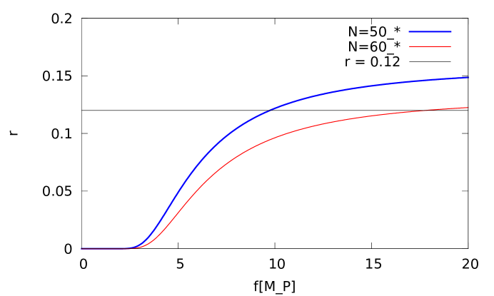
Figure 1: The scalar-to-tensor ratio, $r$, as a function of $f$ for different values of $N_{\ast}$.

Figure 2: The spectral index, $n_{s}$, as a function of $f$ for different values of $N_{\ast}$.

The power spectrum of the slow-roll inflation is given by

$$P_{\zeta}\simeq\frac{H^{2}}{8\pi^{2}M_{P}^{2}\epsilon_{V}}\,.$$ (2.16)

This should be compared with the observed value $P_{\zeta}(k_{\ast})=2.2\times 10^{-9}$ [1]. It determines the Hubble scale, $H_{\ast}$, when the pivot scale exited the horizon, and thus the energy density at that time, $\rho_{\ast}\simeq 3M_{P}^{2}H_{\ast}^{2}$, as a function of $f$ and $N_{\ast}$. Its dependence on $f$ and $N_{\ast}$ is mild, and we obtain $\rho_{\ast}\simeq 10^{16}$ GeV, see Fig. 3.

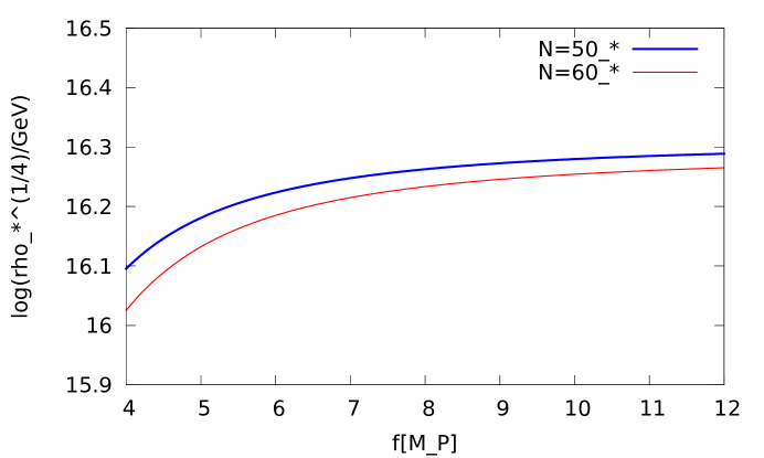
Figure 3: The energy density, $\rho_{\ast}$, as a function of $f$ for different values of $N_{\ast}$.

On the other hand, from the Friedman equation for spatially flat Universe in the slow-roll approximation,

$$3H^{2}M_{P}^{2}=\rho\simeq V(\phi)\,,$$ (2.17)

we obtain

$$P_{\zeta}(k_{\ast}) \simeq \frac{V(\phi_{\ast})}{24\pi^{2}M_{P}^{4}\epsilon_{V\ast}}$$ (2.18)

$$= \frac{c_{0}}{2\pi^{2}}\frac{1}{(2\pi L_{5})^{4}}\left[1-\cos\left(\frac{\phi_{\ast}}{f}\right)\right]\frac{1}{24\pi^{2}M_{P}^{4}\epsilon_{V\ast}}$$

$$= \frac{c_{0}}{2\pi^{2}}\frac{1}{(2\pi\ell_{5})^{6}}\left[1-\cos\left(\frac{\phi(f,N_{\ast})}{f}\right)\right]\frac{1}{24\pi^{2}\epsilon_{V}(\phi(f,N_{\ast}))}\,.$$

In the last line we have made it explicit that $\phi$ and $\epsilon_{V}$ are functions of $f$ and $N$. Thus given $\ell_{5}$, $f$ and $N_{\ast}$, $c_{0}$ is determined from the observed value $P_{\zeta}(k_{\ast})=2.2\times 10^{-9}$ by (2.18). The behaviour of $c_{0}$ as a function of $\ell_{5}$ is plotted in Fig. 4. We observe that $c_{0}$ grows as $\ell_{5}^{6}$. Also, $c_{0}$ grows rapidly with $f$, as seen in Fig. 5.

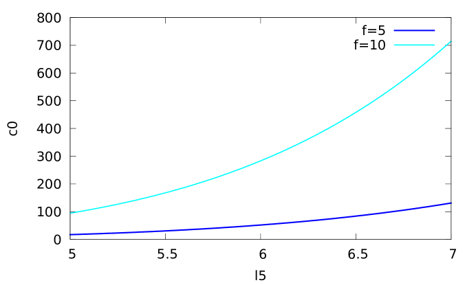
Figure 4: The behaviour of $c_{0}$ as a function of $\ell_{5}$ for $N_{\ast}=50$ at different values of $f$.

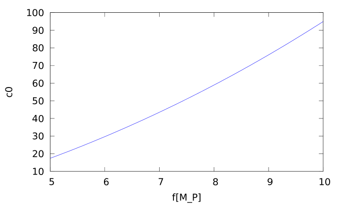
Figure 5: The behaviour of $c_{0}$ as a function of $f$ for $N_{\ast}=50$ and $\ell_{5}=5$.

Since each field charged under $U(1)_{B-L}$ with mass $\lesssim L_{5}^{-1}$ makes an ${\cal O}(1)$ contribution to $c_{0}$, if it is much larger than unity it may not be natural. Therefore we regard smaller values of $\ell_{5}$ and $f$, viz. $\ell_{5}\simeq 5$ and $f\simeq 5$, as preferred in our scenario here. With the independent parameters fixed, we then have $g_{4}\simeq 10^{-3}$ and $L_{5}^{-1}\simeq 9\times 10^{16}$ GeV from (2.11) and (2.9). The value of the $U(1)_{B-L}$ gauge coupling is an important input to our $U(1)_{B-L}$ extension of the SM, which we discuss next.

3 $U(1)_{B-L}$ extension of the Standard Model

There are several possibilities for the $U(1)_{B-L}$ extension of the SM, particularly with regards to the charge assignment of the scalar field that would break the $U(1)_{B-L}$ symmetry. Table 1 lists the particle content and the charge assignments of the particular $U(1)_{B-L}$ extension of the SM we consider here.

	$SU(3)_{c}$	$SU(2)_{L}$	$U(1)_{Y}$	$U(1)_{B-L}$
$q_{L}^{i}$	${\bf 3}$	${\bf 2}$	$+1/6$	$+1/3$
$u_{R}^{i}$	${\bf 3}$	${\bf 1}$	$+2/3$	$+1/3$
$d_{R}^{i}$	${\bf 3}$	${\bf 1}$	$-1/3$	$+1/3$
$\ell_{L}^{i}$	${\bf 1}$	${\bf 2}$	$-1/2$	$-1$
$\nu_{R}^{i}$	${\bf 1}$	${\bf 1}$	$0$	$-1$
$e_{R}^{i}$	${\bf 1}$	${\bf 1}$	$-1$	$-1$
$H$	${\bf 1}$	${\bf 2}$	$-1/2$	$0$
$\Sigma$	${\bf 1}$	${\bf 1}$	$0$	$+2$

Table 1: Particle contents and charge assignment. The index $i=1,2,3$ labels the generation.

In our set-up, we envisage all the SM particles and the right-handed neutrinos living on a four-dimensional brane, while the $U(1)_{B-L}$ gauge fields, $A_{M}$, and a complex scalar, $\Sigma$, responsible for the eventual $U(1)_{B-L}$breaking living in the five-dimensional bulk. In string theory this set-up may be realized, for example, when the SM fields and the right-handed neutrinos live on a (3+1)-dimensional D-brane localised in the extra dimension, while the bulk fields arise from higher dimensional D-branes.

The potential for the scalar sector renormalizable in four dimensions is given by

$$V(H,\Sigma)=\mu_{H}^{2}H^{\dagger}H+\mu_{\Sigma}^{2}\Sigma_{0}^{\ast}\Sigma_{0}+\frac{\lambda_{1}}{2}(H^{\dagger}H)^{2}+\frac{\lambda_{2}}{2}(\Sigma_{0}^{\ast}\Sigma_{0})^{2}+\lambda_{3}H^{\dagger}H\Sigma_{0}^{\ast}\Sigma_{0}\,.$$ (3.1)

Here, $\Sigma_{0}$ is the zero-mode of $\Sigma$ in the fifth direction. After spontaneous symmetry breaking, the scalar fields acquire vacuum expectation values (VEVs), and we can write

$$H=\frac{1}{\sqrt{2}}\begin{pmatrix}0\\ v_{H}+h\end{pmatrix},\qquad\Sigma_{0}=\frac{v_{\Sigma}+s}{\sqrt{2}}\,,$$ (3.2)

where $h$ and $s$ are excitations about the minimum, which is given by

$$\frac{v_{H}^{2}}{2}=\frac{-\mu_{H}^{2}\lambda_{2}+\mu_{\Sigma}^{2}\lambda_{3}}{\lambda_{1}\lambda_{2}-\lambda_{3}^{2}}\,,\qquad\frac{v_{\Sigma}^{2}}{2}=\frac{-\mu_{\Sigma}^{2}\lambda_{1}+\mu_{H}^{2}\lambda_{3}}{\lambda_{1}\lambda_{2}-\lambda_{3}^{2}}\,.$$ (3.3)

Note that the $W$ boson mass fixes $v_{H}=246$ GeV. In terms of $h$ and $s$, the quadratic part of the potential is given by

$$V^{(2)}=\frac{1}{2}\,\eta^{\intercal}M_{0}^{2}\,\eta\,,\quad\eta=\begin{pmatrix}h\\ s\end{pmatrix},$$ (3.4)

where

$$M_{0}^{2}=\begin{pmatrix}\lambda_{1}v_{H}^{2}&\lambda_{3}v_{H}v_{\Sigma}\\ \lambda_{3}v_{H}v_{\Sigma}&\lambda_{2}v_{\Sigma}^{2}\end{pmatrix},$$ (3.5)

is the tree-level mass-squared matrix for $h$ and $s$, and we have used the minimization condition for the potential. Diagonalizing, the physical mass eigenstates are defined by

$$\begin{pmatrix}h\\ s\end{pmatrix}=\begin{pmatrix}\cos\alpha&\sin\alpha\\ -\sin\alpha&\cos\alpha\end{pmatrix}\begin{pmatrix}h_{1}\\ h_{2}\end{pmatrix},$$ (3.6)

with the mixing angle given by

$$\tan 2\alpha=\frac{2\lambda_{3}v_{h}v_{s}}{\lambda_{2}v_{s}^{2}-\lambda_{1}v_{h}^{2}}\,.$$ (3.7)

The masses of the physical states are then given by

$$m_{h_{1,2}}^{2}=\frac{1}{2}\left\{\lambda_{1}v_{H}^{2}+\lambda_{2}v_{\Sigma}^{2}\mp\sqrt{(\lambda_{1}v_{H}^{2}-\lambda_{2}v_{\Sigma}^{2})^{2}+4\lambda_{3}^{2}v_{H}^{2}v_{\Sigma}^{2}}\right\}\,.$$ (3.8)

For $|\lambda_{3}|\ll 1$ and $|v_{H}/v_{\Sigma}|\ll 1$, we can expand the square root and obtain

$$m_{h_{1,2}}^{2}=\lambda_{1,2}v_{H,\Sigma}^{2}\mp\frac{\lambda_{3}^{2}}{\lambda_{2}}v_{H}^{2}+\lambda_{3}^{2}v_{H}^{2}\,\mathcal{O}\!\left(\frac{v_{H}^{2}}{v_{\Sigma}^{2}}\right)\,.$$ (3.9)

Assuming no coupling between the Higgs $H$ and the scalar $\Sigma_{0}$ at tree level, the mixing term $H^{\dagger}H\Sigma_{0}^{\ast}\Sigma_{0}$ is induced at one-loop level [13] through interactions with neutrinos responsible for the seesaw mechanism [14, 15, 16, 17]:

$$\mathcal{L}\supset-Y_{D}^{ij}\,\overline{\nu_{R}^{i}}\,H^{\dagger}\,l_{L}^{j}-\frac{1}{2}\,Y_{N}^{ij}\,\overline{\nu_{R}^{ic}}\,\nu_{R}^{j}\,\Sigma_{0}+\mathrm{h.c.}\,.$$ (3.10)

Fig. 6 displays the particular one-loop graph.

Figure 6: One-loop diagram which contributes to the mixing term $H^{\dagger}H\Sigma_{0}^{\ast}\Sigma_{0}$ through the right-handed neutrinos.

After $U(1)_{B-L}$ symmetry breaking, the mixing term contributes to the Higgs mass is estimated as

$$\delta m_{H}^{2}\sim\frac{Y_{D}^{2}Y_{N}^{2}}{(4\pi)^{2}}\frac{v_{\Sigma}^{2}}{2}\sim\frac{m_{\nu}M_{N}^{3}}{(4\pi)^{2}v_{H}^{2}}\,,$$ (3.11)

where we have used the seesaw formula $m_{\nu}\sim Y_{D}^{2}v_{H}^{2}/M_{N}$ with $M_{N}=Y_{N}v_{\Sigma}/\sqrt{2}$ being the mass of the right-handed neutrino. Given the observation of the Higgs boson with mass $126$ GeV at the LHC [18, 19, 20], we should have $\sqrt{|\delta m_{H}^{2}|}\lesssim 100$ GeV if naturalness is a criterion. Thus if we take $m_{\nu}\sim 0.1$ eV, we have $M_{N}\lesssim 10^{7}$ GeV from (3.11) and hence $v_{\Sigma}\lesssim 10^{7}/Y_{N}$ GeV. This translates to an upper bound on the mixing coupling

$$|\lambda_{3}|\sim\frac{Y_{D}^{2}Y_{N}^{2}}{(4\pi)^{2}}\sim\frac{m_{\nu}M_{N}}{(4\pi)^{2}v_{H}^{2}}Y_{N}^{2}\lesssim 10^{-10}\,Y_{N}^{2}\,.$$ (3.12)

Assuming $Y_{N}\simeq{\cal O}(1)$, the mass of the physical $U(1)_{B-L}$ gauge boson is estimated as

$$m_{Z^{\prime}}\sim g_{4}v_{\Sigma}\lesssim{\cal O}(10^{4})\,\mathrm{GeV}\,.$$ (3.13)

From collider experiments, one has $m_{Z^{\prime}}\geq g_{4}\times(6\,\mathrm{TeV})$ for a $U(1)_{B-L}$ $Z^{\prime}$ boson [21]. Since $g_{4}\lesssim 10^{-3}$, there are no stringent bounds on $m_{Z^{\prime}}$.

4 The inflaton decay

The coupling between the inflaton and the SM particles is crucial at the time of reheating. Let us first consider the following $\mathbb{Z}_{2}$ transformation:

$$x^{5}\rightarrow-x^{5},\quad A_{5}\rightarrow-A_{5}\,.$$ (4.1)

We choose the origin of the $x^{5}$ coordinate to be where the brane is localised. We assume there are no other fields with $\mathbb{Z}_{2}$-odd charges under (4.1) that are lighter than $A_{5}$. Then if this $\mathbb{Z}_{2}$ transformation is an exact symmetry, the inflaton is absolutely stable. This will be a problem, however, since then the Universe could not be heated to bring forth the standard hot big bang cosmology. We therefore introduce a five-dimensional Chern-Simons term, which breaks the $\mathbb{Z}_{2}$ symmetry:

$$S_{CS}=\frac{k}{48\pi^{3}}\int\,{\cal A}{\cal F}^{2},$$ (4.2)

where ${\cal A}={\cal A}_{M}dx^{M}$, ${\cal F}=\frac{1}{2}{\cal F}_{MN}dx^{M}dx^{N}$, and $k$ is some integer. Here, ${\cal A}_{M}$ is the $U(1)_{B-L}$ gauge field with mass dimension one, which is related to the canonically normalized fields by

$$A_{M}^{(5)} = \frac{1}{g_{5}}{\cal A}_{M}\,,$$ (4.3)

$$A_{\mu} = \frac{1}{g_{4}}{\cal A}_{\mu\,0}\,,\quad\phi=\frac{1}{g_{4}}{\cal A}_{5\,0}\,,$$ (4.4)

where $A_{M}^{(5)}$ is the $U(1)_{B-L}$ gauge field canonically normalized in five dimensions, $A_{\mu}$ that in four dimensions, and ${\cal A}_{M\,0}$ the zero-mode of ${\cal A}_{M}$ in five dimensions.

The four-dimensional interaction of the zero-modes following from (4.2) is

$$\frac{k}{48\pi^{3}}\int d^{4}x\,(2\pi L)\frac{3}{4}\epsilon^{\mu\nu\rho\sigma}{\cal A}_{5\,0}{\cal F}_{\mu\nu\,0}{{\cal F}}_{\rho\sigma\,0} = \frac{k}{16\pi^{2}}\int d^{4}x\,\frac{\phi}{2\pi f}{\cal F}_{\mu\nu\,0}\tilde{{\cal F}}_{\,0}^{\mu\nu}$$ (4.5)

$$= g_{4}^{2}\frac{k}{16\pi^{2}}\int d^{4}x\,\frac{\phi}{2\pi f}F_{\mu\nu}\tilde{F}^{\mu\nu}.$$

Here the subscript $0$ denotes that they are (made from) zero-modes in the fifth direction.

The coupling (4.5) gives the dominant contribution to the decay width at the tree level:

$$\Gamma_{\phi\rightarrow AA}\simeq\frac{g_{4}^{4}}{16\pi}\left(\frac{k}{32\pi^{3}}\right)^{2}\frac{m_{\phi}^{3}}{f^{2}}\,,$$ (4.6)

where $m_{\phi}$ is the mass of the inflaton. As we have seen, $c_{0}$ is determined by (2.18) once $f$ and $g_{4}$ are given. This then determines $m_{\phi}$:

$$\frac{m_{\phi}^{2}}{2}=\frac{V_{0}}{4f^{2}}=\frac{1}{4f^{2}}\frac{c_{0}}{\pi^{2}}\frac{1}{(2\pi L_{5})^{4}}=\frac{c_{0}g_{4}^{4}f^{2}}{4\pi^{2}}\,.$$ (4.7)

The $U(1)_{B-L}$ gauge bosons decay to SM particles via the minimal couplings. As this proceeds much faster than the inflaton decay, the reheating temperature is governed by the inflaton decay width (4.6). It is estimated as

$$T_{R} = \left(\frac{90}{\pi^{2}g_{\star}(T_{R})}\right)^{1/4}\sqrt{\Gamma M_{P}}\simeq\left(\frac{90}{g_{\star}(T_{R})}\right)^{1/4}\frac{g_{4}^{2}}{4\pi}\frac{|k|}{32\pi^{3}}\sqrt{\frac{m_{\phi}^{3}M_{P}}{f^{2}}}$$ (4.8)

$$\simeq |k|\times 1\,\,\mathrm{GeV}\,,$$

where in the last line, we have used the preferred values $f\simeq 5M_{P}$ and $\ell_{5}\simeq 5$, which gives $m_{\phi}\simeq 10^{13}$ GeV. The factor $g_{\star}(T)$ is the effective relativistic degrees of freedom at temperature $T$. For $T_{R}\simeq 1\sim 10$ GeV, $g_{\star}(T_{R})\simeq 60\sim 90$. From (4.8), the reheating temperature is much smaller than the $U(1)_{B-L}$ breaking scale given by $v_{\Sigma}\simeq{\cal O}(10^{7})$ GeV, when $k$ is ${\cal O}(1-10)$. Comparing (4.8) with the standard estimate of the number of e-folds [22]:

$$N_{\ast}\simeq 49+\frac{2}{3}\ln\left(\frac{\rho_{\ast}^{1/4}}{10^{16}\,\mbox{GeV}}\right)+\frac{1}{3}\ln\left(\frac{T_{R}}{1\,\mbox{GeV}}\right)\,,$$ (4.9)

we observe that $N_{\ast}\simeq 50$ is natural in our model, as advertised earlier.

5 Summary and Discussions

In this letter, we have studied the interrelation between cosmology and particle physics in $U(1)_{B-L}$ extra-natural inflation with a gauged $U(1)_{B-L}$ extension of the SM localised on a brane. The cosmological observation constrains the value of the $U(1)_{B-L}$ gauge coupling to $g_{4}\lesssim 10^{-3}$, which in turn constrains the particle physics scenario at high energy assuming naturalness. On the other hand, with SM particles localised on a brane, allowed interaction between the inflaton and the SM particles are restricted. Together with the value of $g_{4}$, the decay width of the inflaton and the reheating temperature are determined.

By tuning of a few parameters or with some slight extension, our model may also be able to explain other cosmological observations such as the Baryon number asymmetry of the Universe and the dark matter abundance. Indeed, the right-handed neutrinos could play a role in the former through the leptogenesis. They are also dark matter candidates. Another possible dark matter candidate, which may be included in our model, is a light scalar field odd under the reflection of the extra dimension (4.1). These merit further investigations.

Our main purpose in this letter is to present an example in which the relation between the BSM physics and the inflation physics are specified, and theoretical and observational constraints on one side constrains the other. We discussed one example here, but there can be several other possibilities, even within gauged $U(1)_{B-L}$ extensions of the SM. For instance, one may put some of the SM fields in the bulk. It will be interesting to explore those related scenarios.

Acknowledgments

The authors would like to thank Chong-Sun Chu, Satoshi Iso, Hiroshi Isono, Yoji Koyama and Chia-Min Lin for stimulating discussions. KF is grateful to his former institutions, National Center for Theoretical Sciences and the Department of Physics, National Tsing-Hua University, where part of this work has been done.

References

- [1] Planck Collaboration Collaboration, P. Ade et al., “Planck 2013 results. XXII. Constraints on inflation,” arXiv:1303.5082 [astro-ph.CO].
- [2] D. H. Lyth, “What would we learn by detecting a gravitational wave signal in the cosmic microwave background anisotropy?,” Phys.Rev.Lett. 78 (1997) 1861–1863, arXiv:hep-ph/9606387 [hep-ph].
- [3] N. Arkani-Hamed, H.-C. Cheng, P. Creminelli, and L. Randall, “Extra natural inflation,” Phys.Rev.Lett. 90 (2003) 221302, arXiv:hep-th/0301218 [hep-th].
- [4] D. E. Kaplan and N. J. Weiner, “Little inflatons and gauge inflation,” JCAP 0402 (2004) 005, arXiv:hep-ph/0302014 [hep-ph].
- [5] R. N. Mohapatra and R. Marshak, “Local B-L Symmetry of Electroweak Interactions, Majorana Neutrinos and Neutron Oscillations,” Phys.Rev.Lett. 44 (1980) 1316–1319.
- [6] R. Marshak and R. N. Mohapatra, “Quark - Lepton Symmetry and B-L as the U(1) Generator of the Electroweak Symmetry Group,” Phys.Lett. B91 (1980) 222–224.
- [7] C. Wetterich, “Neutrino Masses and the Scale of B-L Violation,” Nucl.Phys. B187 (1981) 343.
- [8] A. Masiero, J. Nieves, and T. Yanagida, “ Violating Proton Decay and Late Cosmological Baryon Production,” Phys.Lett. B116 (1982) 11.
- [9] T. Inami, Y. Koyama, C. Lim, and S. Minakami, “Higgs-Inflaton Potential in 5D Super Yang-Mills Theory,” Prog.Theor.Phys. 122 (2009) 543–551, arXiv:0903.3637 [hep-th].
- [10] T. Inami, Y. Koyama, C.-M. Lin, and S. Minakami, “Inflaton versus Curvaton in Higher Dimensional Gauge Theories,” Prog.Theor.Phys. 125 (2011) 345–358, arXiv:1004.5477 [hep-ph].
- [11] K. Freese, J. A. Frieman, and A. V. Olinto, “Natural inflation with pseudo - Nambu-Goldstone bosons,” Phys.Rev.Lett. 65 (1990) 3233–3236.
- [12] H. Hatanaka, T. Inami, and C. Lim, “The Gauge hierarchy problem and higher dimensional gauge theories,” Mod.Phys.Lett. A13 (1998) 2601–2612, arXiv:hep-th/9805067 [hep-th].
- [13] S. Iso, N. Okada, and Y. Orikasa, “Classically conformal extended Standard Model,” Phys.Lett. B676 (2009) 81–87, arXiv:0902.4050 [hep-ph].
- [14] P. Minkowski, “mu e gamma at a Rate of One Out of 1-Billion Muon Decays?,” Phys.Lett. B67 (1977) 421.
- [15] T. Yanagida, “HORIZONTAL SYMMETRY AND MASSES OF NEUTRINOS,” Conf.Proc. C7902131 (1979) 95–99.
- [16] M. Gell-Mann, P. Ramond, and R. Slansky, “COMPLEX SPINORS AND UNIFIED THEORIES,” Conf.Proc. C790927 (1979) 315–321.
- [17] S. Glashow, “THE FUTURE OF ELEMENTARY PARTICLE PHYSICS,” NATO Adv.Study Inst.Ser.B Phys. 59 (1980) 687.
- [18] ATLAS Collaboration Collaboration, G. Aad et al., “Measurements of Higgs boson production and couplings in diboson final states with the ATLAS detector at the LHC,” Phys.Lett. B726 (2013) 88–119, arXiv:1307.1427 [hep-ex].
- [19] ATLAS Collaboration Collaboration, G. Aad et al., “Evidence for the spin-0 nature of the Higgs boson using ATLAS data,” Phys.Lett. B726 (2013) 120–144, arXiv:1307.1432 [hep-ex].
- [20] CMS Collaboration Collaboration, “Properties of the Higgs-like boson in the decay H to ZZ to 4l in pp collisions at sqrt s =7 and 8 TeV,”.
- [21] M. S. Carena, A. Daleo, B. A. Dobrescu, and T. M. Tait, “ gauge bosons at the Tevatron,” Phys.Rev. D70 (2004) 093009, arXiv:hep-ph/0408098 [hep-ph].
- [22] D. H. Lyth and A. R. Liddle, “The primordial density perturbation: Cosmology, inflation and the origin of structure,” Cambridge Univ. Press (2009) .