A Greedy Algorithm for Optimally Pipelining a Reduction

Abstract

Collective communications are ubiquitous in parallel applications. We present two new algorithms for performing a reduction. The operation associated with our reduction needs to be associative and commutative. The two algorithms are developed under two different communication models (unidirectional and bidirectional). Both algorithms use a greedy scheduling scheme. For a unidirectional, fully connected network, we prove that our greedy algorithm is optimal when some realistic assumptions are respected. Previous algorithms fit the same assumptions and are only appropriate for some given configurations. Our algorithm is optimal for all configurations. We note that there are some configuration where our greedy algorithm significantly outperform any existing algorithms. This result represents a contribution to the state-of-the art. For a bidirectional, fully connected network, we present a different greedy algorithm. We verify by experimental simulations that our algorithm matches the time complexity of an optimal broadcast (with addition of the computation). Beside reversing an optimal broadcast algorithm, the greedy algorithm is the first known reduction algorithm to experimentally attain this time complexity. Simulations show that this greedy algorithm performs well in practice, outperforming any state-of-the-art reduction algorithms. Positive experiments on a parallel distributed machine are also presented.

I Introduction

Applications relying on parallel distributed communication require the use of collective communications. In this paper, we focus on the reduction operation (MPI_Reduce) in which each process holds a piece of data and these pieces of data need to be combined using an associative operation to form the results on the root process. We present two new algorithms for performing a reduction. The operation associated with our reduction needs to be associative and commutative. The two algorithms are developed under two different communication models (unidirectional and bidirectional). Both algorithms use a greedy scheduling scheme.

Collective communications like reduction can often be the bottleneck of massively parallel application codes, therefore optimizing collective communications can greatly improve the performance of such application codes. The performance of a reduction algorithm is highly dependent on the machine parameters (e.g., network topology) and the underlying architecture; this makes the systematic optimization of a collective communication for a given machine a real challenge. For a unidirectional, fully connected network, we prove that our greedy algorithm is optimal when some realistic assumptions are respected. Previous algorithms fit the same assumptions and are only appropriate for some given configurations. Our algorithm is optimal for all configurations. We note that there are some configuration where our greedy algorithm significantly outperform any existing algorithms. This result represents a contribution to the state-of-the art. For a bidirectional, fully connected network, we present a different greedy algorithm. We verify by experimental simulations that our algorithm matches the time complexity of an optimal broadcast (with addition of the computation). Beside reversing an optimal broadcast algorithm, the greedy algorithm is the first known reduction algorithm to experimentally attain this time complexity. Simulations show that this greedy algorithm performs well in practice, outperforming any state-of-the-art reduction algorithms. With respect to practical application, much work is still needed in term of auto-tuning and configuring for various architectures (nodes of multi-core, multi-port networks, etc.).

In the unidirectional context, we compared the greedy algorithm (uni-greedy) with three standard algorithms (binomial, pipeline, and binary) using a linear model to represent the point-to-point cost of communicating between processors. Unlike the standard algorithms, no closed-form expression exists for the completion time of the greedy algorithm; therefore, simulations are used to compare the algorithms. While we know that our algorithm is optimal in this context, these simulations indicate the performance gain of the new algorithm over classic ones. In particular, for mid-size messages, the new algorithm is about 50% faster than pipeline, binary tree, or binomial tree.

In the bidirectional context, we again compare the greedy algorithm (bi-greedy) with the three standard algorithms as well as a reduce-scatter/gather (butterfly) algorithm. For the standard algorithms we see similar results as the unidirectional case. The butterfly algorithm performs well for mid-size messages, but has poor asymptotic behavior.

In the experimental context, we have implemented the binomial, pipeline, uni-greedy, and bi-greedy algorithms using OpenMPI version 1.4.3; all algorithms are implemented using point-to-point MPI functions: MPI_Send and MPI_Recv, or MPI_Sendrecv. Moreover, the OpenMPI library provides a state-of-the-art implementation for a reduction. We also, compare with an implementation of the butterfly algorithm. Numerical comparisons of the greedy algorithm to OpenMPI’s built in function MPI_Reduce as well as the binomial and pipeline algorithms show the greedy algorithm is the best for medium size messages, confirming that the results found theoretically applies in our experimental context. However, the more simplistic algorithms (binomial and pipeline) perform better for small and large messages, respectively. Finally, the implementation of the butterfly algorithm exhibits similar results as in the theoretical context.

Finally, the idea of unequal segmentation is considered. Typically, when a message is split into segments during a reduction operation, the segments are assumed to be of equal size. We investigate if the greedy and pipeline algorithms can be improved by allowing for segments to have unequal sizes. It turns out that, for some parameter values, the greedy algorithm (in a unidirectional system) was optimized by unequal segmentations. This indicates that removing the equal segmentation assumption from our theory can lead to better algorithms. However, the gains obtained were marginal. We also note that the pipeline algorithm was always optimized by equal segmentation.

II Model

Unidirectional and bidirectional systems are two ways to describe how processors are allowed to communicate with each other. In a unidirectional system, a processor can only send a message or receive a message at a given time, but not both. A bidirectional system assumes that at a given time a processor may receive a message from a processor and send a message to another (potentially different) processor simultaneously. We assume an unidirectional system for the initial sections and optimality proof (Sections IV and V). In Section VI we adapt the algorithm to a bidirectional system.

The parallel system contains $p$ processors indexed from 0 to $p-1$. Additionally, we will assume the system is fully connected (every processor has a direct connection to all other processors) and homogeneous. These assumptions are not verified in practice on current architecture, however they represent a standard theoretical framework and our experiments indicate that they are valid enough in practice to develop useful algorithms.

A linear model (Hockney [1]) is used to represent the cost of a point-to-point communication. The time required for each communication is given by $\alpha+\beta m$, where $\alpha$ is the latency (start up), $\beta$ is the inverse bandwidth (time to send one element of the message), and $m$ is the size of the message. Since we are performing a reduction, computations are also involved so we will also assume the time for computation follows a linear model and is given by $\gamma m$, where $\gamma$ is the computation time for one element of the message. We will investigate the theoretical case when $\gamma=0$ (i.e., very fast processing units) as well as for nonzero $\gamma$. Furthermore, we will assume that communication and computation can not overlap.

To achieve better performance the messages can be split into $q$ segments of size $s_{1},\dots,s_{q}$. In Section V we show the greedy algorithm is optimal for any segmentation. To obtain the best performance of a given algorithm an optimal segmentation is determined. In Section V-B we restrict the optimization to equi-segmentation ($s_{i}=s,\;\forall\;i$), except the last segment may possibly be smaller.

III Collective Communications and Related Work

A collective communication operation is an operation on data distributed between a set of processors (a collective). Examples of collective communications are broadcast, reduce (all-to-one), reduce (all-to-all), scatter, and gather.
Broadcast: Data on one processor (the root) is distributed to the other processors in the collective.
Reduce: Each processor in a collective has data that is combined entry-wise and the result is stored on the root processor.
All Reduce: Same as reduce except that all processors in the collective contain a copy of the result.
Scatter: Data that is on the root processor is split into pieces and the pieces are distributed between the processors in the collective. The result is each processor (including the root processor) contains a piece of the original data.
Gather: The reverse operation of a scatter.

Optimizing the reduction operation is closely related to optimization of the broadcast operation. Any broadcast algorithm can be reversed to perform a reduction. Bar-Noy et al. [2] and Träff and Ripke [3] both provide algorithms that produce an optimal broadcast schedule for a bidirectional system. Here the messages are split into segments and the segments are broadcast in rounds. In both cases the optimality is in the sense that the algorithm meets the lower bound on the number of communication rounds. For the theoretical case when $\gamma=0$, reversing an optimal broadcast will provide an optimal reduction. However, for $\gamma\neq 0$ this is no longer valid as an optimal schedule will most like take into account the computation.

Rabenseifner [4] provides a reduce-scatter/gather algorithm (butterfly) which provides optimal load balancing to minimize the computation. Rabenseifner does not predefine a segmentation of the message, but rather uses the techniques recursive-halving and recursive-doubling. The algorithm is done in two phases. In the first phase the message is repeatedly halved in size and exchanged among processes. At the end of the first phase the final result is distributed among all the processors. This phase is know as a reduce-scatter. The second phase gathers the results recursively doubling the size of the message. In [5] Rabenseifner and Träff improve on the algorithm for non-power of two number of processors.

Sanders et al. [6] introduce an algorithm to schedule to a reduction (or broadcast) using two binary trees. The authors notice that two binary trees could be use simultaneously and effectively reduce the bandwidth by a factor of two from a single binary tree. The time complexity approaches the lower bound for large messages. However, for small messages the latency term is twice larger than optimal. Also, the time complexity is never better than that of a reverse-optimal broadcast.

Other models have been used to describe more complex machine architectures. Heterogeneous networks, where processor characteristics are composed of different communication and computation rates, have been considered. Beaumont et al. [7, 8] consider optimizing a broadcast and Legrand et al. [9] consider optimizing scatter and reduce. In these papers, the problem is formulated as a linear program and solved to maximize the throughput (number of messages broadcasting per time unit). Also, higher dimensional systems have also been considered [10]. Here a processor can communicate with more than one processor at a time.

The machine parameters and architecture vary between machines and one algorithm may perform better on one machine versus another. Accurately determining machine parameters can be a difficult task. In practice, auto-tuning for each machine is required to obtain a well-performing algorithm. Vadhiyar et al. [11] discuss how to experimentally determine the optimal algorithm. Pjesivac-Grbović et al. [12] compare various models that can be used to auto-tune a machine. These models are more complex than the Hockney model and can provide a more accurate model for the communication cost. However, a linear model provides a good bases for theoretically comparing algorithms. Other models, such as LogP, LogGP, and PLogP, each provided useful information to help auto-tune a machine.

IV Standard Algorithms

Before introducing the greedy algorithms it is helpful to review three standard algorithms (binomial, pipeline, and binary).

Since we are using a unidirectional system, we will call a processor either a sending processor or a receiving processor. Sending and receiving processors are paired together to perform a reduction. After a receiving processor receives a segment it will combine its segment with the segment received. After a processor sends a segment it is said to be reduced for that segment. For the reduction to be completed each processor (except the root) must be reduced for each segment. The three algorithms are described below.

Binomial

At a given time suppose there are $n$ processors left to be reduced for a message, then $\lfloor n/2\rfloor$ processors are assigned as sending processors and $\lfloor n/2\rfloor$ are assigned as receiving processors. Afterwards there will be $\lceil n/2\rceil$ processors left for reduction and the process is repeat until $n=1$. Segmenting the message would only increase the latency of the communication time since all processors must be finished before the next segment can be started. Therefore, we do not consider segmentation.

Pipeline

At a given time suppose that processors $k+1$ to $p-1$ have been reduced for segment $s_{i}$. Processor $k$ is assigned as a sending processor for segment $s_{i}$ and processor $k-1$ is assigned as a receiving processor for segment $s_{i}$.

Binary

At a given time suppose there are $2^{n}-1$ processors left to be reduced for segment $s_{i}$, then $2^{n-1}$ processors are assigned as sending processors and $2^{n-2}$ processors are assigned as receiving processors. If $p\neq 2^{n}-1$ for some $n$, then the initial step in the algorithm reduces the “extra” processors so that in the next step there is $2^{n}-1$, for some $n$, processors left for reduction. Since there are twice as many sending processors as receiving processors, two processors will send to the same receiving processor and the time for one step in the binary algorithm is $2(\alpha+\beta s+\gamma s)$.

IV-A Lower bounds and optimality of the segment size $s$.

Binomial	Time	$\lceil log_{2}p\rceil(\alpha+\beta m+\gamma m)$
Pipeline	Time	$(p-1)(\alpha+\beta s+\gamma s)+2(q-1)(\alpha+\beta s+\gamma s)$
	$s_{opt}$	$\left(\dfrac{2m\alpha}{(p-3)(\beta+\gamma)}\right)^{1/2}$
	$T_{opt}$	$\left[\left((p-3)\alpha\right)^{1/2}+\left(2m(\beta+\gamma)\right)^{1/2}\right]^{2}$
Binary	Time	$2\left(\lceil log_{2}(p+1)\rceil-1\right)(\alpha+\beta s+\gamma s)+4(q-1)(\alpha+\beta s+\gamma s)$
	$s_{opt}$	$\left(\dfrac{2m\alpha}{(N-3)(\beta+\gamma)}\right)^{1/2}$
	$T_{opt}$	$2\left[\left((N-3)\alpha\right)^{1/2}+\left(2m(\beta+\gamma)\right)^{1/2}\right]^{2}$

TABLE I: Time analysis for standard algorithms in a unidirectional system, where $N=\lceil\log_{2}(p+1)\rceil$, $s_{opt}$ is the optimal equi-segment size, and $T_{opt}$ is the time for the algorithm at $s_{opt}$. Formulae are valid for $p>3$.

	Latency	Bandwidth	Computation
Reduce	$\lceil log_{2}p\rceil\alpha$	$2m\beta$	$\frac{p-1}{p}m\gamma$
Binomial	$\lceil\log_{2}p\rceil\alpha$	$\lceil\log_{2}p\rceil m\beta$	$\lceil\log_{2}p\rceil m\gamma$
Pipeline	$(p-1)\alpha$	$(p+2m-3)\beta$	$(p+2m-3)\gamma$
Binary	$2(N-1)\alpha$	$2(N+2m-3)\beta$	$2(N+2m-3)\gamma$

TABLE II: Lower bounds for each term in the time for a reduction as well as the lower bounds for each standard algorithm in a unidirectioanl, where $N=\lceil\log_{2}(p+1)\rceil$. Formulae are valid for $p>2$.

Given $p$, $\alpha$, $\beta$, $\gamma$, $m$, and $s$, the time for a reduction can be calculated for each algorithm. Using these formulae the optimal segmentation size ($s_{opt}$) and optimal time ($T_{opt}$) can also be calculated. When calculating the optimal segmentation size we assume that the segments are of equal size. A summary of these values is given in Table I. It is unknown what the optimal segmentation would be if the segments are of unequal size. The formulae for time are upper bounds in the case when $m$ is not divisible by $s$. These formulae differ from the formulae that appear in  [3, 12] by a factor of 2 in the bandwidth term since the authors assume a bidirectional system. In a unidirectional system there is extra lag time.

To better understand the algorithms it is helpful to know the lower bounds for each term:$\alpha$, $\beta$, and $\gamma$. The lower bounds for any reduction algorithm as well as other collective communications are discussed in [13]. The following rationales are used to obtain the lower bounds.

Latency

Every processor in a collective has at least one message that must be communicated. At any time step, at most half of the remaining processors can send their messages to another processor to perform the reduction. This gives the lower bound $\lceil\log_{2}p\rceil\alpha$.

Bandwidth

Consider the case when $p=3$. Each processor must be involved in a communication for each element of the message. When two processors are involved in a communication the third processor is idle. Therefore, there must be two communications performed for each element of the message, which cannot occur simultaneously. This gives the lower bound $2m\beta$. For $p>3$, the lower bound holds since a message of the same size on more processors can not be communicated faster. $p=2$ is a special case with a bandwidth term of $m\beta$.

Communication

Each element of the message must be involved in $p-1$ computations. Distributing the computations evenly among all the processors gives the lower bound $\frac{p-1}{p}m\gamma$.

The lower bounds for the standard algorithms can be obtained using the following rationale. The latency term will be minimized when no segmentation is used ($q=1$), since any segmentation will only increase the number of time steps and hence increase the latency. The bandwidth and computation terms will be minimized when $s=1$, since this will maximize the time when multiple processors are working simultaneously. Table II shows the lower bounds for any reduction algorithm and the lower bounds for each of the standard algorithms.

Given machine parameters $\alpha$, $\beta$ and $\gamma$, one can select the algorithm that provides the best performance. In practice, the latency is much larger than the bandwidth $(\alpha\gg\beta)$. For small messages, $\alpha\gg\beta m$, the time for a reduction is dominated by the latency. The binomial algorithm minimizes the latency term and will provide the best performance for small messages. For large messages, $\alpha\ll\beta m$, the time for a reduction is dominated by the bandwidth. The pipeline algorithm provides the smallest bandwidth term and will therefore give the best performance for large messages. For medium size messages, the binary algorithm will provide the best performance. The binary algorithm has both qualities that give binomial and pipeline good lower bounds for latency and bandwidth, respectively, only differing by a factor of two.

The values of $m$ that are considered “small” and “large” depend on the machine parameters ($\alpha$, $\beta$, $\gamma$, and $p$). Figure 1 shows which algorithm is best for $\alpha=10$, $\beta=1$, $\gamma=0$ as a function of the number of processors $p$ and the message size $m$. Here we are assuming that there is no time required for the computation $(\gamma=0)$.

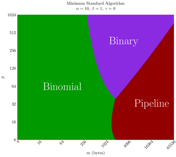
Figure 1: Regions where binomial or pipeline or binary is better in term of the number of processors ($p$) and the message size ($m$). For each algorithm, each $p$ and each $m$, the optimal segment size ($s_{opt}$) is obtained from the formulae given in Table I. The machine parameters are $\alpha=10$, $\beta=1$, $\gamma=0$ .

V A Greedy Algorithm for Unidirectional System

When a message is split into segments a reduction algorithm consists of scheduling $(p-1)q$ send/receive pairs (one for each segment of the non-root processors). For a segment $i$ of size $s_{i}$, the sending processor in a communication will be available after $t_{comm}(i)=\alpha+\beta s_{i}$, and the receiving processor will be available after $t_{comm}(i)+t_{comp}(i)$, where $t_{comp}=\gamma s_{i}$. We will add an extra requirement that segment $i$ must be reduced on a processor before that processor can be involved in a reduction for segment $j$, $j>i$. This requirement provides two benefits. First, since the schedule that is generated for a given number of processors and number of segments will vary, we must log the current state on each processor. With this requirement we only need a small array with a length equal to the number of processors. Second, if a processor has started but has not been reduced for multiple segments then each segments current result must be stored on the processor. This would require additional storage space on that processor.

Since we assume that each processor must reduce the segments in order, then a reduction can be scheduled considering one segment at a time. Let $I$ be a set of $n$ processors that remain to send a given segment (or for the root, receive the final message). Let $x_{i}$ be the time that processor $i$ completed its previous task. We define the state of these processors as

$$X^{(n)}=\{x_{i}|i\in I\}.$$

The state of the processors that have sent the segment is $S^{(n)}$. The permutation $P(X^{(n)})$ orders the elements of $X^{(n)}$ from smallest to largest. The time complexity of an algorithm is given by the final state of the root processor. A schedule for a send/receive pair is given by

$$(X^{(n-1)}_{k},S^{(n-1)}_{k})=\textmd{reduce}(X^{(n)}_{k},S^{(n)}_{k},a,b,t).$$

Processor $a$ sends segment $k$ to processor $b$ starting at time $t$. $X^{(n-1)}_{k}$ is the updated state of the processors that remain to send segment $k$ and $S^{(n-1)}_{k}$ is the state of the processors that have sent segment $k$. We will assume that successive send/receive pairs are scheduled in the order that the communications are started. This way the state of a processor that is not a memeber of the send/receive pair, but whose current state is less than $t$ is set equal to $t$.

Lemma 1.

$\textmd{reduce}(X^{(n)},S^{(n)},a,b,t)$, where $P(X^{(n)})=(x_{g_{1}},x_{g_{2}},\dots,x_{g_{n}})$, is a valid
send/receive pair if and only if

1. $x_{a}\leq t$ and $x_{b}\leq t$;

2. $a\neq 0$; and

3. $t\geq x_{g_{2}}$.

Proof.

(i) requires that processor $a$ and $b$ have completed their previous task before $t$. (ii) states that the root can never be a sending processor. And (i) implies (iii). ∎

A greedy algorithm is obtained by scheduling every send/receive pair using $t=x_{g_{2}}$ in Lemma 1. When a segment is done being scheduled then the final state of the processors are used as the initial state for the next segment. Algorithm 1 produces the unidirectional greedy (uni-greedy) schedule. A proof of optimality is given in Section V-A.

$X^{(p)}_{1}=\{0,\dots,0\}\;S^{(p)}_{1}=\emptyset$

for  $i=1$ to $q$  do

       for  $j=p$ downto $2$  do

             $P(X^{(j)}_{i})=(x_{g_{1}},x_{g_{2}},\dots x_{g_{j}})$

             $t=x_{g_{2}}$

             $(X^{(j-1)}_{i},S^{(j-1)}_{i})=\textmd{reduce}(X^{(j)}_{i},S^{(j)}_{i},g_{1},g_{2},t)$

            

      $X^{(p)}_{i+1}=X^{(1)}_{i}\bigcup S^{(1)}_{i}$

      

Algorithm 1 Uni-greedy Schedule

Figure 2: C code for the uni-greedy reduction algorithm. The algorithm assumes that MPI_Op is commutative (and associative as well, of course). The algorithm allocates two extra buffers of size segment size. The global variable global_s is the size of a segment and needs to be initialized (if possible “tuned”) in advance. The implementation is restricted to root being 0, MPI_Datatype being int, and MPI_Op being +. These restrictions are not a consequence of the algorithm and can be removed.

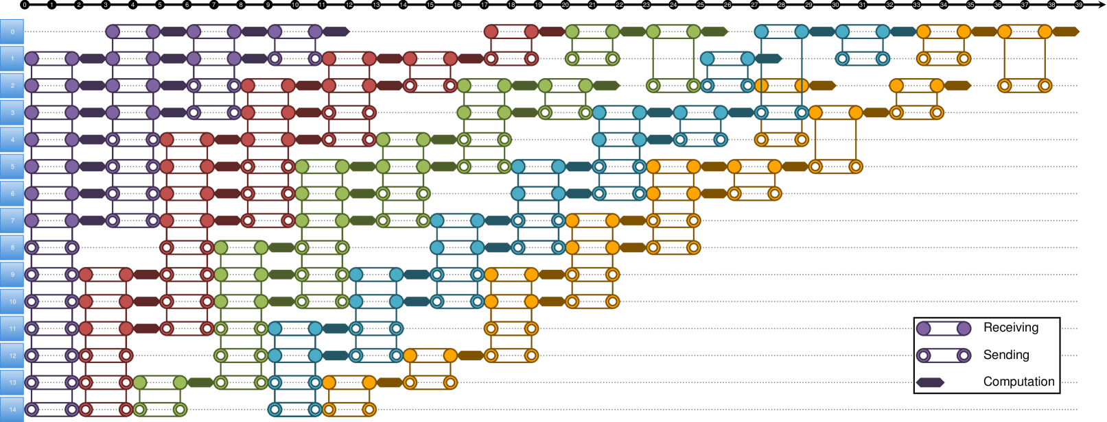
Figure 3: Uni-greedy algorithm for 15 processors and 5 equi-segments for $t_{comm}=2$ and $t_{comp}=1$. Each color represents a different segment. Filled in circles represent receiving processors, open circles represent sending processors, and hexagons represent computation.

We give the C code for the uni-greedy algorithm on the next page in Figure 2. In this code, we are able to generate the greedy schedule dynamically during the reduction rather than precomputing the schedule by Algorithm 1. The algorithm assumes that MPI_Op is commutative (and associative as well, of course). The algorithm allocates two extra buffers of size segment size. The variable s is the size of a segment and needs to be initialized (if possible “tuned”) in advance. The implementation is restricted to root being 0, MPI_Datatype being int, and MPI_Op being +. These restrictions are not a consequence of the algorithm and can be removed. In the next section we analyze the theoretical time for the greedy algorithm for various values of $\alpha$, $\beta$, and $\gamma$.

No closed-form expression for the time complexity of the uni-greedy algorithm exists like those given in Table I for the standard algorithms. Figure 3 gives an example for 15 processors and 5 equi-segments with $t_{comm}=2$ and $t_{comp}=1$. From time 12 to 15 provides an example where if we allowed segments to be reduced out of order then the uni-greedy algorithm would not be optimal. Without this restriction processor 8 could send segment 4 to processor 0 and the overall time complexity could be reduced by 1. We choose to omit the figure that shows the improvement.

V-A Proof of Optimality

In this section, we prove that the uni-greedy algorithm is optimal. The proof is a variation of the proof in [14]. Using the notation as in Lemma 1, we define

$$\textmd{optreduce}(X^{(n)})=\textmd{reduce}(X^{(n)},S^{(n)},g_{1},g_{2},x_{g_{2}}).$$

We also define the partial ordering on $\mathbb{R}^{n}$:

$$X\leq Y\iff x_{i}\leq y_{i},\;1\leq i\leq n.$$

Lemma 2.

Let $X\in\mathbb{R}^{n}$ and $Y\in\mathbb{R}^{n}$ be nondecreasing such that $X\leq Y$ and let $a\in\mathbb{R}$ and $b\in\mathbb{R}$ such that $a\leq b$. If $x_{k}\leq a\leq x_{k+1}$ and $y_{l}\leq b\leq y_{l+1}$, then

$$(x_{1},\dots,x_{k},a,x_{k+1},\dots,x_{n})\leq(y_{1},\dots,y_{l},b,y_{l+1},\dots,y_{n}).$$

Proof.

$\forall i\;\textmd{s.t.}\;i\leq\min(k,l),$

$$x_{i}\leq y_{i}.$$

$\forall i\;\textmd{s.t.}\;i\geq\max(k,l)+1,$

$$x_{i}\leq y_{i}.$$

If $k=l$, then $a\leq b$ is the only other comparison needed.

If $k<l$, then

$$a\leq x_{k+1}\leq y_{k+1},$$

$$x_{l}\leq y_{l}\leq b,$$

and $\forall i\;\textmd{s.t.}\;k<i<l,$

$$x_{i}\leq y_{i}\leq y_{i+1}.$$

If $k>l$, then

$$a\geq x_{k}\geq x_{l+1}\geq y_{l+1}\geq b.$$

By assumption $a\leq b$, therefore $a=b$. Hence,

$$x_{l+1}=a=b,$$

$$a=x_{k}\leq y_{k},$$

and $\forall i\;\textmd{s.t.}\;l+1<i\leq k,$

$$x_{i}=a=b\leq y_{i-1}.$$

Hence, for all cases the inequality is satisfied. ∎

Lemma 3.

Let

$$(X^{(n-1)},S^{(n-1})=\textmd{optreduce}(X^{(n)})$$

and

$$(Y^{(n-1)},R^{(n-1)})=\textmd{reduce}(Y^{(n)},R^{(n)},c,d,t_{n}).$$

If $P(X^{(n)})\leq P(Y^{(n)})$, then

1. $P(X^{(n-1)})\leq P(Y^{(n-1)})$; and

2. $P(S^{(n-1)})\leq P(R^{(n-1)})$.

Proof.

Let $P(X^{(n)})=(x_{g_{1}},x_{g_{2}},\dots,x_{g_{n}})$ and $P(Y^{(n)})=(y_{h_{1}},y_{h_{2}},\dots,y_{h_{n}})$. The receiving processors will be updated to $x_{g_{2}}+t_{comp}+t_{comm}$ and $t+t_{comp}+t_{comm}$, respectively. Let

$$X^{*}=P(X^{(n-1)}\setminus\{x_{g_{2}}+t_{comp}+t_{comm}\})$$

and

$$Y^{*}=P(Y^{(n-1)}\setminus\{t+t_{comp}+t_{comm}\}).$$

We will show that $X^{*}\leq Y^{*}$. Let $x_{g_{k}}$ be the smallest state greater than $x_{g_{2}}$ and $y_{h_{l}}$ be the smallest state greater than $t$. Then

$$X^{*}=(x_{g_{2}},\dots,x_{g_{2}},x_{g_{k}},\dots,x_{g_{n}})$$

and

$$Y^{*}=(t,\dots,t,y_{h_{l}},\dots,y_{h_{n}}).$$

$\forall i\;\textmd{s.t.}\;i<\min(k,l),$

$$x_{g_{2}}\leq y_{h_{2}}\leq t.$$

$\forall i\;\textmd{s.t.}\;i\geq\max(k,l),$

$$x_{g_{i}}\leq y_{h_{i}}.$$

If $k<l$, then $\forall i\;\textmd{s.t.}\;k\leq i<l,$

$$x_{g_{i}}\leq y_{h_{i}}\leq t.$$

If $k>l$, then $\forall i\;\textmd{s.t.}\;l\leq i<k,$

$$x_{g_{i}}=x_{g_{2}}\leq y_{h_{2}}\leq t\leq y_{h_{i}}.$$

We have shown $X^{*}\leq Y^{*}$ and $x_{g_{2}}+t_{comp}+t_{comm}\leq t+t_{comp}+t_{comm}$. Therefore, by Lemma 2, $P(X^{(n-1)})\leq P(Y^{(n-1)})$.

Now we will prove the second claim by induction. The state of the sending processors are updated to $x_{g_{2}}+t_{comm}$ and $t+t_{comm}$ and clearly, $x_{g_{2}}+t_{comm}\leq t+t_{comm}$. For $n=p$, we have $S^{(p-1)}\leq R^{(p-1)}$. Assume that $P(S^{(n)})\leq P(R^{(n)})$, by Lemma 2, (ii) follows.

∎

We can now define an iteration on segment $k$ with initial state $X_{k}^{(p)}$ as repeatedly applying $p-1$ send/receive pairs. Let $X_{k+1}^{(p)}=\textmd{optiter}(X_{k}^{(p)})$ be the iteration that applies optreduce at every step. The output is the collection of states of the sending processor from each step and the state of the root processor after finishing the final computation. Let $X_{k+1}^{(p)}=\textmd{iter}(X_{k}^{(p)})$ be an iteration that applies any set of reduce operations.

Lemma 4.

If $P(X_{k}^{(p)})\leq P(Y_{k}^{(p)})$ and $X_{k+1}^{(p)}=\textmd{optiter}(X_{k}^{(p)})$ and $Y_{k+1}^{(p)}=\textmd{iter}(Y_{k}^{(p)})$, then $P(X_{k+1}^{(p)})\leq P(Y_{k+1}^{(p)})$.

Proof.

By Lemma 3 the state vectors of the remaining processors at every step will satisfy the conditions of Lemma 3. Hence, we can conclude that $S^{(1)}_{k}\leq R^{(1)}_{k}$ and $X^{(1)}_{k}\leq Y^{(1)}_{k}$, where $(X^{(1)}_{k},S^{(1)}_{k})=\textmd{optreduce}(X^{(2)}_{k})$ and $(Y^{(1)}_{k},R^{(1)}_{k})=\textmd{reduce}(Y^{(2)}_{k})$. The initial states for segment $k+1$ are $X_{k+1}^{(p)}=S^{(1)}_{k}\bigcup X^{(1)}_{k}$ and $Y_{k+1}^{(p)}=R^{(1)}_{k}\bigcup Y^{(1)}_{k}$. By Lemma 2,
$P(X_{k+1}^{(p)})\leq P(Y_{k+1}^{(p)}).$ ∎

A reduction algorithm is obtained by repeatedly applying an iteration for every segment using the ending state vector of one segment as the initial state vector of the following. We obtain the greedy algorithm by always applying optiter. Any reduction algorithm is obtained by repeatedly applying any iteration.

Theorem 5.

In a unidirectional, fully connected, homogeneous system the time complexity of the uni-greedy algorithm minimal among all reduction algorithms that reduce segments in order.

Proof.

$X_{k}^{(p)}$ is the state of the processors at the start of segment $k$ when applying the greedy algorithm and $Y_{k}{(p)}$ is the state of the processors at the start of segment $k$ when applying another reduction algorithm. We assume that the initial state of the processors before any reduction is done is zero. That is, $X^{(p)}_{1}=Y^{(p)}_{1}=\{0,\dots 0\}$. By Lemma 4, $P(X_{2}^{(p)})\leq P(Y_{2}^{(p)})$ and by induction $X_{q+1}^{(p)}\leq Y_{q+1}^{(p)}$. Hence, $x_{0}=\max(X_{q+1}^{(p)})\leq\max(Y_{q+1}^{(p)})=y_{0}$. ∎

V-B Theoretical Results

In Section V-A we showed that given any segmentation of a message the uni-greedy algorithm is optimal among algorithms that reduce the segments in order on a processor. However, selecting the optimal segmentation over all possible segmentations is difficult. To avoid this difficulty, we restict ourselves to considering only equi-segmentation in this section. In Section VIII we will investigate unequal segmentation.

We compare the optimal segmented uni-greedy algorithm with optimally segmented binomial, binary, and pipeline algorithms. For pipeline and binary, the optimal segment size are obtained by the formulae in Table I. For binomial, the messages where always reduced with a single segment. The parameters used for the theoretical experiments were: $\alpha=0,1,10,100,1000$, $\beta=1$, $\gamma=0,1$, $p=2^{k},\mbox{s.t.}\;k=2,3,\dots,10$, and $m=2^{k}\;\mbox{bytes},\mbox{s.t.}\;k=2,3,\dots,16$.

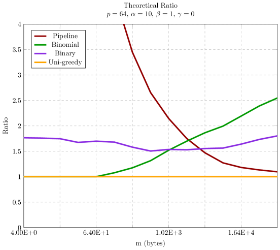
(a) Message size versus ratio

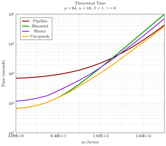
(b) Message size versus time

Figure 4: Theoretical results for $p=64$ plotting message size ($m$) versus ratio (4a) and time (4b) in a unidirectional system. The machine parameters are fixed at $\alpha=10$, $\beta=1$, and $\gamma=0$.

Figures 4a, 4b, and 5 show the results for when $\alpha=10$, $\beta=1$, and $\gamma=0$. In Figure 4a and 4b, the number of processors is fixed at 64. In Figure 4a the algorithms are compared by plotting the ratio between the algorithms time and the time for the uni-greedy algorithm. For small messages the optimal segment size for uni-greedy is 1, and uni-greedy is exactly the binomial algorithm. So for small messages, ($m<64$ bytes in this example) uni-greedy and binomial have the same time. For large messages ($m>1.64\times 10^{4}$ bytes in this example), the poor start up of the pipeline algorithm is negligible and the pipeline algorithm approaches the uni-greedy algorithm asymptotically. The middle region is where uni-greedy is the most relevant, seeing an increase in performance over the standard algorithms up to approximately 50% faster. Figure 4b plots the time for each algorithm.

Figure 5 gives the results for each value of $p$ and $m$, the uni-greedy algorithm is compared with the best of the standard algorithms by plotting

$$\textmd{Ratio}=\dfrac{\textmd{Minimum time of the standard algorithms}}{\textmd{Time for the Greedy Algorithm}}.$$

A ratio of 1 (white in the figure) indicates that a standard algorithm has the same time as the uni-greedy algorithm. Larger numbers indicate a more significant improvement. Again the region that uni-greedy provides the greatest improvement is for “medium” size messages. As the number of processors increase, the range of message sizes where uni-greedy provides the most improvement (ratio $\approx$ 1.5) increases. This is largely due to the difference in the number of time steps required to reduce the first segment of uni-greedy ($\lceil log_{2}p\rceil$) versus that of pipeline ($p-1$). For larger $p$, pipeline requires a larger message before it is able to “make up” for the extra time to reduce the first segment.

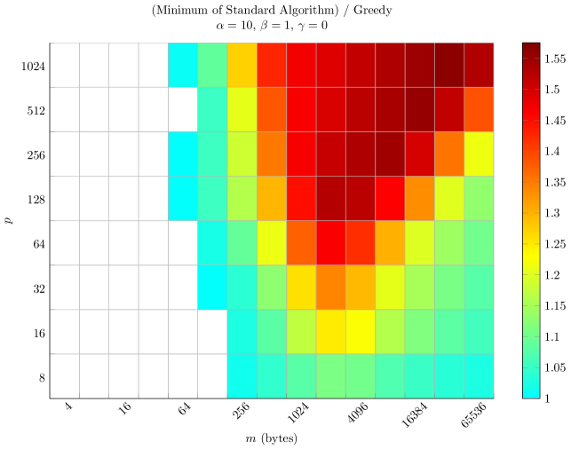
Figure 5: Ratio between the time for the best standard algorithm and the uni-greedy algorithm for varying values of $p$ (number of processors) and $m$ (message size). The machine parameters are fixed at $\alpha=10$, $\beta=1$, and $\gamma=0$.

VI Bidirectional System

Binomial	Time	$\lceil log_{2}p\rceil(\alpha+\beta m+\gamma m)$
Pipeline	Time	$(p+q-2)(\alpha+\beta s+\gamma s)$
	$s_{opt}$	$\left(\dfrac{m\alpha}{(p-2)(\beta+\gamma)}\right)^{1/2}$
	$T_{opt}$	$\left[\left((p-2)\alpha\right)^{1/2}+\left(m(\beta+\gamma)\right)^{1/2}\right]^{2}$
Binary	Time	$2\left(\lceil log_{2}(p+1)\rceil+q-1\right)(\alpha+\beta s+\gamma s)$
	$s_{opt}$	$\left(\dfrac{m\alpha}{(N-2)(\beta+\gamma)}\right)^{1/2}$
	$T_{opt}$	$2\left[\left((N-2)\alpha\right)^{1/2}+\left(m(\beta+\gamma)\right)^{1/2}\right]^{2}$
Bi-greedy & Optimal Broadcast	Time	$(\lceil\log_{2}p\rceil+q-1)(\alpha+\beta s+\gamma s)$
	$s_{opt}$	$\left(\dfrac{m\alpha}{(\lceil\log_{2}p\rceil-1)(\beta+\gamma)}\right)^{1/2}$
	$T_{opt}$	$\left[\left((\lceil\log_{2}p\rceil-1)\alpha\right)^{1/2}+\left(m(\beta+\gamma)\right)^{1/2}\right]^{2}$
Butterfly	Time	$2\lceil\log_{2}p\rceil\alpha+2\frac{p-1}{p}\beta m+\frac{p-1}{p}\gamma m$

TABLE III: Time analysis for bidirectional reduction algorithms, where $N=\lceil\log_{2}(p+1)\rceil$, $s_{opt}$ is the optimal equi-segment size, and $T_{opt}$ is the time for the algorithm at $s_{opt}$. Formulae are valid for $p>3$. The reduce-scatter/gather formula is only a lower bound when $p$ is not a power of two.

In this section, we can adapt the uni-greedy algorithm presented in Section V under the unidirectional context to an algorithm more suited for a bidirectional system. We wish to compare the new algorithm to the current state-of-the-art. We again have the standard algorithms: binomial, binary, and pipeline. We also consider a butterfly algorithm [4, 5] which minimizes the computation term of the reduction. All of the algorithms mentioned so far work for non-commutative operations. If the operation is commutative, then any broadcast algorithm can be used (in reverse) for a reduction. Bar-Noy, et al. [2] and Träff and Ripke [3] provide broadcast algorithms that match the lower bound on the number of communication rounds for broadcasting $q$ segments among $p$ processors. The time complexity for such a reduction algorithm is

$$(\lceil\log_{2}p\rceil+q-1)(\alpha+\beta m+\gamma m).$$

From theoretical simulations it is seen that our new algorithm (bi-greedy) has the same time complexity of a reverse optimal broadcast. The rest of this section is organized as follows: In Section VI-A we analyze the time complexity of the reduction algorithms. In Section VI-B we introduce the new algorithm (bi-greedy).

VI-A Theoretical Results

We begin by summarizing the time complexity for each algorithm in Table III. Binomial and butterfly do not have a choice on the segment size, so the optimal segment/time rows are not included for those algorithms. Binomial, binary, pipeline, and bi-greedy, all work in the same way: the message is split into $q$ segments of equi-segment size and segments are communicated in rounds, where the time for one round is $\alpha+\beta s+\gamma s$. For these algorithms it is clear that bi-greedy is the best since it require the minimum number of rounds for any number of segments. The butterfly algorithm does not start with a fixed segmentation of the message, but rather recursively halves the message size and exchanges the message between processors. This method allows the computation to be distributed evenly among the processors and hence minimizing the computational term II. If the computational rate is small (i.e. $\gamma$ is large) than minimizing the computation term can be advantageous.

Figure 6a and 6b show the results for when $p=64$, $\alpha=50000$, $\beta=6$ and $\gamma=1$. In Figure 6a the ratio between the time of the algorithm and the time of bi-greedy is shown. When comparing bi-greedy with binomial, binary, and pipeline, we see similar results as in the unidirectional case. For small messages ($m<10$ KB in this example), bi-greedy and binomial have the same time. For large messages ($m>10^{5}$ KB in this example), pipeline approaches the bi-greedy algorithm asymptotically. For medium length messages ($200<m<4000$ KB in this example), bi-greedy provides approximately a 50% increase in performance. In this example, the butterfly algorithm performs well for medium size messages ($m\approx 300$ KB in this example) but does not provide good asymptotic behavior for large and small message sizes. This is not a surprise as Rabenseifner provides tuning experiments to switch to the binomial algorithm for small messages, and the pipeline algorithm for large messages [4].

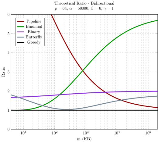
(a) Message size versus ratio

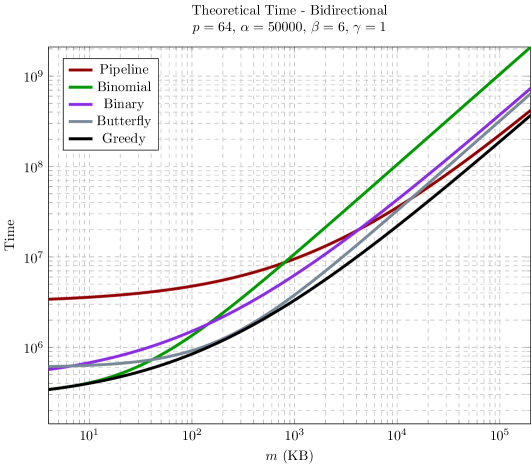
(b) Message size versus time

Figure 6: Theoretical results for bidirectional system when $p=64$ plotting message size ($m$) versus ratio (6a) and time (6b). The formula for the reference line is $\lceil\log_{2}p\rceil\alpha+m\beta+\frac{p-1}{p}m\gamma,$ which is the sum of the lower bounds for each term: $\alpha$, $\beta$, $\gamma$. The machine parameters are fixed at $\alpha=50000$, $\beta=6$, and $\gamma=1$.

For some machine parameters the butterfly algorithm can perform better than bi-greedy for some message sizes. If the ratio, $\beta/\gamma$, is small enough then for some message sizes the butterfly algorithm will be better than bi-greedy. To be more precise as to what constitutes a small ratio we consider Figure 7. Above the blue line bi-greedy will always be better than the butterfly algorithm. Below the blue line, there exists a message size, $m$, such that the butterfly algorithm is better than bi-greedy (in Figure 6 butterfly would dip below bi-greedy). For up to 1000 processors the ratio would have to be less than 5 for the butterfly algorithm to be better. In practice, a ratio larger than 10 is more likely, even for single core processors.

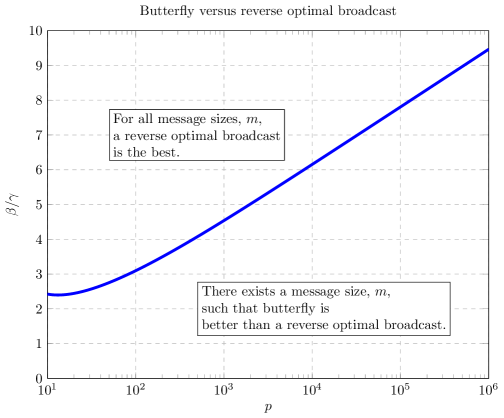
Figure 7: Parameters for which there exists a message size, $m$, such that the butterfly algorithm is better than a reverse optimal broadcast algorithm.

VI-B The Bi-greedy Algorithm

In the unidirectional case, the optimal algorithm attempted to fill all available ports at any time. This is the goal when adapting to the bidirectional case. The difference is that a processor has two ports (one sending and one receiving) rather than a single port that either sends or receives.

The bidirectional greedy (bi-greedy) algorithm adheres to the following restrictions: the message is split using equi-segmentation and the ports are filled giving priority to segments with smaller indices. This restriction differs from that of uni-greedy, in that a processor may receive a segment before sending a segment with a smaller index. For the uni-greedy algorithm, the smaller indexed segment must be sent first. A downfall of this relaxation is that extra storage must be allocated. However, other reduction algorithms also require a larger buffer (see Rabenseifner [4]).

$S=\textmd{zeros}(p,1)$;

$R=\textmd{zeros}(p,1)$;

$C=\textmd{zeros}(p,2)$;

$t=0$;

$M=\textmd{zeros}(p,q)$;

while  $\min\{M(i,j)\;|\;1\leq i\leq p\;\textmd{and}\;1\leq j\leq q\}=0$ do

      

      $\textmd{segStart}=\min\{j\;|\;M(1,j)=0\}$;

       $\textmd{stop}=1$;

       $j=\textmd{segStart}-1$;

      

      while  stop  do

             $j\leftarrow j+1$;

             $\textmd{COMP}=\{i\;|\;C(i,1)\leq t<C(i,2)\;\textmd{or}\;t+t_{comm}(j)>C(i)\}$;

             $I=\{i\;|\;M(i,j)=0\}$;

             $\textmd{sendProc}=I\setminus\textmd{COMP}\setminus\{i\;|\;S(i)>t\}$;

             $\textmd{recvProc}=I\setminus\textmd{COMP}\setminus\{i\;|\;R(i)>t\}$;

            

            $\textmd{freeProc}=\textmd{sendProc}\bigcap\textmd{recvProc}$;

             $\textmd{sendProc}\leftarrow\textmd{sendProc}\setminus\textmd{freeProc}$;

             $\textmd{recvProc}\leftarrow\textmd{recvProc}\setminus\textmd{freeProc}$;

            

            $s=|\textmd{sendProc}|$;

             $r=|\textmd{recvProc}|$;

             $f=|\textmd{freeProc}|$;

            

            if  $s=r$  then

                   $y=\lfloor f/2\rfloor$;

                   $\textmd{sendProc}\leftarrow\textmd{sendProc}\bigcup\{\textmd{freeProc}(i)\;|\;f-y+1\leq i\leq f\}$;

                   $\textmd{recvProc}\leftarrow\textmd{recvProc}\bigcup\{\textmd{freeProc}(i)\;|\;1\leq i\leq y\}$;

                  

             else if  $s<r$ then

                   $y=r-s$;

                   $m=\min(f,y)$;

                   $x=\lfloor(f-m)/2\rfloor$;

                   if  $m>0$ then

                         $\textmd{sendProc}\leftarrow\textmd{sendProc}\bigcup\{\textmd{freeProc}(i)\;|\;(f-(m+x)+1\leq i\leq f\}$;

                  if  $x>0$ then

                         $\textmd{recvProc}\leftarrow\textmd{recvProc}\bigcup\{\textmd{freeProc}(i)\;|\;1\leq i\leq x\}$;

                  

             else if  $r<s$ then

                   $y=s-r$;

                   $m=\min(f,y)$;

                   $x=\lfloor(f-m)/2\rfloor$;

                   if  $m>0$ then

                         $\textmd{recvProc}\leftarrow\textmd{recvProc}\bigcup\{\textmd{freeProc}(i)\;|\;1\leq i\leq m+x\}$;

                  if  $x>0$ then

                         $\textmd{sendProc}\leftarrow\textmd{sendProc}\bigcup\{\textmd{freeProc}(i)\;|\;f-x+1\leq i\leq f\}$;

                  

            

            $l=\min(|\textmd{sendProc}|,|\textmd{recvProc})$

             if  $l=0$  then

                   $\textmd{sendProc}\leftarrow\emptyset$;

                   $\textmd{recvProc}\leftarrow\emptyset$;

                  

             else

                   $\textmd{sendProc}=\{\textmd{sendProc}(i)\;|\;1\leq i\leq l\}$;

                   $\textmd{recvProc}=\{\textmd{recvProc}(i)\;|\;1\leq i\leq l\}$;

                  

            $M(i,j)=t+t_{comm}(j),\forall\;i\;\textmd{s.t.}\;i\in\textmd{sendProc}$;

             $S(i)=t+t_{comm}(j),\forall\;i\;\textmd{s.t.}\;i\;\in\textmd{sendProc}$;

             $R(i)=t+t_{comm}(j)+t_{comp}(j),\forall\;i\;\textmd{s.t.}\;i\in\textmd{recvProc}$;

             $C(i,1)=t+t_{comm}(j),\forall\;i\;\textmd{s.t.}\;i\in\textmd{recvProc}$;

             $C(i,2)=t+t_{comm}(j)+t_{comp}(j),\forall\;i\;\textmd{s.t.}\;i\in\textmd{recvProc}$;

            

            if  $|\{i\;|\;M(i,j)=0\}|=1$  then

                   $M(1,j)=max(\{M(i,j)\;|\;1\leq i\leq p\})+t_{comp}(j)$;

            

            if  $|\{i\;|\;S(i)\leq t\}|+|\{i\;|\;R(i)\leq t\}|<2$ then

                   $\textmd{stop}=0$;

             else if $j\geq q$ then

                   $\textmd{stop}=0$;

            

      $t=t+1$;

      

Algorithm 2 Bi-greedy Algorithm

Algorithm 2 on the next page gives the pseudo-code for the bi-greedy algorithm. $S$ and $R$ are $p\times 1$ arrays where entry $i$ gives the time when processor $i-1$ has finished sending or receiving, respectively, the last scheduled communication. $C$ is a $p\times 2$ array where $C(i,1)$ is the start time and $C(i,2)$ is the end time of the last scheduled computation on processor $i-1$. $M$ is a $p\times q$ array where entry $(i,j)$ gives the time when processor $i-1$ has finished sending segment $j$ (except for the root ($i=1$) which gives the time after finishing the final computation). In each inner loop the maximum number of send/receive pairs for segment $j$ is determined. The final entries of sendProc and recvProc are scheduled to send and receive segment $j$, respectively. These processors are paired entry-wise to obtain send/receive pairs. The algorithm assumes a discrete time step.

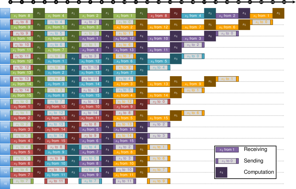
Figure 8: Bi-greedy algorithm for 16 processors and 5 equi-segments for $t_{comm}=2$ and $t_{comp}=1$. Each color represents a different segment. Solid rectangles represent receiving processors and rectangles with end strips represent sending processors. The darker rectangles represent computation.

Figure 8 gives an example for 16 processors and 5 equi-segments with $t_{comm}=2$ and $t_{comp}=1$. For this example we see that the time complexity matches the that of the optimal broadcast algorithm. From experiments we conjecture that for all $p$ and $q$ the bi-greedy algorithm has the same time complexity as a reverse optimal broadcast algorithm. We do not provide a proof at this time.

VII Numerical Results

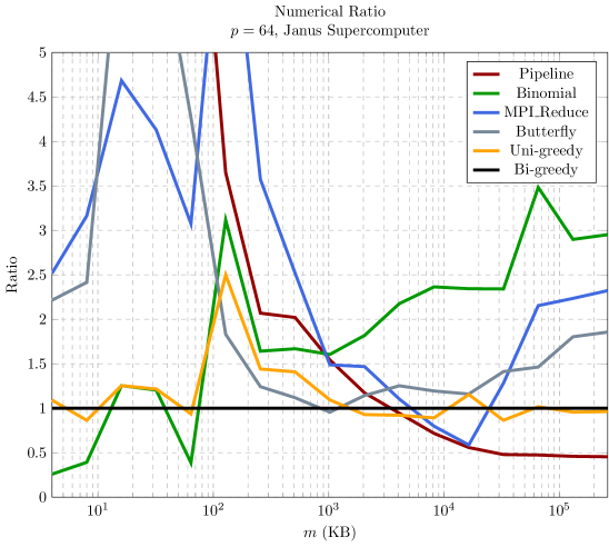
(a) Message size versus ratio

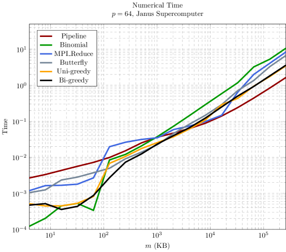
(b) Message size versus time

Figure 9: Experimental results for each algorithm for all possible message sizes for 64 processors.

For the numerical experiments we implemented the uni-greedy algorithm developed under the unidirectional contexted (Figure 2) and the bi-greedy algorithm developed under the bidirectional context (Algorithm 2). The algorithms were implemented using OpenMPI version 1.4.3. All experiments were performed on the Janus supercomputer which consists of 1,368 nodes with each node having 12 cores. Since processors on a single node have access to shared memory, only one processor per node was used with a total of 64 nodes in use for the experiments. The nodes are connected using a fully non-blocking quad-data-rate (QDR) InfiniBand interconnect. The time for a reduction was calculated by taking the minimum time of 10 experiments.

We wish to compare the algorithms assuming that each is optimally tuned for the best segmentation. For a message of size $m$, segments of size $2^{i},\;\textmd{s.t.}\;i=0,\dots,\lfloor\log_{2}m\rfloor$, where tested and the best time was taken to be the time of an optimally tuned algorithm. Figures 9a and 9b compares the optimally tuned greedy algorithms with other algorithms for reduction.

Comparing bi-greedy with binomial and pipeline shows similar results as to those of the theoretical results. For small messages, the time for binomial and greedy are close, although binomial performs about twice as well as greedy in a few cases. For large messages, pipeline begins to out perform all algorithms and is a factor of two better than bi-greedy. However, for medium size messages ($100<m<3000$ KB) bi-greedy is better than both binomial and pipeline. The binary algorithm was not analyzed experimentally.

Comparing bi-greedy with the butterfly algorithm again shows similar results to the theoretical case. The bi-greedy algorithm outperforms butterfly for almost all message sizes. The butterfly algorithm performs very well for medium size messages (about the same time as bi-greedy for $m=1000$ KB), but has poor performance for large and small messages. Comparing the bi-greedy algorithm with the built-in MPI function MPI_Reduce, shows that greedy, in most cases, is the best. Finally, the uni-greedy algorithm (although designed for a unidirectional system) performed fairly well in general, matching the performance of bi-greedy for small and large messages.

For small messages, greedy is equivalent to binomial, but there is a fairly large difference in the performance in this region. This is because the two algorithms implemented use different send/receive pairings and the performance differences indicate the system is actually heterogeneous.

Checking all of the possible segment sizes for a given message size is not practical. Auto-tuning could be used to determine the optimal segmentation for different message sizes.

VIII Unequal segmentation

So far we have only optimized the greedy algorithm by splitting a message into equally sized segments (except possibly the last segment). An immediate question is then asked, what if the segments have unequal size? A question we have not found to be considered in the literature. Can the existing algorithms be improved?

To investigate these questions the message size was fixed to $m=10$ and all possible segmentations were checked for $\alpha=0,1,\dots,10,20,30,\dots,100,200,300,\dots,1000$, $\beta=1$, $\gamma=0,1$, and $p=2^{n}\;\mbox{s.t.}\;n=2,\dots,10$ and $p=3(2^{n})\;\mbox{s.t.}\;n=1,\dots,9$. There a total of 512 possible segmentations. Examples of possible segmentations are $(9,1)$, $(3,3,3,1)$, $(3,2,4,1)$, $(2,2,1,5)$, $(6,3,1)$, etc. An equi-segmentation is said to be one that has the same segment size for all segments except possibly the last segment may be smaller.

For the greedy algorithm, 61 out of 986 experiments where optimized by an unequal segmentation. To compare unequal to equi-segmentation, we use the value

$$\textmd{ Ratio }=\dfrac{\textmd{ Best time for equi-segmentations}}{\textmd{Best time for all segmentations}}.$$

A ratio of 1 indicates that one of the optimal segmentations is an equi-segmentation. If there were multiple segmentations that were optimal and one of them was an equal segmentation, then the experiment was said to be optimized by an equi-segmentation. The maximum improvement over equi-segmentation was 7.3%. Of the 61 that did see and increase in performance the average improvement was 2.0%.

Parameters Ratio Equi-segmentation Optimal Segmentation $p=6,\alpha=1,\gamma=1$ 1.0408 (4,4,2) (5,3,2) (3,5,2) (3,4,2,1) (4,2,2,2) (2,4,2,2) (3,2,2,2,1) (2,3,2,2,1) $p=6,\alpha=2,\gamma=1$ 1.0357 (4,4,2) (5,3,2) (3,5,2) $p=8,\alpha=0,\gamma=1$ 1.0571 (1,1,1,1,1,1,1,1,1,1) (2,1,1,1,1,1,1,1,1) $p=8,\alpha=1,\gamma=1$ 1.0200 (4,4,2) (5,2,2,1) (3,4,2,1) $p=12,\alpha=0,\gamma=1$ 1.0732 (1,1,1,1,1,1,1,1,1,1) (2,2,1,1,1,1,1,1) $p=12,\alpha=1,\gamma=1$ 1.0169 (4,4,2) (3,3,1,2,1) (2,2,1,2,2,1) $p=12,\alpha=3,\gamma=1$ 1.0130 (5,5) (4,5,1) $p=16,\alpha=1,\gamma=0$ 1.0526 (3,3,3,1) (5,3,2) (4,2,2,2) $p=16,\alpha=1,\gamma=1$ 1.0161 (3,3,3,1) (3,2,2,2,1) $p=16,\alpha=2,\gamma=1$ 1.0278 (4,4,2) (4,3,3) $p=24,\alpha=3,\gamma=1$ 1.0108 (3,3,3,1) (5,4,1) (4,3,3) $p=24,\alpha=4,\gamma=1$ 1.0388 (5,5) (5,4,1) (4,3,3) $p=32,\alpha=1,\gamma=0$ 1.0222 (4,4,2) (3,3,2,2) $p=32,\alpha=1,\gamma=1$ 1.0141 (2,2,2,2,2) (3,2,2,2,1) $p=32,\alpha=2,\gamma=1$ 1.0118 (4,4,2) (4,3,3) (5,2,2,1) (3,3,2,2) $p=32,\alpha=3,\gamma=1$ 1.0104 (4,4,2) (4,3,3) $p=48,\alpha=1,\gamma=0$ 1.0408 (4,4,2) (4,2,2,2) (3,2,3,2) $p=48,\alpha=1,\gamma=1$ 1.0260 (2,2,2,2,2) (3,2,2,2,1) (2,2,1,2,2,1) $p=48,\alpha=2,\gamma=0$ 1.0164 (4,4,2) (5,3,2) $p=48,\alpha=2,\gamma=1$ 1.0215 (3,3,3,1) (3,3,2,2) $p=48,\alpha=3,\gamma=1$ 1.0093 (4,4,2) (4,3,3) (3,4,3) (3,3,2,2) (3,2,3,2) $p=48,\alpha=4,\gamma=1$ 1.0084 (4,4,2) (5,4,1) (5,2,3) (4,3,3) (3,4,3) $p=64,\alpha=1,\gamma=1$ 1.0253 (3,3,3,1) (3,2,2,2,1) (2,2,2,2,1,1) (2,2,2,1,2,1) (2,2,2,1,1,1,1) (2,2,1,1,1,1,1,1) $p=64,\alpha=2,\gamma=1$ 1.0106 (3,3,3,1) (3,3,2,2) $p=64,\alpha=3,\gamma=1$ 1.0093 (4,4,2) (3,3,2,2) $p=96,\alpha=1,\gamma=0$ 1.0182 (4,4,2) (3,3,2,2) (3,2,3,2) (2,3,3,2) $p=96,\alpha=1,\gamma=1$ 1.0119 (1,1,1,1,1,1,1,1,1,1) (2,2,2,2,1,1) (2,2,2,1,1,1,1) (2,2,1,1,1,1,1,1) $p=96,\alpha=2,\gamma=1$ 1.0098 (3,3,3,1) (3,3,2,2) $p=96,\alpha=3,\gamma=1$ 1.0085 (3,3,3,1) (3,3,2,2) $p=128,\alpha=1,\gamma=1$ 1.0116 (2,2,2,2,2) (2,2,2,1,1,1,1) (2,1,1,1,1,1,1,1,1) (1,1,1,2,1,1,1,1,1) $p=192,\alpha=1,\gamma=0$ 1.0169 (3,3,3,1) (2,2,2,2,1,1)

Parameters Ratio Equi-segmentation Optimal Segmentation $p=256,\alpha=1,\gamma=0$ 1.0161 (2,2,2,2,2) (4,3,2,1) (3,2,3,2) (2,3,3,2) (3,3,2,1,1) (2,2,3,2,1) (2,3,2,1,1,1) (3,2,1,2,1,1) (3,1,2,2,1,1) (2,2,2,2,1,1) (3,2,1,1,2,1) (3,1,2,1,2,1) (2,2,2,1,2,1) (2,2,1,2,2,1) (2,1,2,2,2,1) (1,2,2,2,2,1) (2,1,2,2,1,2) $p=256,\alpha=1,\gamma=1$ 1.0109 (1,1,1,1,1,1,1,1,1,1) (2,1,2,1,1,1,1,1) (2,1,1,1,1,1,1,1,1) $p=256,\alpha=2,\gamma=0$ 1.0256 (4,4,2) (5,3,2) (4,3,3) $p=256,\alpha=2,\gamma=1$ 1.0085 (2,2,2,2,2) (3,2,3,2) (2,2,2,3,1) (2,1,2,2,2,1) (2,1,2,2,1,1,1) $p=256,\alpha=3,\gamma=0$ 1.0217 (4,4,2) (4,3,3) $p=256,\alpha=3,\gamma=1$ 1.0224 (3,3,3,1) (3,2,3,2) $p=256,\alpha=4,\gamma=1$ 1.0265 (3,3,3,1) (5,3,2) (4,3,3) $p=256,\alpha=5,\gamma=1$ 1.0303 (4,4,2) (5,3,2) $p=256,\alpha=6,\gamma=1$ 1.0279 (4,4,2) (5,3,2) $p=384,\alpha=3,\gamma=1$ 1.0142 (3,3,3,1) (3,2,3,2) (2,3,3,2) $p=512,\alpha=1,\gamma=0$ 1.0154 (2,2,2,2,2) (2,2,2,2,1,1) (2,2,2,1,2,1) $p=512,\alpha=2,\gamma=0$ 1.0238 (4,4,2) (4,3,3) $p=512,\alpha=3,\gamma=0$ 1.0100 (4,4,2) (4,3,3) $p=512,\alpha=3,\gamma=1$ 1.0069 (3,3,3,1) (3,2,3,2) (2,3,3,2) $p=512,\alpha=4,\gamma=1$ 1.0061 (3,3,3,1) (2,3,3,2) $p=512,\alpha=5,\gamma=1$ 1.0167 (4,4,2) (4,3,3) $p=512,\alpha=6,\gamma=1$ 1.0154 (4,4,2) (4,3,3) $p=512,\alpha=7,\gamma=1$ 1.0095 (4,4,2) (4,3,3) $p=768,\alpha=1,\gamma=0$ 1.0147 (2,2,2,2,2) (2,2,2,2,1,1) (2,2,2,1,2,1) (2,1,2,2,2,1) (1,2,2,2,2,1) $p=768,\alpha=1,\gamma=1$ 1.0099 (1,1,1,1,1,1,1,1,1,1) (2,1,1,1,1,1,1,1,1) $p=768,\alpha=2,\gamma=0$ 1.0111 (3,3,3,1) (4,3,3) (3,4,2,1) (4,2,3,1) (3,2,3,2) (2,3,3,2) (2,2,4,2) (2,2,3,3) $p=768,\alpha=3,\gamma=0$ 1.0189 (4,4,2) (4,3,3) $p=768,\alpha=3,\gamma=1$ 1.0066 (2,2,2,2,2) (2,3,3,2) $p=768,\alpha=4,\gamma=0$ 1.0164 (4,4,2) (4,3,3) $p=768,\alpha=4,\gamma=1$ 1.0174 (3,3,3,1) (3,2,3,2) (2,3,3,2) $p=768,\alpha=5,\gamma=1$ 1.0317 (3,3,3,1) (4,3,3) $p=768,\alpha=6,\gamma=1$ 1.0341 (4,4,2) (4,3,3) $p=768,\alpha=7,\gamma=1$ 1.0270 (4,4,2) (4,3,3) $p=768,\alpha=8,\gamma=1$ 1.0209 (4,4,2) (4,3,3) $p=1024,\alpha=3,\gamma=0$ 1.0093 (4,4,2) (4,3,3)

TABLE IV: Optimal Segmentation compared to best of the equi-segmentations.

Table IV shows results for all experiments that were optimized by unequal segmentation. We note that, in all cases, one of the optimal segmentations was nearly the same as the best equi-segmentation. Actually, to obtain the optimal (unequal) segmentation from the best of the equi-segmentations, the size of only one or two segments had to be increased or decreased by a value of 1 in most cases.

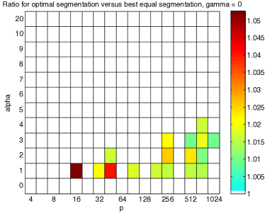
(a) $\gamma=0$

(b) $\gamma=1$

Figure 10: Ratio for optimal segmentation versus the best equal segmentation.

Figures 10a and 10b show the results for all $\alpha$, $\gamma$, and $p$. For $\alpha>20$, the greedy algorithm was always optimized by an equi-segmentation and therefore is not graphed. A pattern as to when unequal segmentation is optimal is not evident from the figures. For the pipeline algorithm, all experiments where optimized by equi-segmentation. The binary algorithm was not checked for unequal segmentation.

The experiment is limited to small values of $m$ since the number of possible segmentations grows exponentially as $m$ increases. The algorithms were not implemented for unequal segmentations since the small theoretical improvements most likely will not be obtained. Further investigation is required to determine if for larger messages sizes does the improvement of unequal segmentation become greater.

IX Conclusion

Two new algorithms for reduction are presented. The two algorithms are developed under two different communication models (unidirectional and bidirectional).

We prove that the unidirectional algorithm is optimal under certain assumptions. Our assumptions are fully connected, homogeneous system, and processing the segments in order. Previous algorithms that satisfy the same assumptions are only appropriate for some configurations. The uni-greedy algorithm is optimal for all configurations. The most improvement over standard algorithms is for messages of “medium” length, providing about 50% improvement when compared to the best of the standard algorithms in that region. The region of “medium” length messages become more prevalent as the number of processors increases.

We adapted the greedy algorithm that was developed in the unidirectional context to an algorithm that was more suited for a bidirectional system. With simulations we found that the bi-greedy algorithm matched the time complexity of optimal broadcast algorithms (scheduled in reverse order as a reduction). Similar performance improvements where found as in the unidirectional case.

Implementation of the algorithms confirm the theoretical results. Our implementation of the bi-greedy algorithm is was best among all algorithms implemented for “medium” size messages. For small and large messages, the more simplistic algorithms (binomial and pipeline), which are asymptotically optimal, outperformed the greedy algorithms.

Finally, the concept of unequal segmentation was discussed and analyzed for the greedy algorithm and the pipeline algorithm in a unidirectional system. For the greedy algorithm, unequal segmentation provided, in our sample test suite, the optimal segmentation $6.2\%$ of the time with a maximum improvement of 7.3%. The pipeline algorithm was always optimized by equal segmentation.

References

- [1] R. Hockney, “The communication challenge for MPP: Intel Paragon and Meiko CS-2.” Parallel Computing, vol. 20, no. 3, pp. 389–398, 1994.
- [2] A. Bar-Noy, S. Kipnis, and B. Schieber, “Optimal multiple message broadcasting in telephone-like communication systems,” Discrete Appl. Math., vol. 100, no. 1-2, pp. 1–15, Mar. 2000. [Online]. Available: http://dx.doi.org/10.1016/S0166-218X(99)00155-9
- [3] J. L. Träff and A. Ripke, “Optimal broadcast for fully connected processor-node networks,” J. Parallel Distrib. Comput., vol. 68, no. 7, pp. 887–901, 2008.
- [4] R. Rabenseifner, “Optimization of collective reduction operations,” in International Conference on Computational Science, 2004, pp. 1–9.
- [5] R. Rabenseifner and J. L. Träff, “More efficient reduction algorithms for non-power-of-two number of processors in message-passing parallel systems,” in PVM/MPI, 2004, pp. 36–46.
- [6] P. Sanders, J. Speck, and J. L. Träff, “Two-tree algorithms for full bandwidth broadcast, reduction and scan,” Parallel Computing, vol. 35, no. 12, pp. 581 – 594, 2009, selected papers from the 14th European PVM/MPI Users Group Meeting. [Online]. Available: http://www.sciencedirect.com/science/article/pii/S0167819109000957
- [7] O. Beaumont, A. Legrand, L. Marchal, and Y. Robert, “Pipelining broadcasts on heterogeneous platforms,” Parallel and Distributed Systems, IEEE Transactions on, vol. 16, no. 4, pp. 300 – 313, April 2005.
- [8] O. Beaumont, L. Marchal, and Y. Robert, “Broadcast trees for heterogeneous platforms,” in 19th International Parallel and Distributed Processing Symposium IPDPS’2005. Society Press, 2005, pp. 3–8.
- [9] A. Legrand, L. Marchal, and Y. Robert, “Optimizing the steady-state throughput of scatter and reduce operations on heterogeneous platforms,” J. Parallel Distrib. Comput., vol. 65, no. 12, pp. 1497–1514, Dec. 2005. [Online]. Available: http://dx.doi.org/10.1016/j.jpdc.2005.05.021
- [10] E. Chan, R. A. van de Geijn, W. Gropp, and R. Thakur, “Collective communication on architectures that support simultaneous communication over multiple links,” in PPOPP, 2006, pp. 2–11.
- [11] S. S. Vadhiyar, G. E. Fagg, and J. Dongarra, “Automatically tuned collective communications,” in Proceedings of the 2000 ACM/IEEE conference on Supercomputing (CDROM), ser. Supercomputing ’00. Washington, DC, USA: IEEE Computer Society, 2000. [Online]. Available: http://dl.acm.org/citation.cfm?id=370049.370055
- [12] J. Pjesivac-Grbović, T. Angskun, G. Bosilca, G. Fagg, E. Gabriel, and J. Dongarra, “Performance analysis of MPI collective operations,” in Parallel and Distributed Processing Symposium, 2005. Proceedings. 19th IEEE International, april 2005, p. 8 pp.
- [13] E. Chan, M. Heimlich, A. Purkayastha, and R. van de Geijn, “On optimizing collective communication,” in CLUSTER ’04 Proceedings of the 2004 IEEE International Conference on Cluster Computing, 2004, pp. 145–156.
- [14] M. Cosnard and Y. Robert, “Complexity of parallel QR factorization,” Journal of the A.C.M., vol. 33, no. 4, pp. 712–723, 1986.