LOW ENERGY $\alpha-\alpha$ SEMIMICROSCOPIC POTENTIALS

Abstract

The $\alpha-\alpha$ interaction potential is obtained within the double folding model with density-dependent Gogny effective interactions as input. The one nucleon knock-on exchange kernel including recoil effects is localized using the Perey-Saxon prescription at zero energy. The Pauli forbidden states are removed thanks to successive supersymmetric transformations. Low energy experimental phase shifts, calculated from the variable phase approach, as well as the energy and width of the first $0^{+}$ resonance in ⁸Be are reproduced with high accuracy.

(Received )

Key words: Gogny interaction, knock-on nonlocal kernel, variable phase equation, SUSY potential.

1 INTRODUCTION

In last time there is an increasing interest in understanding the properties of $\alpha$-matter mainly due to the believe that this type of hadronic matter occurs in astrophysical environment in unconfined form. In the debris of a supernova explosion, a substantial fraction of hot and dense matter resides in $\alpha$-particles and therefore the equation of state of subnuclear matter is essential in simulating the supernova collapse and explosions and is also important for the formation of the supernova neutrino signal [1].

The basic ingredient in the calculation of the ground state alpha matter [2] as well in the $\alpha$-cluster model of nuclei [3] is the $\alpha-\alpha$ interaction potential. This has been studied extensively using both local and nonlocal interactions. Among the most important are those using the resonating group model (RGM) [4, 5], the energy and angular momentum independent potential model of Buck, Friedrich and Wheatley [6] and the phenomenological potential of Ali and Bodmer [7]. There have been proposed several versions of the Ali-Bodmer potential: a Gaussian potential with a stronger repulsive component by Langanke and Müller [8], as well a version with a softer repulsive component by Yamada and Schuck [9]. All these models predict potentials quite different in strength and range but all are claimed to reproduce experimental data up the the breakup threshold.

Microscopic RGM calculations by Schmid and Wildermuth [5] lead to the important conclusion that due to the compact structure and the large binding energy the radius of the $\alpha$-particle stays essentially the same during the compound system formation and therefore the polarization effects could be neglected. This observation substantiates the idea of calculation of a $\alpha-\alpha$ potential from the double folding model.

We propose in this paper to generate the $\alpha-\alpha$ potential within the double folding model using the Gogny force as input. Previously Sofianos et al.[10] derived the $\alpha-\alpha$ potential using the energy density formalism based on Skyrme effective interaction.

However, the potential issued from double-folding calculation, even corrected by knock-on exchange terms, is generally too deep due to the presence of forbidden bound states. These states have a clear interpretation within the RGM model: they are redundant solutions giving fully antisymmetrized wave functions that vanish identically. These latter bound states are eliminated thanks to successive supersymmetric transformations as given in [11], which preserves the continuous spectrum (phase-shift) and resonances [12].

In section 2 we present the derivation of the $\alpha-\alpha$ interaction. In section 3 the derivation and the properties of supersymmetric partner are presented. Our conclusions are given in section 4.

2 Bare $\alpha-\alpha$ interaction : double-folding with Gogny forces

Since the potentials providing saturation at lower densities of the alpha matter are highly schematic (infinite repulsive short-range interactions) we turn to a calculation of the bare $\alpha-\alpha$ interaction based on the double-folding method for two ions at energies around the barrier, starting with realistic densities of the $\alpha$-particle and modern effective nucleon-nucleon interactions.

Within the double-folding model [13] the interaction between two alpha clusters is calculated as a convolution of a local two-body potential $v_{nn}$ and the single particle densities of the two clusters, namely

$$v_{\alpha\alpha}(\vec{r})=\int d\vec{r}_{1}\int d\vec{r}_{2}\rho_{\alpha}({r}_{1})\rho_{\alpha}({r}_{2})v_{nn}(\rho,\vec{r}-\vec{r}_{1}+\vec{r}_{2})$$ (1)

The effective $n-n$ interaction $v_{nn}$ is taken to be density-dependent as expected from a realistic interaction. It depends on the density $\rho$ of the nuclear matter where the two interacting nucleons are embedded. For the sake of simplicity, we choose Gaussians interactions in order to have the most tractable analytical calculations. A candidate satisfying this requirement is provided by the Gogny forces [14]. In this paper, we will report results using three main parametrizations of the Gogny interaction [14], denoted D1 and D1S [15] as well as the most recent variant, labeled D1N [16].

We remind that the standard form of the Gogny interactions is,

$$v_{nn}(r) =\sum_{i=1}^{2}(W+BP_{\sigma}-HP_{\tau}-MP_{\sigma}P_{\tau})e^{-r^{2}/\mu_{i}^{2}}$$ (2)

$$+t_{3}(1+x_{0}P_{\sigma})\rho^{\gamma}\left(\frac{\vec{r}_{1}+\vec{r}_{2}}{2}\right)\delta(\vec{r}_{1}-\vec{r}_{2})$$

where $\vec{r}=\vec{r_{1}}-\vec{r_{2}}$, and the coefficients $W,B,H,M$ refer to the usual notations for the spin/isospin mixtures and $P_{\sigma,\tau}$ are the spin/isospin exchange operators. The spin-orbit component, present in the original formulation, is ignored here as it is not material for the $\alpha-\alpha$ system.

For the sake of consistency, i.e. working with Gaussian interactions, we consider Gaussian one-body density for the $\alpha$-particle

$$\rho_{\alpha}(r)=4\left(\frac{1}{\pi b^{2}}\right)^{3/2}e^{-r^{2}/b^{2}}\ .$$ (3)

In Eq.(3) the oscillator parameter $b$ is adjusted on the root mean square radius of the $\alpha$-particle (r.m.s.) given by $<r^{2}>^{1/2}=b\sqrt{3/2}$ which has to be compared to the value 1.58 $\pm$0.002 fm, extracted from a Glauber analysis of experimental interaction cross sections [17].

A more involved density matrix was derived by Bohigas and Stringari [18] who included short range correlations starting from a Jastrow wave function and evaluated the one-body density matrix by using the perturbation expansion of [19] at a low order. The diagonal component of the density matrix so far obtained is not far from our density (3), and since we want to keep the results as simply as possible we use Eq. (3). We have checked that the density Eq. (3) reproduces the experimental charge form factor [20] up to $q^{2}\sim 2fm^{-2}$ momentum transfer.

Antisymmetrization of the density dependent term in the Gogny force is obtained at follows. Consider the operator,

$$\cal{O}=\it{\left(1+x_{0}P^{\sigma}\right)(1-P^{\sigma}P^{\tau}P^{x})}\\$$ (4)

Since $\delta$ acts only in S-states, one can take safely $P^{x}=1$ and using the usual algebra of the exchange operators one obtains,

$$v_{d}^{\rho}(r_{12})=t_{3}\left(1+\frac{x_{0}}{2}\right)\rho^{\gamma}\delta(r_{12}),$$ (5)

and,

$$v_{ex}^{\rho}(r_{12})=-\frac{t_{3}}{4}(1+2x_{0})\rho^{\gamma}\delta(r_{12})\ .$$ (6)

The interest is that the total contribution from the density dependence, is calculated from

$$v^{\rho}(r_{12})=\frac{3}{4}t_{3}\rho^{\gamma}\delta(r_{12})$$ (7)

and is independent of the value of the spin mixture $x_{0}$. Therefore we take $x_{0}=1$. The direct spin-isospin independent effective $n-n$ force in the Gogny parametrization [2] reads:

$$v_{00}^{\rm d}(\vec{r}_{1}-\vec{r}_{2})={\frac{1}{2}}\sum_{i=1}^{2}(4W_{i}+2B_{i}-2H_{i}-M_{i})e^{-|\vec{r}_{1}-\vec{r}_{2}|^{2}/\mu_{i}^{2}}+\frac{3}{2}t_{3}\rho^{\gamma}\delta(\vec{r}_{1}-\vec{r}_{2})$$ (8)

Inserting the Gaussian density distribution (3) in the double folding integral (1) and using a generalization of the Campi-Sprung prescription [21] for the overlap density similar to the one proposed in [22] for $\alpha$-nucleus scattering

$$\rho(1,2)=\left(\rho_{\alpha}(\vec{r}_{1}-\frac{1}{2}\vec{s})\rho_{\alpha}(\vec{r}_{2}+\frac{1}{2}\vec{s})\right)^{\frac{1}{2}},$$ (9)

where $\vec{s}=\vec{r}_{1}+\vec{r}-\vec{r}_{2}$ is the $n-n$ separation in the heavy-ion coordinate system [13]. With this approximation, the overlap density does not exceeds the density of the normal nuclear matter at complete overlap and goes to zero when one of the interacting nucleon is far from the other. We obtain the local $\alpha-\alpha$ potential,

$$v_{\alpha\alpha}(r) =4\sum_{i=1}^{2}(4W_{i}+2B_{i}-2H_{i}-M_{i})\left(\frac{\mu_{i}^{2}}{\mu_{i}^{2}+2b^{2}}\right)^{3/2}e^{-{r^{2}}/{(\mu_{i}^{2}+2b^{2})}}$$ (10)

$$+\frac{3}{2}t_{3}\frac{4^{\gamma+2}}{(\gamma+2)^{3/2}(\sqrt{\pi}b)^{3(\gamma+1)}}e^{-\frac{\gamma+2}{4b^{2}}{r^{2}}}$$

which includes both direct and exchange arising from the density dependent component of the force.

The derivation of the knock-on exchange component corresponding to the finite range component of the effective interaction is more involved. It is convenient to start from the DWBA matrix element of the exchange operator :

$$\hat{U}_{ex}\chi=\sum_{\alpha\beta}<\phi_{\alpha}(\vec{r}_{1})\phi_{\beta}(\vec{r}_{2})|v_{ex}(s)P_{12}^{x}|\phi_{\alpha}(\vec{r}_{1})\phi_{\beta}(\vec{r}_{2})\chi(\vec{R})>$$ (11)

where the sum runs over the single-particle wave functions of occupied states in the projectile (target) and $\chi(\vec{R})$ is the wave function for relative motion. After some algebra (see details in [23]), we arrive at,

$$\hat{U}_{ex}\chi=\int U_{ex}(\vec{R},\vec{R}^{\prime})\chi(\vec{R}^{\prime})d\vec{R}^{\prime}$$

where the kernel $U_{ex}(\vec{R},\vec{R}^{\prime})$ is given by,

$$U_{ex}(\vec{R},\vec{R}^{\prime})=U_{ex}(\vec{R}^{+},\vec{R}^{-})=\mu^{3}v_{ex}(\mu R^{-})\int\rho_{1}(\vec{X}+\delta_{1}\mu\vec{R}^{-},\vec{X}-\delta_{1}\mu\vec{R}^{-})$$

$$\times\rho_{2}(\vec{X}-\vec{R}^{+}-\delta_{2}\mu\vec{R}^{-},\vec{X}-\vec{R}^{+}+\delta_{2}\mu\vec{R}^{-})d\vec{X}$$ (12)

where $\vec{R}^{+}=(\vec{R}+\vec{R}^{\prime})/2,~{}~{}\vec{R}^{-}=\vec{R}-\vec{R}^{\prime}$ and $\rho(\vec{r},\vec{r}^{\prime})$ is the one-body matrix density. The $\delta_{i}=1-\frac{1}{A_{i}}$ accounts for recoil effects. The equation (12) already tells us that the range of non-locality $\vec{R}^{-}$ is $\sim\mu^{-1}$ . In the case of the $\alpha-\alpha$ interaction we have

$$U_{\alpha\alpha}^{\rm ex}(\vec{R},\vec{R}^{\prime}) =8v_{00}^{\rm ex}(2R^{-})\int\rho_{\alpha}(\vec{X}+\frac{3}{2}\vec{R}^{-},\vec{X}-\frac{3}{2}\vec{R}^{-})$$ (13)

$$\times\rho_{\alpha}(\vec{X}-\vec{R}^{+}-\frac{3}{2}\vec{R}^{-},\vec{X}-\vec{R}^{+}+\frac{3}{2}\vec{R}^{-})d\vec{X}$$

The local equivalent potential is well approximated [24] by the lowest order term of the Perey-Saxon approximation. For high energy and a heavy target the $\alpha$-nucleus potential reads,

$$U_{L}(R) =\int e^{i\vec{K}\vec{R}^{-}}U_{\alpha\alpha}^{\rm ex}(\vec{R}+\frac{1}{2}\vec{R}^{-},\vec{R}^{-})d\vec{R}^{-}$$ (14)

$$=4\pi\int\rho_{\alpha}(X)\rho_{\alpha}(|\vec{R}-\vec{X}|)d\vec{X}$$

$$\times\int v_{00}^{\rm ex}(s)\hat{j}_{1}(\hat{k}_{1}(X)\frac{3}{4}s)\cdot\hat{j}_{1}(\hat{k}_{2}(|\vec{R}-\vec{X}|)\frac{3}{4}s)$$

$$\times j_{0}(K(R)s/2)s^{2}ds$$

where $K(R)$ is the usual WKB local momentum for the relative motion,

$$K^{2}(R)=\frac{2\mu}{\hbar^{2}}(E_{c.m.}-U_{D}(R)-U_{L}(R))$$ (15)

and $U_{D}$ is the direct term including the nuclear and Coulomb potentials. Truly speaking, the classical momentum is defined only for energies where $K^{2}(R)\geq 0$. At under-barrier energies, $K(R)$ is imaginary in the region $R_{1}<R<R_{2}$, where $R_{1,2}$ are the classical turning points of the total potential, and the Bessel function $j_{0}$ above should be replaced by $j_{0}(ix)=\sinh(|x|)/|x|$. In Eq. (14) the function $\hat{j}_{1}(x)=3j_{0}(x)/x$ arises from the Slater approximation of the mixed density.

Figure 1: Folding $\alpha-\alpha$ potentials (including knock-on exchange) obtained from three parametrizations of the Gogny effective interaction. The Coulomb component is omitted. The phenomenological BFW potential is plotted for comparison.

In the particular case of the $\alpha-\alpha$ system the one body density matrix can be evaluated exactly from $0S$ HO orbitals,

$$\rho_{\alpha}(\vec{r},\vec{r}^{\prime})=4\left(\frac{1}{\pi b^{2}}\right)^{3/2}e^{-(r_{+}^{2}+\frac{1}{4}r_{-}^{2})/b^{2}}$$ (16)

where

$$\vec{r}_{+}={\frac{1}{2}}(\vec{r}+\vec{r}^{\prime}),~{}~{}~{}\vec{r}_{-}=\vec{r}-\vec{r}^{\prime}$$ (17)

Explicitly we have,

$$\rho_{\alpha}(\vec{X}+\frac{3}{2}\vec{R}_{-},\vec{X}-\frac{3}{2}\vec{R}_{-}) =4\left(\frac{1}{\pi b^{2}}\right)^{3/2}e^{-(\vec{X}+\frac{9}{4}\vec{R}_{-}^{2})/b^{2}}$$ (18)

$$\rho_{\alpha}(\vec{X}-\vec{R}_{+}-\frac{3}{2}\vec{R}_{-},\vec{X}-\vec{R}_{+}+\frac{3}{2}\vec{R}_{-}) =4\left(\frac{1}{\pi b^{2}}\right)^{3/2}e^{-\left[(\vec{X}-\vec{R}_{+}^{2})+\frac{9}{4}\vec{R}_{-}^{2}\right]/b^{2}}$$

Using the convolution techniques we obtain the compact expression of the non-local kernel,

$$U_{\alpha\alpha}^{\rm ex}(\vec{R},\vec{R}^{\prime})=-4\left(\frac{2}{\pi b^{2}}\right)^{3/2}\sum_{i}^{2}(W_{i}+2B_{i}-2H_{i}-4M_{i})e^{-{\frac{1}{2}}\left(\frac{8}{\mu_{i}^{2}}+\frac{9}{b^{2}}\right)R_{-}^{2}}e^{-\frac{1}{2b^{2}}R_{+}^{2}}$$ (19)

Adopting the short-hand notation

$$\frac{1}{\beta_{i}^{2}}=\frac{8}{\mu_{i}^{2}}+\frac{9+\frac{1}{4}}{b^{2}}$$ (20)

and using the integral identity

$$\int d\vec{s}e^{-\alpha^{2}s^{2}}e^{i\beta\vec{s}\cdot\vec{K}}=\left(\frac{\pi}{\alpha^{2}}\right)^{3/2}e^{-(\beta K/2\alpha)^{2}}$$ (21)

the local equivalent of the nonlocal kernel in the lowest order of the Perey-Saxon procedure is obtained as, [25],

$$v_{\alpha\alpha}^{\rm ex}(r)= -32\sum_{i}(W_{i}+2B_{i}-2H_{i}-4M_{i})\left(\frac{\beta_{i}}{b}\right)^{3}e^{-\frac{1}{2b^{2}}\left[1-\frac{1}{4}\left(\frac{\beta_{i}}{b}\right)^{2}\right]r^{2}}$$ (22)

$$\times e^{\pm{\frac{1}{2}}|K|^{2}\beta_{i}^{2}}\left\{\begin{array}[]{ccc}e^{-{\frac{1}{2}}\left(\frac{\beta_{i}}{b}\right)^{2}|{K}|{r}}&{\rm for}&K^{2}<0\\ \cos\left[{\frac{1}{2}}\left(\frac{\beta_{i}}{b}\right)^{2}|{K}|{r}\right]&{\rm for}&K^{2}\geq 0\end{array}\right.$$

Thus we have a sub-barrier branch ($K^{2}<0$) and an over-barrier one ($K^{2}>0$) for the real part of the local exchange potential. The potentials depicted in Fig. (1) are obtained by applying the localization procedure at $E_{c.m.}=0$. The deep potential of Buck et al.(BFW) [6] which has has two $\ell=0$ bound states located at -72.79 MeV and -25.88 MeV respectively is displayed for comparison. We notice that all Gogny forces give very close potentials at the surface.

(a)

(b)

Figure 2: Test of the heavy ion potential calculated with the D1 parametrization of the Gogny effective interaction on the high energy $\alpha$ scattering. The results are comparable with those obtained with the zero range and finite range versions of the well known M3Y interaction.

The potentials are tested against high energy experimental data in Figure 2. The results with the Gogny force $D1$, are labeled Gogny1 on the figure. Curves labeled F/N are the far side/near side components of the scattering amplitude. The real and imaginary form factors calculated with Eq. (14) are slightly renormalized to match the experimental data.

3 Supersymmetric partners of the bare interactions

Once with have obtained the bare interactions by folding including the local equivalent of the knock-on exchange kernel we notice that the resultant deep potential has two non-physical bound states. Also, there are several candidates reproducing qualitatively well the experimental data (see Figure 2). Therefore, the question of the uniqueness of the potential is raised. The question of forbidden states is well-known and has been studied in the supersymmetry approach in [12]. These states should be removed in order to obtain a physically meaningful $\alpha-\alpha$ potential.

In this section we describe the method used to remove two bound states using the formalism of Baye [11, 26] and of Baye and Sparenberg [27] see also refs. [28, 29]. We give the straightforward generalization of equations (3.3) and (3.5) of [26] to the case where two bound states are removed simultaneously. Our potential is expected to be energy-dependent because of the Perey-Saxon approximation. Generally this latter energy dependence is linear and we should apply the derivation of Sparenberg, Baye and Leeb [30] for linearly energy-dependent potentials. For the sake of simplicity we take the Perey-Saxon at zero energy and consider the standard derivation of supersymmetric partners [27].

Here we consider the case in absence of Coulomb potential. In fact, we will see further, the results are not, in a certain measure, affected by the presence of the Coulomb potential.

3.1 Notations

We consider the Schrödinger equation for the $\ell$-wave

$$\left(\frac{{\rm d}^{2}}{{\rm d}r^{2}}+\frac{2\mu}{\hbar^{2}}(E-V(r))-\frac{\ell(\ell+1)}{r^{2}}\right)\psi_{\ell}(E,r)=0$$ (23)

where $\psi_{\ell}(E,r)$ is called the regular solution which is uniquely defined, as usual [31, 32], by the Cauchy condition $\lim_{r\to 0}\psi_{\ell}(E,r)r^{-\ell-1}=1$. It behaves for positive values of $E$ as $\psi_{\ell}\propto\sin(kr-\ell\pi/2+\delta_{\ell}(k))$ when $r\to\infty$ ($k=\sqrt{2\mu E/\hbar^{2}}$), provided that $V(r)$ satisfies the integrability condition [32]

$$\int_{b}^{+\infty}|V(r)|{\rm d}r<\infty,\quad b>0,\qquad\int_{0}^{\infty}r|V(r)|{\rm d}r<\infty$$ (24)

Here, the $\delta_{\ell}(k)$’s are the phase shifts. In all equations $\mu$ denotes the reduced mass of the system and $E$ the c.m. energy. When the potential possesses bound states labeled $E_{0}<E_{1}<\ldots<E_{N}\leq 0$ (the number of which is finite when the potential satisfies the integrability condition Eq.(24)) we can define their normalization $C_{j}$ (relative to $E_{j}$) constant as

$$\frac{1}{C_{j}}=\int_{0}^{\infty}dr\ \psi_{\ell}(E_{j},r)^{2}\ .$$ (25)

Note that the integrability condition (24) discards the Coulomb potential. In fact, we will see further, the results are not, in a certain measure, affected by the presence of the Coulomb potential.

It is worth to recall that the exact phase $\delta_{\ell}$ can be calculated by using the variable phase method of Calogero [33]. With this method, the phase-shift is obtained by solving a first order differential equation

$$\frac{\partial}{\partial r}\delta_{\ell}(k,r)=-\frac{v(r)}{k}\ (u_{\ell}(kr)\cos(\delta_{\ell}(k,r))+w_{\ell}(kr)\sin(\delta_{\ell}(k,r)))^{2}\ ,$$ (26)

with $\delta_{\ell}(k,0)=0$ as boundary condition. In equation (26) $v(r)=2\mu V(r)/\hbar^{2}$ is the reduced potential. The phase-shift is given by the limit $\delta_{\ell}(k)=\lim_{r\to\infty}\delta_{\ell}(k,r)$.

The regular $u_{\ell}(kr)$ and irregular $w_{\ell}(kr)$ solutions of Eq.(23) for $v\equiv 0$ are denoted, respectively,

$$u_{\ell}(x) =\sqrt{\frac{\pi x}{2}}J_{\ell+1/2}(x)$$

$$w_{\ell}(x) =-\sqrt{\frac{\pi x}{2}}Y_{\ell+1/2}(x)$$

in terms of the Bessel functions $J_{\nu},Y_{\nu}$ of order $\nu$, given in [34]. We have $u_{\ell}(x)=xj_{\ell}(x)$ where $j_{\ell}$ is the spherical Bessel function of order $\ell$. For $\ell=0$ we have $u_{0}(x)=\sin(x)$ and $w_{0}(x)=\cos(x)$.

Note that for potentials in the class (24) the Levinson theorem, ( see [31, 32] and its extension to singular potentials in [35] ) applies. We have, except for a bound state at zero energy, $\delta_{\ell}(k=0)-\delta_{\ell}(k=\infty)=n_{\ell}\pi$ where $\delta_{\ell}$ is the exact phase (26) and $n_{\ell}$ denotes the number of bound states, in the $\ell$-wave.

3.2 Phase-equivalent potentials

In this subsection we remind the method used to remove two bound states using the formalism of Baye [11, 26] and of Baye and Sparenberg [27]. We follow closely the derivation given in refs. [28, 29].

Starting with the bare potential $v(r)=(2\mu V(r)/\hbar^{2})$ then the phase equivalent potential $v^{(1)}(r)$, with the ground state removed is given by,

$$v^{(1)}(r)=v(r)-2\frac{{\rm d}^{2}}{{\rm d}r^{2}}\ln\int_{0}^{r}{\rm d}t\ \psi_{\ell}(E_{0},t)^{2}\$$ (27)

and the corresponding regular solution for $v^{(1)}$ is,

$$\psi_{\ell}^{(1)}(E,r)=\psi_{\ell}(E,r)-\psi_{\ell}(E_{0},r)\frac{\int_{0}^{r}{\rm d}t\ \psi_{\ell}(E,t)\ \psi_{\ell}(E_{0},t)}{\int_{0}^{r}{\rm d}t\ \psi_{\ell}(E_{0},t)^{2}}$$ (28)

The potential $v^{(1)}(r)$ behaves near $r=0$ like $2(2\ell+3)/r^{2}$. This is due to its definition Eq.(27) taking into account that $\psi_{\ell}(E_{0},r)\simeq r^{\ell+1}$ at the vicinity of zero.

Removing the next bound state at $E_{1}$ we have,

$$v^{(2)}(r)=v(r)-2\frac{{\rm d}^{2}}{{\rm d}r^{2}}\ln det(M(r))$$ (29)

where $M$ is the $2\times 2$ matrix

$$M=\left[\begin{matrix}L_{E_{0},E_{0}}(\ell,r)&L_{E_{0},E_{1}}(\ell,r)\cr\ L_{E_{1},E_{0}}(\ell,r)&L_{E_{1},E_{1}}(\ell,r)\end{matrix}\right]$$ (30)

with

$$L_{E_{i},E_{j}}(\ell,r)=L_{E_{j},E_{i}}(\ell,r)=\int_{0}^{r}{\rm d}t\ \psi_{\ell}(E_{i},t)\ \psi_{\ell}(E_{j},t)\ .$$ (31)

Clearly the determinant of the matrix $M$ behaves like $r^{4\ell+10}$ at the vicinity of zero and the resulting potential has a singularity $(8\ell+20)/r^{2}$ at the vicinity of zero.

On the other hand, the regular solution can be written in a compact form [28, 29]

$$\psi_{\ell}^{(2)}(E,r)=\frac{det(\tilde{M}(r))}{det(M(r)}$$ (32)

where we have defined

$$\tilde{M}=\left[\begin{matrix}\psi_{\ell}(E,r)&L_{E,E_{0}}(\ell,r)&L_{E,E_{1}}(\ell,r)\cr\psi_{\ell}(E_{0},r)&L_{E_{0},E_{0}}(\ell,r)&L_{E_{0},E_{1}}(\ell,r)\cr\psi_{\ell}(E_{1},r)&\ L_{E_{1},E_{0}}(\ell,r)&L_{E_{1},E_{1}}(\ell,r)\end{matrix}\right]$$ (33)

Figure 3: The supersymmetric partners of the renormalized bare BFW and Gogny interactions are compared with Ali-Bodmer phenomenological interaction. We have checked that original phase shifts and the 0⁺ resonance properties are conserved

3.3 Uniqueness of the potential

The present discussion is made discarding the Coulomb potential. But we expect that our conclusions remain true as well. The experimental $\alpha-\alpha$ phase-shift $\ell=0$ are known at discrete energies up to the breakup threshold [36]. Also the properties of the first $0^{+}$ resonance in ⁸Be have been measured by Benn et al.[37]. If the experimental S-wave phase-shifts satisfy the condition $\delta_{\rm exp}(k=0)-\delta_{\rm exp}(k=\infty)=0$, where $k^{2}=2\mu E_{cm}/\hbar^{2}$, then the underlying potential, satisfying the integrability condition (24), has no bound state. It is a consequence of the Levinson theorem (see above). Consequently, the potential is uniquely determined from the phase-shift $\delta_{\ell=0}(k)$, given for all positive energies [31, 32]. The resonance should be at the right place without any fit.

In practical cases, a serious source of uncertainty comes from the fact that the phase shifts are known at a limited number of discrete energies. Also, the bare potentials constructed in the above section are too deep and have two non-physical bound S-states. Such deep potentials are not unique: indeed their reconstruction from Gelfand-Levitan or Marchenko procedure [31, 32] includes the S-wave phase-shifts at all positive energies, the bound states and the corresponding normalization constants Eq.(25).

We dispose of four free parameters namely, the bound state energies $E_{1},E_{2}$ and the associated normalization constants $C_{1},C_{2}$. We have to adjust them on the position and width of the resonance which eliminates two free parameters. The potential is not unique and we have a two-parameters family of solutions. The supersymmetric transformation described above implies a singularity at the origin which is that of a centrifugal barrier of angular momentum $L=2N$, $N$ corresponding to the number of removed bound states, here $L=4$ as two bound states are removed.

In a recent paper [38] it was advocated that the supersymmetric transformation increases the angular momentum by a factor of two in the sense that the Jost function $F_{\ell}(k)$, of the starting potential, becomes after removing the bound state $E_{j}=k_{j}^{2}\hbar^{2}/(2\mu)$,

$$\tilde{F}_{\ell+2}(k)=\frac{k^{2}}{k^{2}+k_{j}^{2}}\ F_{\ell}(k)$$ (34)

This latter study was made in absence of Coulomb potential. This implies that the $S_{\ell}$ matrix of the primitive potential is exactly the $S_{\ell+2}$ matrix of the SUSY partner (the potential obtained by removing one bound state) We then expect that the Calogero phase of the SUSY partner, calculated for the $\ell$-wave is $-2\pi/2=-\pi$. For two bound state we will have $-4(\pi/2)=-2\pi$.

We stress the fact that the S-wave Calogero equation (26), used to calculate the phase shift for a potential having a singularity at the origin starts from a modified boundary condition. Let be $\nu(\nu+1)/r^{2}\ ,\nu\neq-1/2$ the behavior of the singular potential at small distances, the Cauchy condition $\delta_{\ell=0}(k,r)=0$ at small $r$ is changed. This comes from the fact that the Calogero variable phase $\delta_{0}(k,r)$ is defined by

$$\delta_{0}(k,r)=-kr+\arctan\left(\frac{\psi_{0}(k,r)}{\psi^{\prime}_{0}(k,r)}\right)\simeq-kr+\arctan\left(\frac{kr}{\nu+1}\right)\simeq-kr\frac{\nu}{\nu+1}$$

so that we start from $\delta_{0}(k,r)=-kr\nu/(\nu+1)$.

We have calculated the difference of phase between our deep potentials and the supersymmetric partners when two bound states are removed and found $-2\pi$, even in the presence of the Coulomb potential. To conclude our deep potentials supposed to reproduce the experimental phase have all the same S matrix. This latter is preserved by the supersymmetric transformations (and then the resonance) and the resulting SUSY partners have the same S matrix but for the angular momentum L = 4. However, when all bound states of the deep potential are removed thanks to supersymmetry the resulting potential is expected to be unique in the following sense. If the deep potential supports N bound states of fixed angular momentum $\ell$, then the supersymmetric partner, obtained by setting all normalization constants $C_{j}$ , j = 1, 2, …N to infinity [38], is unique, depending only on the number N of bound states, which determine the singularity at the origin of the SUSY partner.

3.4 Numerical details

Consider the physical potentials discussed in section 2. These potentials reproduce reasonably well the experimental phase-shift but fail to reproduce the properties of the first $0^{+}$ resonance in ⁸Be. This is true also for the Ali-Bodmer and BFW potentials. We correct this deficiency by adjusting a global multiplicative factor $\lambda$ and judge the success of our model if $\lambda\approx 1$.

We first calculate the S-wave phase shift $\delta_{0}(k)$ for the effective potential

$$V_{\rm eff}(r)=V(r)+4e^{2}\ \frac{erf(3r/4)}{r}$$ (35)

with $e^{2}=1.43998$ MeV fm. The screened Coulomb potential arises from the finite size charge distributions in the $\alpha$-particle. We calculate also the phase $\delta_{0C}(k)$ for the pure Coulomb potential $V_{c}(r)=4e^{2}/r$ and assume that the difference $\tilde{\delta}_{0}(k)=\delta_{0}(k)-\delta_{0,C}(k)$ is the nuclear phase shift in the presence of Coulomb potential.

We integrate Eq.(26) up to 500 fm in steps $h=0.001$ fm and reproduce the exact value of the phase $\delta_{0C}$ ($\delta_{0C}^{exact}=arg\Gamma(1+i\eta)$) with high precision. The optimum value of the parameter $\lambda$ is obtained from a grid search around unity with a continuous refinement of the grid step $h_{\lambda}=10^{-3}-10^{-5}$ and keep the value for which $\sin^{2}\tilde{\delta}_{0}(k)=1$, near the required energy of 0.092 MeV. Note that varying the third decimal of $\lambda$ varies the position of the resonance by $5.10^{-4}$. We found values of $\lambda$ close to unity (see Figs.(4) and (5)).

Figure 4: The S-state phase shift calculated with bare folding potentials including direct and exchange components (DEX) are compared with the BFW results. The parameter $\lambda$ indicate the renormalization constant.

Using henceforth the renormalized potential by the multiplicative factor $\lambda$, the bound state wave functions for the redundant 0S and 1S states are calculated using a high precision Numerov scheme. The SUSY potentials are then calculated using Eq.(29) and shown already in Fig (3).

Figure 5: The S-state resonance in ⁸Be calculated with the bare folding potentials. The BFW results are shown for comparison.

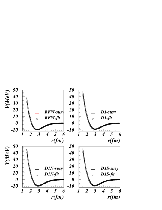
Figure 6: Gaussian expansion of the SUSY potentials. The fit was performed in a restricted radial range $r\sim 1.5-10fm$

Figure 7: The S-state phase shift calculated with fitted SUSY potentials.

Figure 8: The S-state resonance in ⁸Be calculated with fitted SUSY potentials. Resonance parameters lie in the experimental range [37] for all interactions.

In order to facilitate the calculation for $\alpha$-matter we expand the SUSY potentials in Gaussian form factors, similar to the Ali-Bodmer interaction,

$$V_{fit}(r)=V_{r}e^{-(\mu_{r}r)^{2}}-V_{a}e^{-(\mu_{a}r)^{2}}$$ (36)

with $V_{r},\mu_{r},V_{a},\mu_{a}$ fitting parameters. Since it is impossible to obtain meaningful parameters in the whole radial range, we restrict the fit in the relevant $r=(1.5-10)$ fm. The result is given in the Table 1. We obtain almost perfect fits, Fig (6), but comparison with experimental data require to repeat the renormalization procedure described above. The correction is of the order of $1\%$ in all cases.

Table 1: Parameters for the fitted SUSY potentials. The parameter $\lambda$ is a renormalization constant which gives the best fit for the experimental S-state phase shift and the $0^{+}$ resonance in ⁸Be.

Int	$V_{r}$(MeV)	$\mu_{r}$(fm-1)	$V_{a}$(MeV)	$\mu_{a}$(fm-1)	$\lambda$
BFW	254.8000031	0.6470000	101.9716263	0.4600000	0.9920
D1	255.8999939	0.6049346	103.6447830	0.4370000	0.9891
D1N	265.0000000	0.6266215	102.5655823	0.4459522	0.9873
D1S	262.0000000	0.6194427	103.4447250	0.4437624	0.9906

4 Concluding remarks

We have calculated the $\alpha-\alpha$ interaction potential within the double folding model using finite range density dependent NN effective interactions. The knock-on nonlocal kernel corresponding to the finite range components of the effective interaction is localized within the lowest order of the Perey-Saxon approximation at zero energy. The resulted folding potentials are deep with an average strength of $78\pm 7$ MeV very close to the value of Schmid and Wildermuth [5] in their RGM calculation. The $\it{rms}$ radius of these potentials is somewhat larger than the corresponding value of the phenomenological BFW potential (see Fig. 1). Our deep folding potentials reproduce quite well the experimental values of the S-state phase shift and the properties of the first $0^{+}$ resonance in ⁸Be. The maximum deviation from unity of the usual renormalization factor $\lambda$ is $9\%$.

Successive supersymmetric transformations which preserve the continuous spectrum are used to remove the redundant 0S and 1S states in order to obtain physically relevant potentials. The phase shift and the properties of the $0^{+}$ resonance are calculated with the variable phase equation of Calogero with proper boundary condition for singular potentials. A Gaussian expansion of the resulted SUSY potentials shows a well known molecular pocket with an almost unique long range attractive component with $\mu_{a}=0.442\pm 0.005$ fm^-1. The potential minimum is located at about r=3 fm, which corresponds to a touching configuration and therefore implies a very small overlap of the single particle densities.

We believe that our potentials are physically meaningful in the energy range $E_{lab}=0-5$ MeV. Beyond this range high $\ell$-order phase shift starts to have significant values.

5 Acknoledgements

This work was supported by UEFISCDI-ROMANIA under program PN-II contract No. 55/2011 and by French-Romanian collaboration IN2P3/IFIN-HH. M. L. thanks to the staff of DFT/IFIN-HH for the kind hospitality during the preparation of this work.

References

- [1] J. M. Lattimer, F. G. Sweety, Nucl. Phys. A535, 331 (1983).
- [2] F. Carstoiu and Ş. Mişicu, Phys. Lett. B682, 33 (2009).
- [3] S. A. Sofianos, R. M. Adam and V. B. Belyaev, Phys. Rev. C 84, 064311 (2011).
- [4] E. van der Spuy, Nucl. Phys. 11, 615 (1959).
- [5] E. W. Schmid and K. Wildermuth, Nucl. Phys. 26, 463 (1961).
- [6] B. Buck, H. Friedrich and C. Wheatley,Nucl. Phys. A275, 246 (1977).
- [7] S. Ali and A. R. Bodmer, Nucl. Phys. A80, 99 (1966).
- [8] K. Langanke, H. -M. Müller, Phys. Rep. 227, 647 (1993).
- [9] T. Yamada and P. Schuck, Phys. Rev. C 69, 024309 (2004).
- [10] S. A. Sofianos, K. C. Panda and P. E. Hogdson, J. Phys. G: Part. Phys. 19, 1929 (1993).
- [11] D. Baye, Phys. Rev. Lett. 58, 2738 (1987).
- [12] J. -M. Sparenberg and D. Baye, Phys. Rev. C 54, 1309 (1996).
- [13] F. Carstoiu and R. J. Lombard, Ann. Phys. (N.Y.) 217, 279 (1992).
- [14] D. Gogny, in Proc. Int. Conf. on Nuclear Physics, eds. J. De Boer and H. Mang (North-Holland, Amsterdam, 1973).
- [15] J. Dechargé and D. Gogny, Phys. Rev. C 21, 1568 (1980).
- [16] F. Chappert, M. Girod and S. Hilaire, Phys. Lett. B668, 420 (2009).
- [17] J. S. Al-Khalili, J. A. Tostevin and I. J. Thompson, Phys. Rev. C 54, 1843 (1996).
- [18] O. Bohigas and S. Stringari, Phys. Lett. 95B, 9 (1980).
- [19] M. Gaudin et et al., Nucl. Phys. A176, 237 (1971).
- [20] R. F. Frosch, J. S. McCarthy, R. E. Rand and M. R. Yearian, Phys. Rev. 160, 874 (1967).
- [21] X. Campi and D. W. L. Sprung, Nucl. Phys. A194, 401 (1972).
- [22] F. Duggan, M. Lassaut, F. Michel and N. Vinh-Mau, Nucl. Phys. A355, 141 (1981)
- [23] F. Carstoiu and M. Lassaut, Nucl. Phys. A597, 269 (1996).
- [24] R. E. Peierls and N. Vinh Mau, Nucl. Phys. A343, 1 (1980).
- [25] S.Misicu, private comm.
- [26] D. Baye, J. Phys A:Math Gen 20, 5529 (1987)
- [27] D. Baye and J. -M. Sparenberg, J. Phys A:Math Gen 37, (2004) 10223
- [28] L. U. Ancarani and D. Baye, Phys. Rev. A 46, 206 (1992).
- [29] D. Baye, Phys. Rev. A 48, 2040 (1993).
- [30] J. -M Sparenberg, D. Baye and H. Leeb, Phys. Rev. C 61, 024605 (2000)
- [31] R. G. Newton, Scattering Theory of Waves and Particles, (Springer, Berlin, 1982) 2nd ed.
- [32] K. Chadan and P.C. Sabatier, Inverse Problems in Quantum Scattering Theory (Springer, Berlin, 1989) 2nd ed.
- [33] F. Calogero, Variable Phase Approach to Potential Scattering, Academic Press, New York and London, (1967).
- [34] Erdélyi A, Magnus W, Oberhettinger F and Tricomi F G 1953 Higher Transcendental Functions vol II (New York: McGraw-Hill).
- [35] P. Swan, Nucl. Phys. 46, 669 (1963).
- [36] S. A. Afzal, A. A. Z. Ahmad and S. Ali, Rev. Mod. Phys. 41, 247 (1969).
- [37] J. Benn, E. B. Dally, H.H. Müller, R.E. Pixley, H. H. Staub and H. Winkler, Phys. Lett. 20, 43 (1966).
- [38] M. Lassaut, S.Y Larsen, S.A. Sofianos and S.A. Rakityansky, J. Phys. A: Math. Gen. 34, 2007 (2001).