Hierarchical block structures and high-resolution model selection in large networks

Abstract

Discovering and characterizing the large-scale topological features in empirical networks are crucial steps in understanding how complex systems function. However, most existing methods used to obtain the modular structure of networks suffer from serious problems, such as being oblivious to the statistical evidence supporting the discovered patterns, which results in the inability to separate actual structure from noise. In addition to this, one also observes a resolution limit on the size of communities, where smaller but well-defined clusters are not detectable when the network becomes large. This phenomenon occurs not only for the very popular approach of modularity optimization, which lacks built-in statistical validation, but also for more principled methods based on statistical inference and model selection, which do incorporate statistical validation in a formally correct way. Here we construct a nested generative model that, through a complete description of the entire network hierarchy at multiple scales, is capable of avoiding this limitation, and enables the detection of modular structure at levels far beyond those possible with current approaches. Even with this increased resolution, the method is based on the principle of parsimony, and is capable of separating signal from noise, and thus will not lead to the identification of spurious modules even on sparse networks. Furthermore, it fully generalizes other approaches in that it is not restricted to purely assortative mixing patterns, directed or undirected graphs, and ad hoc hierarchical structures such as binary trees. Despite its general character, the approach is tractable, and can be combined with advanced techniques of community detection to yield an efficient algorithm that scales well for very large networks.

I Introduction

The detection of communities and other large-scale structures in networks has become perhaps one of the largest undertakings in network science Newman (2011); Fortunato (2010). It is motivated by the desire to be able to characterize the most salient features in large biological Girvan and Newman (2002); Ravasz et al. (2002); Fletcher Jr et al. (2013), technological Albert et al. (1999); Yook et al. (2002) and social systems Girvan and Newman (2002); Zhao et al. (2011); Palla et al. (2005), such that their building blocks become evident, potentially giving valuable insight into the central aspects governing their function and evolution. At its simplest level, the problem seems straightforward: Modules are groups of nodes in the network that have a similar connectivity pattern, often assumed to be assortative, i.e., connected mostly among themselves and less so with the rest of the network. However, when attempting to formalize this notion, and develop methods to detect such structures, the combined effort of many researchers in recent years has spawned a great variety of competing approaches to the problem, with no clear, universally accepted outcome Fortunato (2010).

The method that has perhaps gathered the most widespread use is called modularity optimization Newman and Girvan (2004) and consists in maximizing a quality function that favors partitions of nodes for which the fraction of internal edges inside each cluster is larger than expected given a null model, taken to be a random graph. This method is relatively easy to use and comprehend, works well in many accessible examples, and is capable of being applied in very large systems via efficient heuristics Clauset et al. (2004); Blondel et al. (2008). However it also suffers from serious drawbacks. In particular, despite measuring a deviation from a null model, it does not take into account the statistical evidence associated with this deviation, and as a result it is incapable of separating actual structure from those arising simply of statistical fluctuations of the null model, and it even finds high-scoring partitions in fully random graphs Guimerà et al. (2004). This problem is not specific to modularity and is a characteristic shared by the vast majority of methods proposed for solving the same task Fortunato (2010). In addition to the lack of statistical validation, modularity maximization fails to detect clusters with size below a given threshold Fortunato and Barthélemy (2007); Lancichinetti and Fortunato (2011), which increases with the size of the system as $\sim\sqrt{E}$, where $E$ is the number of edges in the entire network. This limitation is independent of how salient these relatively smaller structures are, and makes this potentially very important information completely inaccessible. Furthermore, results obtained with this method tend to be degenerate for large empirical networks Good et al. (2010), for which many different partitions can be found with modularity values very close to the global maximum. In these common situations, the method fails in giving a faithful representation of the actual large-scale structure present in the system.

More recently, increasing effort has been spent on a different approach based on the statistical inference of generative models, which encodea the modular structure of the network as model parameters Hastings (2006); Garlaschelli and Loffredo (2008); Newman and Leicht (2007); Reichardt and White (2007); Hofman and Wiggins (2008); Bickel and Chen (2009); Guimerà and Sales-Pardo (2009); Karrer and Newman (2011); Ball et al. (2011); Reichardt et al. (2011); Zhu et al. (2014); Baskerville et al. (2011). This approach offers several advantages over a dominating fraction of existing methods, since it is more firmly grounded on well-known principles and methods of statistical analysis, which allows the incorporation of the statistical evidence present in the data in a formally correct manner. Under this general framework, one could hope to overcome some of the limitations existing in more ad hoc methods, or at least make any intrinsic limitations easier to understand in light of more robust concepts Decelle et al. (2011a, b); Mossel et al. (2012); Peixoto (2013a). The generative model most used for this purpose is the stochastic block model Holland et al. (1983); Fienberg et al. (1985); Faust and Wasserman (1992); Anderson et al. (1992); Hastings (2006); Garlaschelli and Loffredo (2008); Newman and Leicht (2007); Reichardt and White (2007); Hofman and Wiggins (2008); Bickel and Chen (2009); Guimerà and Sales-Pardo (2009); Karrer and Newman (2011); Ball et al. (2011); Reichardt et al. (2011); Zhu et al. (2014); Baskerville et al. (2011), which groups nodes in blocks with arbitrary probabilities of connections between them. This very simple definition already does away with the restriction of considering only purely assortative communities, and accommodates many different patterns, such as core-periphery structures and bipartite blocks, as well as straightforward generalizations to directed graphs. In this context, the detectability of well-defined clusters amounts, in large part, to the issue of model selection based on principled criteria such as minimum description length (MDL) Rosvall and Bergstrom (2007); Peixoto (2013a) or Bayesian model selection (BMS) Daudin et al. (2008); Mariadassou et al. (2010); Moore et al. (2011); Latouche et al. (2012); Côme and Latouche (2013). These approaches allow the selection of the most appropriate number of blocks based on statistical evidence, and thus avoid the detection of spurious communities. However, frustratingly, at least one of the limitations of modularity maximization is also present when doing model selection, namely, the resolution limit mentioned above. As was recently shown in Ref. Peixoto (2013a), when using MDL, the maximum number of detectable blocks scales with $\sqrt{N}$, where $N$ is the number of nodes in the network, which is very similar to the modularity optimization limit. However, in this context, this limitation arises out of the lack of knowledge about the type of modular structure one is about to infer, and the a priori assumption that all possibilities should occur with the same probability. Here we develop a more refined method of model selection, which consists in a nested hierarchy of stochastic block models, where an upper level of the hierarchy serves as prior information to a lower level. This dramatically changes the resolution of the model selection procedure, and replaces the characteristic block size of $\sqrt{N}$ in the nonhierarchical model by much a smaller value that scales only logarithmically with $N$, enabling the detection of much smaller blocks in very large networks. Furthermore, the approach provides a description of the network in many scales, in a complete model encapsulating its entire hierarchical structure at once. It generalizes previous methods of hierarchical community detection Clauset et al. (2007, 2008); Rosvall and Bergstrom (2011); Sales-Pardo et al. (2007); Ronhovde and Nussinov (2009); Kovács et al. (2010); Park et al. (2010), in that it does not impose specific patterns such as dendograms or binary trees, in addition to allowing arbitrary modular structures as the usual stochastic block model, instead of purely assortative ones. Furthermore, despite its increased resolution, the approach attempts to find the simplest possible model that fits the data, and is not subject to overfitting, and, hence, will not detect spurious modules in random networks. Finally, the method is fully nonparametric, and can be implemented efficiently, with a simple algorithm that scales well for very large networks.

In Sec. II, we start with the definition of the model and then we discuss the model-selection procedure based on MDL. We then move to the analysis of the resolution limit, and proceed to define an efficient algorithm for the inference of the nested model, and we finalize with the analysis of synthetic and empirical networks, where we demonstrate the quality of the approach. We then conclude with an overall discussion.

II Hierarchical Model

The original stochastic block model ensemble Holland et al. (1983); Fienberg et al. (1985); Faust and Wasserman (1992); Anderson et al. (1992) is composed of $N$ nodes, divided into $B$ blocks, with $e_{rs}$ edges between nodes of blocks $r$ and $s$ (or, for convenience of notation, twice that number if $r=s$). Here, we differentiate between two very similar model variants: 1. the edge counts $e_{rs}$ are themselves the parameters of the model; 2. the parameters are the probabilities $p_{rs}$ that an edge exists between two nodes of the respective blocks, such that the edge counts ${\left<e_{rs}\right>}=n_{r}n_{s}p_{rs}$ are constrained on average. Both are equally valid generative models, and as long as the edge counts are sufficiently large, they are fully equivalent (see Ref. Peixoto (2012) and Appendix A). Here, we stick with the first variant, since it makes the following formulation more convenient. We also consider a further variation called the degree-corrected block model Karrer and Newman (2011), which is defined exactly as the traditional model(s) above, but one additionally specifies the degree sequence $\{k_{i}\}$ of the graph as an additional set of parameters (again, these values can be the parameters themselves, or they can be constrained on average Peixoto (2012)). The degree-corrected version, although it is a relatively simple modification, yields much more convincing results on many empirical networks, since it is capable of incorporating degree variability inside each block Karrer and Newman (2011). As will be seen below, it is, in general, also capable of providing a more compact description of arbitrary networks than the traditional version.

The nested version, which we define, here is based on the simple fact that the edge counts $e_{rs}$ themselves form a block multigraph, where the nodes are the blocks, and the edge counts are the edge multiplicities between each node pair (with self-loops allowed). This multigraph may also be constructed via a generative model of its own. If we choose a stochastic block model again as a generative model, we obtain another smaller block multigraph as parameters at a higher level, and so on recursively, until we finally reach a model with only one block. This forms a nested stochastic block model hierarchy, which describes a given network at several resolution levels (see Fig. 1).

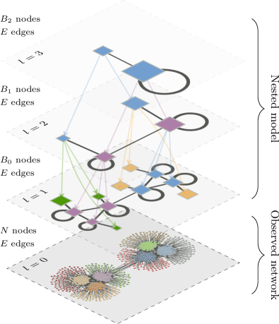
Figure 1: Example of a nested stochastic block model with three levels, and a generated network at the bottom. The top-level structure describes a core-periphery network, which is further subdivided in the lower levels.

This approach provides an increased resolution when performing model selection, since the generative model inferred at an upper level serves as prior information to the one at a lower level. Despite its more elaborate formulation, this hierarchical model remains tractable, and it is possible to apply it to very large networks, in a fully nonparametric manner, as discussed below. Furthermore, it generalizes cleanly the flat variants, which correspond simply to a hierarchy with only one level. It also does not impose any preferred mixing pattern (e.g., assortative or dissortative block structures), and is not restricted to any specific hierarchical form, such as binary trees or dendograms. In the following, we describe the maximum likelihood method to infer the multilevel partitions, and the model selection process based on the minimum description length principle, and compare it with Bayesian model selection.

In the analysis, we focus on undirected networks, but everything is straightforwardly applicable to directed networks as well. In Appendix C we present a summary of the relevant expressions for the directed case.

II.1 Module inference

The inference approach consists in finding the best partition $\{b_{i}\}$ of the nodes, where $b_{i}\in[1,B]$ is the block membership of node $i$, in the observed network $G$, such that the posterior likelihood $\mathcal{P}(G|\{b_{i}\})$ is maximized. Since each graph with the same edge counts $e_{rs}$ occurs with the same probability, the posterior likelihood is simply $\mathcal{P}(G|\{b_{i}\})=1/\Omega(\{e_{rs}\},\{n_{r}\})$, where $e_{rs}$ and $n_{r}$ are the edge and node counts associated with the block partition $\{b_{i}\}$, and $\Omega(\{e_{rs}\},\{n_{r}\})$ is the number of different network realizations. Hence, maximizing the likelihood is identical to minimizing the ensemble entropy Peixoto (2012); Bianconi (2009) $\mathcal{S}(\{e_{rs}\},\{n_{r}\})=\ln\Omega(\{e_{rs}\},\{n_{r}\})$.

For the lowest level of the hierarchy (which models directly the observed network), we have a simple graph, for which the entropies can be computed as Peixoto (2012)

$$\mathcal{S}_{t}=\frac{1}{2}\sum_{rs}n_{r}n_{s}H_{\text{b}}\left(\frac{e_{rs}}{n_{r}n_{s}}\right),$$ (1)

for the traditional block model ensemble and,

$$\mathcal{S}_{c}\simeq-E-\sum_{k}N_{k}\ln k!-\frac{1}{2}\sum_{rs}e_{rs}\ln\left(\frac{e_{rs}}{e_{r}e_{s}}\right),$$ (2)

for the degree-corrected variant, where $E=\sum_{rs}e_{rs}/2$ is the total number of edges, $N_{k}$ is the total number of nodes with degree $k$, $e_{r}=\sum_{s}e_{rs}$ is the number of half-edges incident on block $r$, $H_{\text{b}}(x)=-x\ln x-(1-x)\ln(1-x)$ is the binary entropy function, and it was assumed that $n_{r}\gg 1$. Note that only the last term of Eq. 2 is, in fact, useful when finding the best block partition, since the other terms remain constant. However the full expression is necessary when comparing the models against each other via model selection, as discussed below.

For the upper-level multigraphs the entropy can also be computed Peixoto (2012), and it takes a different form

$$\mathcal{S}_{m}=\sum_{r>s}\ln{\textstyle\left(\kern-3.00003pt\left(\genfrac{}{}{0.0pt}{}{n_{r}n_{s}}{e_{rs}}\right)\kern-3.00003pt\right)}+\sum_{r}\ln{\textstyle\left(\kern-3.00003pt\left(\genfrac{}{}{0.0pt}{}{\left(\kern-2.10002pt\left(\genfrac{}{}{0.0pt}{}{n_{r}}{2}\right)\kern-2.10002pt\right)}{e_{rr}/2}\right)\kern-3.00003pt\right)},$$ (3)

where $\left(\kern-3.00003pt\left(\genfrac{}{}{0.0pt}{}{n}{m}\right)\kern-3.00003pt\right)={n+m-1\choose m}$ is the number of $m$-combinations with repetitions from a set of size $n$. Note that we no longer assume that $n_{r}\gg 1$, since at the upper levels the number of nodes becomes arbitrarily small.

At each level $l\in[0,L]$ in the hierarchy there are $B_{l-1}$ nodes, which are divided into $B_{l}$ blocks (with $B_{l}\leq B_{l-1}$), were we set $B_{-1}\equiv N$. The edge counts at level $l$ are denoted $e^{l}_{rs}$, and the block sizes $n^{l}_{r}$. Therefore, we must have that $\sum_{r}n^{l}_{r}=B_{l-1}$ and $\sum_{rs}e_{rs}^{l}/2=E$; i.e., the total number of nodes decreases in the upper levels, but the total number of edges remains the same. The combined entropy of all layers is then given by

$$\mathcal{S}_{n}=\mathcal{S}_{t/c}(\{e^{0}_{rs}\},\{n^{0}_{r}\})+\sum_{l=1}^{L}S_{m}(\{e^{l}_{rs}\},\{n^{l}_{r}\}).$$ (4)

The full generative model corresponds to a nested sequence of network ensembles, where each sample from a given level generates another ensemble at a lower level. The entropy in Eq. 4 represents the amount of information necessary to encode the decision sequence, which, starting from the topmost model, selects the observed network among all possible branches in the lower levels.

Whenever both the number of levels and the number of blocks $B_{l}$ of each level is known, the best multilevel partition is the one that minimizes $\mathcal{S}_{n}$. However, such information regarding the size of the model is most often not available, and needs to be inferred from the data as well. Using Eq. 4 for this purpose is not appropriate, since minimizing it across all possible hierarchies leads to a trivial and meaningless result where $B_{l}=N$ for all $l$. Instead, one must employ some form of Occam’s razor and select the simplest possible model that best describes the observed data without increasing its complexity. We present such an approach in the next section.

II.2 Model selection

A method that directly formalizes Occam’s razor principle is known as minimum description length Grünwald (2007); Rissanen (2010), where one specifies the total amount of information necessary to described the data, which includes not only the sample but the model parameters as well. The description length for the model above is

$$\Sigma=\mathcal{L}_{t/c}+\mathcal{S}_{t/c},$$ (5)

where $\mathcal{L}_{t/c}$ is the amount of information necessary to fully describe the model, and $\mathcal{S}_{t/c}$ corresponds to entropy of the lowest level $l=0$ of the hierarchy. In a given level $l$ of the hierarchy, the information required to describe the model parameters $\{e^{l}_{rs}\}$ is given by the entropy $S_{m}$ (Eq. 3) of the model in level $l+1$, so that we may write

$$\mathcal{L}_{t}=\sum_{l=1}^{L}S_{m}(\{e^{l}_{rs}\},\{n^{l}_{r}\})+\mathcal{L}^{l-1}_{t}.$$ (6)

The only missing information is how to partition the nodes of the current level into $B_{l}$ blocks, which corresponds to the term $\mathcal{L}^{l}_{t}$ in the equation above. The total number of partitions with the same block sizes $\{n_{r}^{l}\}$ is given by $B_{l-1}!/\prod_{r}n_{r}^{l}!$, and the total number of different block sizes is $\left(\kern-3.00003pt\left(\genfrac{}{}{0.0pt}{}{B_{l}}{B_{l-1}}\right)\kern-3.00003pt\right)$. Hence, the amount of information necessary to describe the block partition of level $l$ is

$$\mathcal{L}^{l}_{t}=\ln{\textstyle\left(\kern-3.00003pt\left(\genfrac{}{}{0.0pt}{}{B_{l}}{B_{l-1}}\right)\kern-3.00003pt\right)}+\ln B_{l-1}!-\sum_{r}\ln n_{r}^{l}!.$$ (7)

Note that this is different from the choice made in Refs. Peixoto (2013a); Rosvall and Bergstrom (2007), which considered all possible $B_{l}^{B_{l-1}}$ partitions to be equally likely, and, hence, computed the necessary amount of information as $B_{l-1}\ln B_{l}$. This choice implicitly assumes that all blocks have approximately equal sizes, and offers a worse description when this is not the case. Note that for $B_{l-1}\gg 1$, we have

$$\mathcal{L}^{l}_{t}\simeq B_{l-1}H(\{n_{r}^{l}/B_{l-1}\}),$$ (8)

where $H(\{p_{i}\})=-\sum_{i}p_{i}\ln p_{i}$ is the entropy of the distribution $\{p_{i}\}$. Therefore, for uniform blocks $n^{l}_{r}=B_{l-1}/B_{l}$ we recover asymptotically the value $\mathcal{L}^{l}_{t}\simeq B_{l-1}\ln B_{l}$. However, the value of Eq. 7 can be much smaller for nonuniform partitions. This choice has important consequences for the resolution of relatively small blocks, as will be seen below.

For the degree-corrected version, we still need to include the information necessary to describe the degrees at the lowest level,

$$\mathcal{L}_{c}=\mathcal{L}_{t}+\sum_{r}n_{r}H(\{p^{r}_{k}\}),$$ (9)

where $\{p^{r}_{k}\}$ is the degree distribution of nodes belonging to block $r$ . It is worth noting that, if a network is sampled from the traditional block model ensemble, so that $p_{k}^{r}$ is a Poisson with average $e_{r}/n_{r}$, Eq. 9 becomes $\mathcal{L}_{c}=\mathcal{L}_{t}+2E-\sum_{r}e_{r}\ln e_{r}/n_{r}+\sum_{k}N_{k}\ln k!$, which means that $\mathcal{S}_{c}+\mathcal{L}_{c}=\mathcal{S}_{t}+\mathcal{L}_{t}$, i.e. the total description length is identical for both the traditional and degree-corrected models in this case, and, therefore, both models describe the same network equally well. However, if the distributions $\{p^{r}_{k}\}$ deviate from Poissons, the degree-corrected variant will provide, in general, a shorter description length.

It is easy to see that if one has a flat $L=1$ hierarchy, with $\{B_{l}\}=\{B,1\}$, the description length of the nonhierarchical model is recovered Peixoto (2013a); e.g., for the traditional model, we have $\Sigma_{L=1}=\mathcal{L}_{L=1}+\mathcal{S}_{t},$ with

$$\mathcal{L}_{L=1}=\ln{\textstyle\left(\kern-3.00003pt\left(\genfrac{}{}{0.0pt}{}{\left(\kern-2.10002pt\left(\genfrac{}{}{0.0pt}{}{B}{2}\right)\kern-2.10002pt\right)}{E}\right)\kern-3.00003pt\right)}+\ln{\textstyle\left(\kern-3.00003pt\left(\genfrac{}{}{0.0pt}{}{B}{N}\right)\kern-3.00003pt\right)}+\ln N!-\sum_{r}\ln n_{r}!,$$ (10)

where the only difference in comparison to Ref. Peixoto (2013a) is that here we are using the improved partition description length of Eq. 7. Therefore, the nested generalization fully encapsulates the flat version, such that $\min\Sigma\leq\min\Sigma_{L=1}$; i.e., the nested model can provide only a shorter or equal description length of the observed network.

The MDL principle predicates that whenever the hierarchy itself needs to be inferred, one should minimize Eq. 5, instead of Eq. 4 directly. However, MDL is one of the many principled methods one could use to do model selection, which include, e.g., Bayesian model selection via integrated likelihood Biernacki et al. (2000); Hofman and Wiggins (2008); Daudin et al. (2008); Mariadassou et al. (2010); Latouche et al. (2012); Côme and Latouche (2013), likelihood ratios Yan et al. (2012) or more approximative methods such as Bayesian information criterion (BIC) Schwarz (1978) and Akaike information criterion (AIC) Akaike (1974). If any two of these methods are derived from equivalent assumptions, one should expect them to deliver compatible results. In Appendix A we make a comparison of the MDL approach with Bayesian model selection via integrated likelihood (BMS), since it is nonapproximative and can be computed exactly for the stochastic block model, where we show that under compatible assumptions, these two methods deliver the exact same results. In the following, we compare the results obtained with nonhierarchical MDL/BMS and the nested model presented, and show that it yields a higher quality model selection criterion, which detects the correct number of blocks for sparse networks, without being overconfident. Based on this analysis we are capable of deriving the optimum number of blocks given a network size, and we show that the nested model does not suffer from the resolution limit, which hinders the nonhierarchical approach.

II.2.1 Module detectability and the “resolution limit”

The general problem of module detectability can be formulated as follows: Suppose we generate a network with a given parameter set. To what extent can we recover the planted parameters by observing this single sample from the model? The answer is conditional on the amount of one’s prior knowledge. If the number of blocks $B$ is known beforehand, the remaining task is simply to classify the nodes in one of these $B$ classes. This problem has been shown to exhibit a detectability-indetectability phase transition Decelle et al. (2011a, b); Reichardt and Leone (2007); Hu et al. (2012): If the existing block structure is too weak, it becomes impossible to infer the correct partition with any method, despite the fact that the model parameters deviate from that of a fully random graph. On the other hand, if the block structure is sufficiently strong, it is possible to detect the correct partition with a precision that increases as the block structure becomes stronger. Another situation is when one does not know the correct number $B$, which is arguably more relevant in practice. In this case, in addition to the node classification, one needs to perform model selection. Ideally, one would like to find the correct $B$ value whenever the corresponding partition is detectable. However, in situations where the correct partition is only partially detectable, i.e., the inferred partition is positively but weakly correlated with the true model, an application of Occam’s razor may actually choose a simpler model, with smaller $B$, with a comparable correlation with the true partition. Hence, if we lack knowledge of the model size $B$, there will be situations where the true partition will be more poorly detected, when compared to the case where we have this information. This can be clearly illustrated with a very simple example known as the planted partition (PP) model Condon and Karp (2001). It corresponds to an assortative block structure given by $e_{rs}=2E[\delta_{rs}c/B+(1-\delta_{rs})(1-c)/B(B-1)]$, $n_{r}=N/B$, and $c\in[0,1]$ is a free parameter that controls the assortativity strength. For this model, if we have that $N/B\gg 1$, it can be shown that the detectable phase exists for ${\left<k\right>}>[(B-1)/(cB-1)]^{2}$ Decelle et al. (2011a, b); Mossel et al. (2012). Let us make the situation even simpler and consider the strongest possible block structure with $c=1$, i.e. $B$ perfectly isolated assortative communities with $N/B$ nodes. In this case the detectability threshold lies at ${\left<k\right>}=1$. Therefore, for any ${\left<k\right>}>1$, we should be able to detect all $B$ blocks, with a precision increasing with ${\left<k\right>}$, if we know we have $B$ blocks to begin with. If we do not know this, we must apply a model-selection criterion as described above to obtain the best value of $B$. For simplicity, let us assume that, for the correct value of $B\equiv B_{\text{true}}$ the true partition is perfectly detected, such that $\mathcal{S}_{t}\simeq-E\ln B$, ignoring additive constants, which are irrelevant at this point. If a value of $B>B_{\text{true}}$ is used, we assume that the inferred partition corresponds to regular subdivisions of the planted one, such that the entropy remains approximately unchanged $\mathcal{S}_{t}\simeq-E\ln B_{\text{true}}$. For $B<B_{\text{true}}$, the blocks are uniformly merged together, so that $\mathcal{S}_{t}\simeq-E\ln B$. Hence, we may write the expected value of the minimum description length in the nonhierarchical model by summing $\mathcal{S}_{t}=-E\ln\min(B,B_{\text{true}})$ with Eq. 10. For the nested version of the model, we assume a regular hierarchy tree of depth $L$ and with a fixed branching ratio $\sigma$, i.e. $B_{l}=\sigma^{L-l}$, so that Eq. 5 becomes

$$\Sigma\simeq\left(\kern-3.00003pt\left(\genfrac{}{}{0.0pt}{}{\sigma}{2}\right)\kern-3.00003pt\right)\frac{B}{\sigma-1}\ln E+\frac{\sigma}{2}B\ln B+N\ln B\\ -E\ln\min(B,B_{\text{true}}),$$ (11)

where $B_{l}\gg\sigma$ was assumed, together with $L\gg 1$, and $B\equiv B_{0}$. One may compare these criteria against each other in their capacity of recovering the planted value of $B$, by finding the extremum of each function. In Fig. 2, we show the optimum values of $B$ for a model with $N=10^{4}$ and $B_{\text{true}}=100$, as well as the results for the direct minimization of the corresponding exact quantities for actual network realizations, and a comparison of the obtained partitions using the normalized mutual information (NMI). We also include the comparison with a dense BMS criterion (see Appendix A) both in its full form (Eqs. 17 and 20), and with the partition likelihood term omitted, i.e. $\mathcal{P}(\{b_{i}\}|B)=1$ in Eq. 17, as was done in Refs. Guimerà and Sales-Pardo (2009); Moore et al. (2011). We see that the dense BMS criterion fails to detect the correct model size for sparser networks, which is in accordance with its inadequacy in this region. The hierarchical model provides, as expected, the best results, and detects the correct model for the sparsest networks. The incomplete BMS criterion is clearly overconfident for sparse networks, and detects $B>1$ structures even when the model lies below the detectability threshold ${\left<k\right>}=1$; hence, this shows that the partition likelihood should not simply be discarded. Both MDL and dense BMS fail to detect anything for ${\left<k\right>}<2$, which corresponds to a strong threshold, which interestingly lies above the strict detectability limit at ${\left<k\right>}=1$. This corresponds to a region where detectability is possible, but only if the true value of $B$ is known (or if a more refined model-selection criterion exists). Note that the incomplete BMS criterion performs better in the region $1<{\left<k\right>}<2$, but this is perhaps better interpreted as a by-product of its overall overconfidence for very sparse networks. Note that all criteria eventually agree on the correct value if ${\left<k\right>}$ is made sufficiently large, which corresponds to the intuitive notion that the detection problem becomes much easier for dense networks.

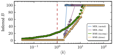
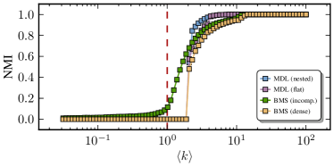
Figure 2: Model selection results for a PP model with $N=10^{4}$, $B_{\text{true}}=100$ and fully isolated blocks ($c=1$), using the model selection criteria described in the text. The top panel shows the inferred value of $B$ versus the average degree ${\left<k\right>}$ in the network. The solid lines show the theoretical value according to each criterion, and the data points are direct optimization of the corresponding quantities for actual generated network, averaged over $40$ independent realizations. The bottom panel shows the normalized mutual information (NMI) between the inferred and planted partitions. The dashed line marks the threshold ${\left<k\right>}=1$ where inference becomes impossible for $N\to\infty$.

A prominent problem in the detectability of block structures via other methods, such as modularity optimization Newman and Girvan (2004) is when modules are merged together, regardless of how strong the community structure is perceived to be. For the modularity-based approach, when considering a maximally modular network, similar to the PP model with $c\to 1$, but with the additional restriction that the graph remains connected, it has been shown Fortunato and Barthélemy (2007) that modules are merged together as long as $B>\sqrt{E}$. This phenomenon is considered counterintuitive, and has been called the “resolution limit” of community detection via this method. As it happens, this problem does not only occur for modularity-based methods, but also if one does statistical inference based on MDL. For the nonhierarchical model, it can be shown that, according to this criterion, the optimal number of blocks scales as $B^{*}\simeq\mu({\left<k\right>})\sqrt{N}$, where $\mu(x)$ is an increasing function Peixoto (2013a). Therefore if the planted number exceeds this threshold, blocks will be merged together, despite the fact that the block structure is detectable with arbitrary precision if one knows the correct value of $B$, and it sufficiently exceeds the detectability threshold ${\left<k\right>}>1$ of the PP model. This means that the true parameters of the model can no longer be used to compress the generated data. This is a direct result of the assumption that all possible block structures of a given size are equally possible, and the number of such models becomes very large, with a model description length scaling roughly with $\sim B^{2}\ln E+N\ln B$. In the presence of additional assumptions about the model, such as the fact that one is dealing with the PP model, instead of a more general block structure, this can, in principle, be improved. However, in most practical situations such assumptions cannot be made. One main advantage of the nested model is that this limit can be overcome without requiring such prior knowledge. The description length via the nested model for the maximally modular network above is given by Eq. 11 with $B_{\text{true}}=B$. As can be seen, this equation has only log-linear dependencies on the model size $B$, instead of the quadratic one present in the flat MDL. The result of this is that, if one finds the value of $B^{*}$, which minimizes the nested description length, one obtains the scaling

$$B^{*}\propto\frac{N}{\ln N},$$ (12)

for sufficiently large $N$. This is a significant improvement, since the maximum number of detectable blocks grows almost linearly with the number of nodes. Thus, a characteristic detectable block size $N/B^{*}\sim\sqrt{N}$ is replaced by a much smaller value $N/B^{*}\sim\ln N$, which allows for a precise assessment of small communities even in very large networks.

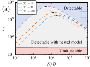
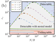
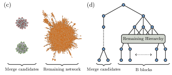
Figure 3: Parameter region where two isolated blocks with $e_{c}/2$ internal edges and $n_{c}=e_{c}/5$ internal nodes are detectable as separate blocks [shown schematically in panel (c)], as a function of the average block size $N/B$, and depending on (a) the average degree ${\left<k\right>}$ with $N=10^{5}$ and (b) the number of nodes $N$ with ${\left<k\right>}=20$. The dashed curves show the boundaries for the nonhierarchical block model, and the solid lines for the hierarchical variant. The line segments on the right-hand side of the plots show the detectability threshold for modularity Fortunato and Barthélemy (2007), $e_{c}^{*}=\sqrt{2E}$. The points marked with stars ($\star$) correspond to the maximum value of $B$ that is detectable in the remaining network with the nonhierarchical model, and the dotted line shows the same quantity for various ${\left<k\right>}$ values (i.e. the region on the left of this curve corresponds to an overfitting of the remaining network, according to the nonhierarchical criterion). (d) The hierarchical construction used to decide if the two isolated blocks are merged together with the nested model.

It is possible to understand in more detail the origin of the improvement by considering a related problem, which is the detection of specific blocks that are much smaller than the remaining network. Another facet of the resolution limit manifests itself when two such blocks are merged together, despite the fact that if they are considered in isolation they would be kept separate. Here, we consider this problem by using a slightly modified scenario than the one proposed in Ref. Fortunato and Barthélemy (2007), which is a network composed of two fully isolated blocks, each with $e_{c}/2$ internal edges and $n_{c}$ nodes, and a remaining network with $N$ nodes, $E$ edges, average degree ${\left<k\right>}=2E/N$ and an arbitrary topology [see Fig. 3(c)]. We may decide if these blocks are merged together by considering the difference in the description length. The entropy difference for the merge is simply $\Delta\mathcal{S}_{t}=e_{c}\ln 2$ (where we assume $e_{c}\ll n_{c}^{2}$, but the dense case can be computed as well, with no significant difference in the result). For the flat block model we have $\Delta\mathcal{L}_{\text{flat}}=\mathcal{L}_{L=1}(E+e_{c},N+2n_{c},B-1,\{n_{r}\}\cup\{2n_{c}\})-\mathcal{L}_{L=1}(E+e_{c},N+2n_{c},B,\{n_{r}\}\cup\{n_{c},n_{c}\})$, computed using Eq. 10. For this case, the point at which the merge happens, $\Delta\mathcal{L}_{\text{flat}}+\Delta\mathcal{S}_{t}=0$, will depend not only on the values of $E$ and $N$, but also on the average block size $N/B$ of the remaining network, as can be seen in Fig. 3(a) and (b). As the number of blocks in the remaining network approaches the maximum detectable value, $B^{*}\sim\sqrt{N}$, the more difficult it becomes to resolve the smaller blocks. The detectable region recedes further with increasing ${\left<k\right>}$, and also with the number of nodes in the remaining network as $e_{c}^{*}\sim\sqrt{N}$. Hence, the denser or larger the remaining network, the harder it becomes to detect the smaller blocks with the flat variant of the model. In Fig. 3 are also shown the values of $e_{r}^{*}$ for which modularity also fails to separate the blocks (if one considers that they are connected to themselves and to the rest of the network by single edges), which are overall compatible with the flat MDL criterion. The situation changes significantly with the nested model. To consider the merge, we assume an optimal block hierarchy which splits at the top into two branches, the left one containing the two smaller blocks, and the right one containing the remaining network and its arbitrary hierarchical structure [see Fig. 3(d)]. To consider the merge, we need to compute the description length only at the lowest level $l=0$, since the rest remains unchanged after the merge. By computing the difference via Eq. 5, after some manipulations we obtain $\Delta\Sigma_{\text{nested}}=\Delta\mathcal{S}_{t}+\ln n_{c}-\ln\left(\kern-3.00003pt\left(\genfrac{}{}{0.0pt}{}{3}{e_{c}}\right)\kern-3.00003pt\right)+\ln(B+1)-\ln(B+N-1)-\ln(B_{1}+B+2)$, with $B=B_{0}$. Note that this expression is independent of $E$, and, hence, the density of the remaining network cannot influence the merging decision. Since $B_{1}\leq B$, and assuming $B\gg 1$, we obtain $\Delta\Sigma_{\text{nested}}\simeq\Delta\mathcal{S}_{t}+\ln n_{c}-\ln[(e_{c}+2)(e_{c}+1)]-\ln(B+N)$, and, hence, the dependence on either $N$ or $B$ is again only logarithmic, $e^{*}_{c}\approx[\ln(B+N)-\ln n_{c}]/\ln 2$, as shown in Fig. 3(b). With this example one can notice that the nested model is capable of compartmentalizing the network at the upper levels, such that the lower-level branches can become almost independent of each other. This means that, in many practical situations, one can sufficiently overcome the resolution limit, without abandoning a global model that describes the whole network at once.

In the following section we specify an efficient algorithm to infer the parameters of the nested block model in arbitrary networks, and we test its efficacy in uncovering the multilevel structure of synthetic as well as empirical networks.

III Inference Algorithm

Individually, any specific level $l$ of the hierarchical structure is a regular block model, and, hence, the classification of the $B_{l-1}$ nodes of this level into $B_{l}$ blocks can be done via well-established methods, such as the Monte Carlo method Moore et al. (2011); Peixoto (2013a), simulated annealing, or belief propagation Decelle et al. (2011a, b); Yan et al. (2012). Here, we use the method described in Ref. Peixoto (2014), which is an agglomerative heuristic that provides high-quality results, while being unbiased with respect to the types of block structure that are inferred, and is also very efficient, with an algorithmic complexity of $O(N\ln^{2}N)$, independent of the number of blocks $B$. If one knows the depth $L$ of the hierarchy, and all $\{B_{l}\}$ values, the multilevel partitions can be obtained by starting from the lowest level $l=0$, and progressing upwards to $l=L$. However, this cannot be done when the number and sizes of the hierarchical levels are unknown. Although it is relatively simple to heuristically impose such patterns as binary trees or dendograms, these are not satisfactory given the general character of the model, which accommodates arbitrary branching patterns. However, traversing all possible hierarchies is not feasible for moderate or large networks; thus, one must settle with approximative methods. Here, we propose a very simple greedy heuristic, which, given any starting hierarchy, performs a series of local moves to obtain the optimal branching. Although this algorithm is not guaranteed to find the global optimum, we have found it to perform very well for many synthetic and empirical networks, and it tends to find consistent hierarchies, independently of the starting estimate. It is also efficient enough to allow its application to very large networks, since it does not significantly change the overall algorithmic complexity of the inference procedure. The algorithm is based on the following local moves at a given hierarchy level $l$:

1. Resize. A new partition of the $B_{l-1}$ nodes into a newly chosen number of blocks $B_{l}$ is obtained. This is done via the agglomerative heuristic mentioned previously, with the modification that it must not invalidate the partition at the level $l+1$; i.e., no nodes that belong to different blocks at the upper level can be merged together in the current level. This restriction enables the difference in $\Sigma$ (Eq. 5) to be computed easily, since it depends only on the modifications made in the current and upper levels, $l$ and $l+1$. The actual new value of $B_{l}$ is chosen via progressive bisection of the range $B_{l}\in[B_{l-1},B_{l+1}]$, so that the minimum of $\Sigma$ is bracketed, and for each value of $B_{l}$ attempted, the best partition is found with the algorithm of Ref. Peixoto (2014).

2. Insert. A new level is inserted at position $l$. Its size and partition are chosen exactly as in the resize move above.

3. Delete. The model in level $l$ is removed from the hierarchy; i.e., the nodes of level $l-1$ are grouped together directly as described in level $l+1$.

Through repeated applications of these moves, it is possible to construct any hierarchy. The actual greedy optimization consists of starting with some initial hierarchy and keeping track of whether or not each level is “done” or “not done.” One marks initially all levels as not done and starts at the top level $l=L$. For the current level $l$, if it is marked done it is skipped and one moves to the level $l-1$. Otherwise, all three moves are attempted. If any of the moves succeeds in decreasing the description length $\Sigma$, one marks the levels $l-1$ and $l+1$ (if they exist) as not done, the level $l$ as done, and one proceeds (if possible) to the upper level $l+1$, and repeats the procedure. If no improvement is possible, the level $l$ is marked as done and one proceeds to the lower level $l-1$. If the lowest level $l=0$ is reached and cannot be improved, the algorithm ends. Note that, in order to keep the description length complete, we must impose that $B_{L}=1$ throughout the above process. The final hierarchy will, in general, depend on the starting hierarchy, and as was mentioned above one cannot guarantee that the global minimum is always found. However, we find that, in the majority of cases, this algorithm succeeds in finding the same or very similar hierarchies, independently of the initial choice, which can simply be $\{B_{l}\}=\{1\}$. However, the actual time it takes to reach the optimum will depend on how close the initial tree was to the final one, and, hence, it is difficult to give an estimate of the total number of moves necessary. However the slowest move is the resize operation, which completes in $O(B_{l-1}\ln^{2}B_{l-1})$ steps, and, hence, most of the time is spent at the lowest level $l=0$ with $B_{-1}=N$, which scales well for very large networks. We have succeeded in obtaining reliable results with this algorithm for networks in excess of $10^{7}$ edges, hence it is suitable for large-scale systems.

IV Synthetic Benchmarks

Here we consider the performance of the nested block model inference procedure on artificially constructed networks. Here we use a nested version of the usual PP model Condon and Karp (2001), inspired by similar constructions done in Refs Leskovec et al. (2010a); Palla et al. (2010). We define a seed structure with $B_{0}$ blocks and $[\bm{m}_{1}]_{rs}=\delta_{rs}c/B_{0}+(1-\delta_{rs})(1-c)/B_{0}(B_{0}-1)$, and construct a nested matrix of depth $L-1$ via $\bm{m}_{l}=\bm{m}_{l-1}\otimes\bm{m}_{l-1}$ where $\otimes$ denotes the Kronecker product, and $l\in[1,L-1]$. The parameters of the model at level $l$ are $e_{rs}^{l}=2Em_{rs}$, and all $B=B_{0}^{L-1}$ blocks have the same number of nodes. Via spectral methods Peixoto (2013b) one can show that the detectability transition happens at ${\left<k\right>}=[(B_{0}-1)/(cB_{0}-1)]^{2}$, which is the same as the regular PP model with $B=B_{0}$ Decelle et al. (2011a, b); Mossel et al. (2012); Nadakuditi and Newman (2012).

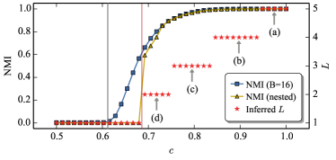
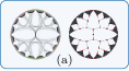
Figure 4: Top: Normalized mutual information (NMI) between the inferred and true partitions for network realizations of the nested PP model described in the text with $B_{1}=2$, $L=5$, ${\left<k\right>}=20$ and $N=10^{4}$, as a function of the assortativity strength $c$, both via the standard stochastic block model with $B=16$, and the nested variant with unspecified parameters. The star symbols ($\star$) show the value of $L$ for the inferred hierarchy. All points are averaged over $20$ independent realizations. The gray vertical line marks the detectability threshold $c^{*}$ when $B$ is predetermined, and the red line when the nested model fails to detect any structure. Bottom: Example hierarchies inferred for the values of $c$ indicated in the top panel. The left image shows the network realization itself, and the right one the hierarchical structure [the planted hierarchy corresponds to the one in (a)].

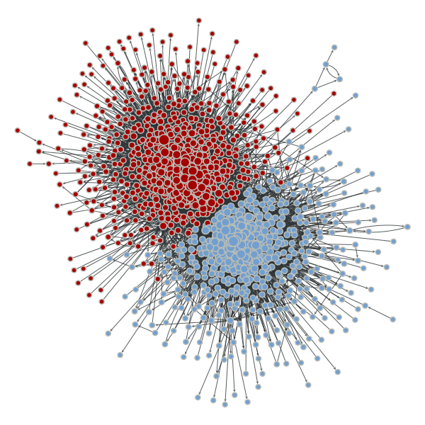
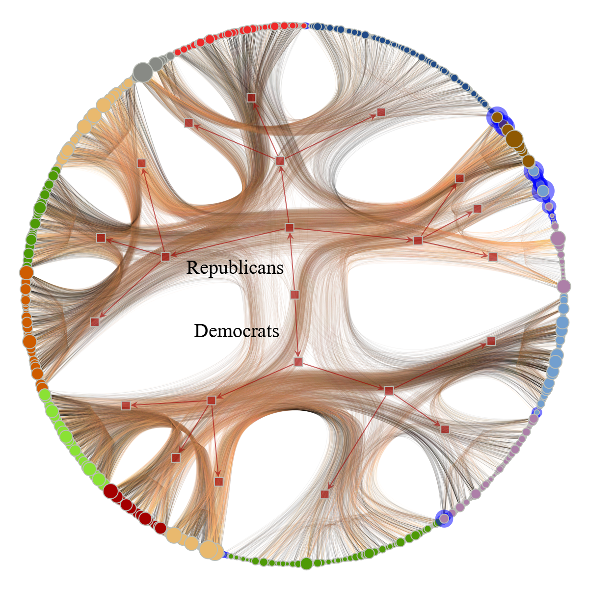
Figure 5: The political blog network of Adamic and Glance Adamic and Glance (2005). Left: Topmost partition of the hierarchy inferred with the nested model. Right: The same network, using a circular layout, with edge bundling following the inferred hierarchy Holten (2006) (indicated also by the square nodes, and the node colors). The size of the nodes corresponds to the total degree, and the edge color indicates its direction (from dark to light). Nodes marked with a blue halo were incorrectly classified at the topmost level, according to the accepted partition in Ref. Adamic and Glance (2005)

In Fig. 4 we show the results of the inference procedure for a generated model with $B_{0}=2$ and $L=5$, $N=10^{4}$ nodes and ${\left<k\right>}=20$. The correct number of blocks is detected up to a given value of $c>c^{*}$, where $c^{*}$ is the detectability threshold. The hierarchy itself matches the nested PP model exactly only for higher values of $c$, and becomes progressively simplified for lower values. Note that for a large fraction of $c$ values the correct lower-level partition is detected with a very high precision, but the hierarchy that is inferred can be simpler than the planted one. In these cases, however, both the inferred hierarchy, as well as the planted model are fully equivalent, i.e. they generate the same networks [this is true for the (a), (b) and (c) regions in Fig. 4, which have $B_{0}=16$]. In other words, the shallower hierarchies that are inferred correspond to identical representations of the same $e_{rs}$ matrix at the lowest level, which require less information to be described, in comparison to the sequence of Kronecker products used in the model specification, and, hence, cannot really be seen as a failure of the inference method, since it simply manages to compress the original model. Before the value of $c$ reaches the detectability threshold, the inference method settles on a fully random $L=1,B=1$ structure, corresponding once again to a parameter region where the block detection is only possible with limited precision and if one knows the correct model size. As predicated by the MDL criterion, the inferred models tend to be as simple as possible, with the hierarchies becoming shallower as one approaches a random graph. The approach is, therefore, conservative, which brings confidence to the blocks and hierarchies that are actually found, since despite the increased resolution capabilities it does not tend to find spurious hierarchies.

In Appendix B we also include a comparison of the method with other algorithms for community detection that are not based on statistical inference.

V Empirical Networks

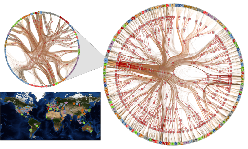
Figure 6: Large-scale structure of the Internet at the autonomous systems level, as obtained by the nested stochastic block model, displaying a prominent core-periphery architecture. The magnification shows the nodes that belong to the “core” top-level branch, containing AS nodes spread all over the globe, as shown in the map inset. See the Supplemental Material for a higher-resolution version of this figure.

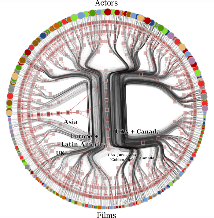
Figure 7: Large-scale structure of the IMDB film-actor network. Each node in this graph represents a lowest-level block in the hierarchy, instead of individual nodes in the graph. The size of the nodes indicates the number of nodes in each group. The hierarchy branch at the top are the actors, and at the bottom are the films. The labels classify each branch according to the most prominent geographical and temporal characteristics found in the database. See the Supplemental Material for a higher-resolution version of this figure.

\begin{overpic}[width=106.23808pt]{scatter-Bdens-E-flat.pdf} \put(24.0,61.0){(a)} \end{overpic}

\begin{overpic}[width=106.23808pt]{scatter-Bdens-E.pdf} \put(24.0,61.0){(b)} \end{overpic}

\begin{overpic}[width=106.23808pt]{scatter-DL-E.pdf} \put(20.0,63.0){(c)} \end{overpic}

\begin{overpic}[width=106.23808pt]{scatter-Q-DL.pdf} \put(22.0,65.0){(d)} \end{overpic}

No.	$N$	$E$	Dir.	No.	$N$	$E$	Dir.	No.	$N$	$E$	Dir.
0	$62$	$159$	No	11	$21,363$	$91,286$	No	22	$255,265$	$2,234,572$	Yes
[2pt] 1	$105$	$441$	No	12	$27,400$	$352,504$	Yes	23	$317,080$	$1,049,866$	No
2	$115$	$613$	No	13	$34,401$	$421,441$	Yes	24	$325,729$	$1,469,679$	Yes
[2pt] 3	$297$	$2,345$	Yes	14	$39,796$	$301,498$	Yes	25	$334,863$	$925,872$	No
4	$903$	$6,760$	No	15	$52,104$	$399,625$	Yes	26	$372,547$	$1,812,312$	No
[2pt] 5	$1,222$	$19,021$	Yes	16	$56,739$	$212,945$	No	27	$449,087$	$4,690,321$	Yes
6	$4,158$	$13,422$	No	17	$75,877$	$508,836$	Yes	28	$654,782$	$7,499,425$	Yes
[2pt] 7	$4,941$	$6,594$	No	18	$82,168$	$870,161$	Yes	29	$855,802$	$5,066,842$	Yes
8	$8,638$	$24,806$	No	19	$105,628$	$2,299,623$	No	30	$1,134,890$	$2,987,624$	No
[2pt] 9	$11,204$	$117,619$	No	20	$196,591$	$950,327$	No	31	$1,637,868$	$15,205,016$	No
10	$17,903$	$196,972$	No	21	$224,832$	$394,400$	Yes	32	$3,764,117$	$16,511,740$	Yes

No.	Network	No.	Network	No.	Network
0	Dolphins Lusseau et al. (2003)	11	arXiv Co-Authors (cond-mat) Leskovec et al. (2007)	22	Web graph of stanford.edu. Leskovec et al. (2008)
[2pt] 1	Political Books	12	arXiv Citations (hep-th) Leskovec et al. (2007); Gehrke et al. (2003)	23	DBLP collaboration Yang and Leskovec (2012)
2	American Football Girvan and Newman (2002); Evans (2012)	13	arXiv Citations (hep-ph) Leskovec et al. (2007); Gehrke et al. (2003)	24	WWW Albert et al. (1999)
[2pt] 3	C. Elegans Neurons Watts and Strogatz (1998)	14	PGP Richters and Peixoto (2011)	25	Amazon product network Yang and Leskovec (2012)
4	Disease Genes Goh et al. (2007)	15	Internet AS (Caida)	26	IMDB film-actor Peixoto (2013a) (bipartite)
[2pt] 5	Political Blogs Adamic and Glance (2005)	16	Brightkite social network Cho et al. (2011)	27	APS citations
6	arXiv Co-Authors (gr-qc) Leskovec et al. (2007)	17	Epinions.com trust network Richardson et al. (2003)	28	Berkeley/Stanford web graph Leskovec et al. (2008)
[2pt] 7	Power Grid Watts and Strogatz (1998)	18	Slashdot Leskovec et al. (2010b)	29	Google web graph Leskovec et al. (2008)
8	arXiv Co-Authors (hep-th) Leskovec et al. (2007)	19	Flickr McAuley and Leskovec (2012)	30	Youtube social network Yang and Leskovec (2012)
[2pt] 9	arXiv Co-Authors (hep-ph) Leskovec et al. (2007)	20	Gowalla social network Cho et al. (2011)	31	Yahoo groups (bipartite)
10	arXiv Co-Authors (astro-ph) Leskovec et al. (2007)	21	EU email Leskovec et al. (2007)	32	US patent citations Leskovec et al. (2005)

Figure 8: (a) The average block size $N/B$ obtained using the nonhierarchical model, as a function of $E$, for the empirical networks listed in the bottom table. The dashed line shows a $\sqrt{E}$ slope. (b) The same as (a) but with the nested model. (c) The description length $\Sigma/E$ for the nested model as a function of $E$. (d) The value of modularity $Q$ as function of $\Sigma/E$, for the nested model.

Here, we present a detailed analysis of some selected empirical networks, as well as a meta-analysis of several networks, spanning different domains and size scales. In all cases, we use the degree-corrected stochastic block model at the lowest hierarchical level, instead of the traditional model, since it almost always provides better results.

Political blogs of the 2004 US election. This is a network compiled by Adamic et al Adamic and Glance (2005) of political blogs during the 2004 presidential election in the USA. The nodes are $N=1,222$ individual blogs, and $E=19,027$ directed edges exist between pairs of blogs, if one blog cites the other. This network is often used as an empirical example of community structure, since it displays a division along political lines, with two clearly distinct groups representing those aligned with the Republican and the Democratic parties. Indeed, if one applies the nested block model to this network, the topmost division in the hierarchy corresponds exactly to this bimodal partition, which closely matches the accepted division (see Fig. 5). This partition is also obtained with the nonhierarchical stochastic block model if one imposes $B=2$ Karrer and Newman (2011). However, the nested version reveals a much more complete picture of the network, where these two partitions possess a detailed internal structure, culminating in $B_{0}=15$ subgroups with quite heterogeneous connection patterns. For instance, one can see that each of the two higher-level groups possesses one or more subgroups composed mainly of peripheral nodes, i.e., blogs that cite other blogs, but are not themselves cited as often. Conversely, both factions possess subgroups which tend to be cited by most other groups, and others which are cited predominantly by specific groups. It is also interesting to note that a large fraction of the connections between the two top-level groups are concentrated between only two specific subgroups, which, therefore, act as bridges between the larger groups.

This example shows that the model is capable of revealing the structure of the network at multiple scales, which reveal simultaneously the existence of the bimodal large-scale division, as well the lower-level subdivisions.

The Autonomous Systems (AS) topology of the Internet. Autonomous Systems (AS) are intermediary building blocks of the Internet topology. They represent organizational units that are used to control the routing of packets in the network. A single AS often corresponds to a network of its own, which is usually owned by a private company, or a government body. The network analyzed here corresponds to the traffic of information between the AS nodes, as measured by the CAIDA project. Each node in the network is an AS, and a directed link exists between two nodes if direct traffic has been observed between the two AS. As of September 2013 the network is composed of $N=52,104$ AS nodes and $E=399,625$ direct connections between them. The application of the nested block model to this network yields the hierarchy seen in Fig. 6, with $B=191$ blocks at the lowest level. The most prominent feature observed is a strong core-periphery structure, where most connections go through a relatively small group of nodes, which act as hubs in the network. The groups both in the core and in the periphery seem strongly correlated to geographical location. However, the nodes of the core groups are not confined to a single geographical location, and are instead spread all over the globe (see inset of Fig. 6, and the Supplemental Material).

The Film-Actor Network. This network is compiled by extracting information available in the Internet Movie Database (IMDB), which contains each cast member and film as distinct nodes, and an undirected edge exists between a film and each of its cast members. If nodes with a single connection are recursively removed, a network of $N=372,447$ and $E=1,812,312$ remains (as of late 2012). As can be seen in Fig. 7, the nested block model fully captures the bipartite nature of the network, and separates movies and actors at the topmost hierarchical level, and proceeds to separate them in geographical, temporal and topical (genre) lines. The observed partition is similar to the one obtained via the nonhierarchical model Peixoto (2013a), but one finds $B=971$ blocks, instead of $B=332$ with the flat version.

Meta-analysis of several empirical networks. We perform an analysis of several empirical networks shown in Fig. 8, which belong to a wide variety of domains, and are distributed across many size scales. We used the nonhierarchical stochastic block model as well as the nested variant. In Fig. 8(a) and (b), we shown the average block sizes $N/B$ for all networks using both models. For the nonhierarchical version, a clear $N/B\sim\sqrt{E}$ trend is observed, which corresponds to the resolution limit present with this method, and other approaches as well. In Fig. 8(b) are shown the results for the nested model, where such a trend can no longer be observed, and the smallest average block sizes no longer seem to depend on the size of the network, which serves as an empirical demonstration of the lack of resolution limit shown previously. The values of the description lengths themselves are also distributed in a seemingly nonorganized manner [see Fig. 8(c)], i.e. no general tendency for larger networks can be observed, other than an increased range of possible values for larger $E$ values. Any difference observed seems to be due to the actual topological organization, rather than intrinsic constraints imposed by the method. We also compute the modularity of the inferred block structures, $Q=\sum_{r}e_{rr}/2E-e_{r}^{2}/(2E)^{2}$, which measures how assortative the topology is. Higher values of $Q$ close to $1$ indicate the existence of densely connected communities. The value of $Q$ is the most common quantity used to detect blocks in networks, and it presumes that such assortative connections are present. In contrast, by fitting a general stochastic block model, no specific pattern is assumed, and the partition found corresponds to the least random model that matches the data. In Fig. 8 we show the values of $Q$ obtained for the analyzed networks. Indeed, some networks are modular, with high values of $Q$. However, one does not observe any strong correlation of the description length and the modularity values. Hence, the most structured networks do not necessarily possess much larger $Q$ values, which indicate that the building blocks of their topological organization are not predominantly assortative communities (this is clear in some of the examples considered previously, such as the Internet AS topology and the IMDB network). However, for many of these networks, it is probably possible to find partitions that lead to much higher $Q$ values. These partitions would, on the other hand, correspond to block model ensembles with a larger entropy than those inferred via maximum likelihood. Therefore, the maximization of $Q$ in these cases would invariably discard topological information present in the network, and provide a much simplified and possibly misleading picture of the large-scale structure of the network. Hence, it seems more appropriate to confine modularity maximization only to cases where the assortative structure is known to be the dominating pattern. However, even in these cases, methods based on statistical inference possess clear advantages, such as the lack of resolution limit, model selection guarantees, and the overall more principled nature of the approach.

VI Discussion

In this paper, we present a principled method to detect hierarchical structures in networks via a nested stochastic block model. This method fully generalizes previous approaches for the detection of hierarchical community structures Clauset et al. (2007, 2008); Rosvall and Bergstrom (2011); Sales-Pardo et al. (2007); Ronhovde and Nussinov (2009); Kovács et al. (2010); Park et al. (2010), since it makes no assumptions either on the actual types of large-scale structures possible (assortative, dissortative, or any arbitrary mixture), or on the hierarchical form, which is not confined to binary trees or dendograms. We show that a major advantage of this approach is that it breaks the so-called resolution limit of approaches, such as modularity optimization and nonhierarchical model inference, where modules smaller than a characteristic size scaling with $\sqrt{N}$ cannot be resolved. With the nested model presented, this characteristic scale is replaced by a much smaller logarithmic dependence, making it, in practice, non-existent for many applications. This increased resolution comes as a result of robust model selection principles, and is integrated with the desirable capacity of differentiating between noise and actual structure, and, therefore, it is not susceptible to the detection of spurious communities. We show that the model is capable of inferring the large-scale features of empirical networks in significant detail, even for very large networks.

This type of approach should, in principle, also be applicable to other model classes, such as those based on overlapping Palla et al. (2005); Airoldi et al. (2008); Lancichinetti et al. (2009); Gopalan and Blei (2013), or link communities Ahn et al. (2010); Ball et al. (2011). We also predict that it should serve as a more refined method of detecting missing information in networks Clauset et al. (2008); Guimerà and Sales-Pardo (2009), as well as for the prediction of the network evolution Liben-Nowell and Kleinberg (2007), determining the more salient topological features Grady et al. (2012); Bianconi et al. (2009), or large-scale functional summaries of the network topology Guimerà and Nunes Amaral (2005).

Appendix A Bayesian model selection (BMS)

In the following we compare Bayesian model selection (BMS) via integrated likelihood with the MDL approach considered in the main text, and we show that they lead to the same criterion if the model constraints are equivalent.

For the purpose of performing BMS, we evoke the most usual definition of the stochastic block model ensemble, where one defines as parameters the probabilities $p_{rs}$ that an edge exists between two nodes belonging to blocks $r$ and $s$. The posterior likelihood of observing a given graph with a block partition $\{b_{i}\}$ and model parameters $\{p_{rs}\}$ is

$$\mathcal{P}(G|\{b_{i}\},\{p_{rs}\},B)=\prod_{rs}p_{rs}^{\frac{e_{rs}}{2}}(1-p_{rs})^{\frac{n_{r}n_{r}-e_{rs}}{2}}.$$ (13)

The inference procedure consists in, as before, maximizing this quantity with respect to the parameters $\{p_{rs}\}$ and the block partition $\{b_{i}\}$. It is easy to see that if one maximizes Eq. 13 with respect to $\{p_{rs}\}$, one recovers $\max_{\{p_{rs}\}}\ln\mathcal{P}(G|\{b_{i}\},\{p_{rs}\},B)=-\mathcal{S}_{t}$, given in Eq. 1, so indeed these models are equivalent. However this does not provide a means for model selection, since models with a larger number of blocks $B$ will invariably posses a larger likelihood. Instead, the Bayesian model selection approach is to consider the joint probability $\mathcal{P}(G,\{b_{i}\},\{p_{rs}\},\{p_{r}\}|B)$ of observing not only the graph, but also the partition $\{b_{i}\}$, the model parameters $\{p_{rs}\}$ as well as the parameters $\{p_{r}\}$ that control the probability of each partition $\{b_{i}\}$ being observed, which is given by

$$\mathcal{P}(\{b_{i}\}|\{p_{r}\},B)=\prod_{r}p_{r}^{n_{r}}.$$ (14)

This invariably leads to the inclusion of prior probabilities of observing the model parameters, $\mathcal{P}(\{p_{rs}\}|B)$ and $\mathcal{P}(\{p_{r}\}|B)$. Now, instead of finding the model parameters that maximize this quantity, we compute the integrated likelihood Biernacki et al. (2000); Daudin et al. (2008); Côme and Latouche (2013),

$$\mathcal{P}(G,\{b_{i}\}|B) =\!\int\!\mathrm{d}p_{rs}\mathrm{d}p_{r}\,\mathcal{P}(G,\{b_{i}\},\{p_{rs}\},\{p_{r}\}|B)$$ (15)

$$\begin{split}=\int\!\mathrm{d}p_{rs}\,\mathcal{P}(G|\{b_{i}\},\{p_{rs}\},B)\mathcal{P}(\{p_{rs}\}|B)\times\\ \int\!\mathrm{d}p_{r}\mathcal{P}(\{b_{i}\}|\{p_{r}\})\mathcal{P}(\{p_{r}\}|B)\end{split}$$ (16)

$$=\mathcal{P}(G|\{b_{i}\},B)\times\mathcal{P}(\{b_{i}\}|B).$$ (17)

By maximizing $\mathcal{P}(G,\{b_{i}\}|B)$, instead of Eq. 13, one should avoid overfitting the data, since the larger models with many parameters are dominated by a majority of choices that fit the data very badly, and, hence, have a smaller contribution in the integral of Eq. 15. Therefore, the maximization of the integrated likelihood also corresponds to an application of Occam’s razor, and one should expect it to deliver results compatible with MDL Grünwald (2007). However, in practice things are more nuanced, since the value of Eq. 15 is heavily dependent on the choice of priors $\mathcal{P}(\{p_{rs}\}|B)$ and $\mathcal{P}(\{p_{r}\}|B)$. For the block partitions themselves, this choice is more straightforward. Since one wants to be agnostic with respect to what block sizes are possible, one should choose a flat prior $\mathcal{P}(\{p_{r}\}|B)=\operatorname{Dirichlet}(\{p_{r}\}|\{\alpha_{r}\})$, with $\alpha_{r}=1$, so that all counts are equally likely. The integral of Eq. 16 is then computed as

$$\ln\mathcal{P}(\{b_{i}\}|B)=-\ln{\textstyle\left(\kern-3.00003pt\left(\genfrac{}{}{0.0pt}{}{B}{N}\right)\kern-3.00003pt\right)}-\ln N!+\sum_{r}\ln n_{r}!,$$ (18)

which is identical to the partition description length of Eq. 7, i.e. $\ln\mathcal{P}(\{b_{i}\}|B)=-\mathcal{L}^{0}_{t}$.

For the block probabilities, on the other hand, the situation is more subtle. A common choice is the flat prior $\mathcal{P}(\{p_{rs}\}|B)=1$ Guimerà and Sales-Pardo (2009); Daudin et al. (2008); Moore et al. (2011); Latouche et al. (2012); Côme and Latouche (2013). This choice is agnostic with respect to what block structures are expected, and it is also practical, since the integral can be evaluated exactly Guimerà and Sales-Pardo (2009); Côme and Latouche (2013),

$$\begin{split}\ln\mathcal{P}(G|\{b_{i}\},B)=-\sum_{r>s}\ln{{n_{r}n_{s}}\choose e_{rs}}+\ln\left(n_{r}n_{s}+1\right)\\ -\sum_{r}\ln{n_{r}^{2}\choose e_{rr}/2}+\ln\left(n_{r}^{2}/2+1\right)\\ \end{split}$$ (19)

$$\simeq-\frac{1}{2}\sum_{rs}n_{r}n_{s}H_{\text{b}}\left(\frac{e_{rs}}{n_{r}n_{s}}\right)-(B+1)\sum_{r}\ln n_{r},$$ (20)

where the approximation in Eq. 20 was made assuming $n_{r}\gg 1$, and $H_{\text{b}}(x)$ is the binary entropy function. However, there is one important issue with this approach. Namely, there is a strong discrepancy between the models generated by the flat prior $\mathcal{P}(\{p_{rs}\}|B)=1$ and most observed empirical networks. Specifically, typical parameters with $p_{rs}=1/2$ sampled by this prior will result in dense networks with average degree ${\left<k\right>}=\sum_{rs}p_{rs}n_{r}n_{s}/N=N/2$. However, most large empirical networks tend to be sparse, with an average degree which is many orders of magnitude smaller than $N$. Hence, as $N$ becomes large, most observed networks will lie in a vanishingly small portion of the parameter space produced by this prior. A better choice would constrain the average degree to something closer to what is observed in the data, but at the same time being otherwise noninformative regarding the block structure. A choice such as $\mathcal{P}(\{p_{rs}\}|B)\propto\delta(\sum_{rs}p_{rs}n_{r}n_{s}-2E)$, where $E$ is the number of edges in the observed network seems appropriate, but the integral in Eq. 16 becomes difficult to solve. Instead, an easier approach is to modify the model sightly, so that the average degree is implicitly constrained. Here, we consider the model variant where the number of edges $E$ is a fixed parameter, and each sampled edge may land between any two nodes belonging to blocks $r$ and $s$ with probability $q_{rs}$, and we have, therefore, $\sum_{r\geq s}q_{rs}=1$. The full posterior likelihood of this model is

$$\mathcal{P}(G|\{b_{i}\},\{q_{rs}\},E,B)=\frac{E!}{\Omega(\{e_{rs}\},\{n_{r}\})}\frac{\prod_{r\geq s}q_{rs}^{m_{rs}}}{\prod_{r\geq s}m_{rs}!},$$ (21)

where $\Omega(\{e_{rs}\},\{n_{r}\})$ is, as before, the number of different graphs with the same block partition and edge counts, and $m_{rs}=e_{rs}$ if $r\neq s$ or $e_{rr}/2$ otherwise. By maximizing Eq. 21 with respect to $\{q_{rs}\}$, one obtains $\max_{\{q_{rs}\}}\ln\mathcal{P}(G|\{b_{i}\},\{q_{rs}\},E,B)\simeq-\ln\Omega(\{e_{rs}\},\{n_{r}\})=-\mathcal{S}_{t}$, as long as $m_{rs}\gg 1$ or $m_{rs}=0$, so it also is equivalent to the previous models in this limit. With this reparametrization, the average degree remains fixed independently of the choice of prior. Therefore, we may finally use a flat prior $\mathcal{P}(\{q_{rs}\}|B)=\operatorname{Dirichlet}(\{q_{rs}\}|\{\alpha_{rs}=1\})$, without the risk of the graphs becoming inadvertently dense, and again the integrated likelihood can be computed exactly,

$$\mathcal{P}(G|\{b_{i}\},B) =\int\!\mathrm{d}q_{rs}\,\mathcal{P}(G|\{b_{i}\},\{q_{rs}\},E,B)\mathcal{P}(\{q_{rs}\}|B)$$ (22)

$$=\left[\Omega(\{e_{rs}\},\{n_{r}\})\times{\textstyle\left(\kern-3.00003pt\left(\genfrac{}{}{0.0pt}{}{\left(\kern-2.10002pt\left(\genfrac{}{}{0.0pt}{}{B}{2}\right)\kern-2.10002pt\right)}{E}\right)\kern-3.00003pt\right)}\right]^{-1}.$$ (23)

By inserting Eq. 23 into Eq. 17, and comparing with equation Eq. 10, we see that $\ln\mathcal{P}(G,\{b_{i}\}|B)=-\Sigma_{L=1}$, and we conclude reassuringly that the MDL approach is fully equivalent to BMS when all model constraints are compatible. In fact, even in the dense case, although not quite the same, the (dense) BMS and MDL penalties are very similar. If one assumes $N\gg B^{2}$, $E\propto N^{2}$, and equal block sizes $n_{r}=N/B$, both penalties become $\sim B(B+1)\ln N+N\ln B$. Therefore, it seems that whatever differences arising from the two approaches stem simply from nuances in the choice of prior probabilities. This comparison also allows us to interpret the nested block model as a hierarchical Bayesian approach, where the priors $\mathcal{P}(\{q_{rs}\}|B)$ are replaced by a nested sequence of priors and hyperpriors, so that their integrated likelihood matches the description length defined previously.

Appendix B Comparison with other community detection methods

In this section we compare results obtained for synthetic networks with popular community detection methods that are not based on statistical inference. Here, we focus not only on the capacity of the method of finding a partition correlated with the planted one, but also on the number of blocks detected. We concentrate on two methods which have been reported to provide good results in synthetic benchmarks Lancichinetti and Fortunato (2009), namely the Louvain method Blondel et al. (2008), based on modularity optimization, and the Infomod method Rosvall and Bergstrom (2008); Rosvall et al. (2009); Rosvall and Bergstrom (2011), based on compression of random walks. We make use of the LFR benchmark Lancichinetti et al. (2008), which corresponds to a specific parametrization of the degree-corrected stochastic block model Karrer and Newman (2011), where both the degree distribution and the block size distribution follow truncated power laws. Here, we employ a parametrization similar to Ref. Lancichinetti and Fortunato (2009), with a degree distribution following a power law with exponent $-2$ and a minimum degree $k_{\text{min}}=5$, and a community size distribution also following a power-law, but with exponent $-1$, and minimum block size of $50$. We also impose the following additional restrictions: The total number of blocks is always fixed at $B=100$, and for every node $i$ belonging to block $r$, its degree $k_{i}$ cannot exceed $\sqrt{n_{r}}$, to avoid intrinsic degree-degree correlations Peixoto (2012). With this parameter choice, the networks generated with $N=2\times 10^{4}$ possess an average degree ${\left<k\right>}\simeq 7.8$. The actual block structure is parametrized as $e_{rs}=(1-c)e_{r}e_{s}/2E+\delta_{rs}ce_{r}$, where $c$ controls the assortativity: For $c=1$ all edges connect nodes of the same block, and for $c=0$ we have a fully random configuration model.

Because the different methods result in quite different numbers of detected blocks, the normalized mutual information (NMI) is not the most appropriate measure of the overlap between partitions in this case. This is due to the fact that, if the number of nodes is kept fixed, the NMI values tend to be larger simply if the number of blocks is increased, even if this larger partition is in no other way more strongly correlated to the true one. Another measure that is less susceptible to this problem is the variation of information (VI) Meilă (2003), defined as

$$\text{VI}(\{x_{i}\},\{y_{i}\})=H(\{x_{i}\})+H(\{y_{i}\})-2I(\{x_{i}\},\{y_{i}\}),$$ (24)

where $H(\{x_{i}\})$ is the entropy of the partition $\{x_{i}\}$ and $I(\{x_{i}\},\{x_{i}\})$ is the (non-normalized) mutual information between $\{x_{i}\}$ and $\{y_{i}\}$. A value of VI equal to zero means that the partitions are identical, whereas any positive value indicates a reduced overlap between them.

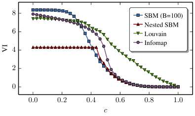
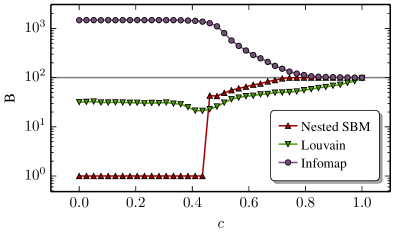
Figure 9: Top: Variation of information (VI) between the planted and obtained partitions as a function of the assortativity parameter $c$, for networks with $N=2\times 10^{4}$, generated as described in the text. The legend indicates results obtained with different methods: Fitting the degree-corrected stochastic block model with a fixed number of blocks $B=100$ (SBM), performing model selection with the nested stochastic block model (Nested SBM), the Louvain modularity maximization method Blondel et al. (2008), and the Infomod method Rosvall and Bergstrom (2008); Rosvall et al. (2009); Rosvall and Bergstrom (2011). Bottom: The obtained number of blocks $B$ as a function of $c$, for the same methods as in the top panel. The gray horizontal line marks the planted $B=100$ value. All results were obtained by averaging over $20$ network realizations.

The VI values between the planted partitions and those obtained with different methods for several network realizations of the above model are shown in Fig. 9, together with the obtained number of blocks. By observing the VI values for the inference method with a fixed number of blocks $B=100$, we conclude that the strict detectability transition (when the value of $B$ is known) lies somewhere slightly above $c\approx 0.2$. However, the model-selection procedure based on the nested stochastic block model presented in the main text discards any structure below the $c\approx 0.4$ range, and decides on a fully random $B=1$ structure. Above this value, the inferred value of $B$ increases from $B=1$ until agreeing with the planted value for sufficiently large $c$ values. As can also be seen in Fig. 9, the Louvain method exhibits the “worst of both worlds,” i.e., it fails to find the correct partition for all values except $c=1$, finding systematically smaller values of $B$, while at the same time finding spurious partitions below the detectability threshold, even when the network is completely random ($c=0$). The Infomod method, on the other hand, seems to find partitions that are largely compatible with the planted one, at least for the parameter region above $c\approx 0.6$. However, for even larger values of $c$, this method detects a number of blocks that is significantly larger than the planted value, which increases steadily as $c$ decreases. Hence, this method is also incapable of separating structure from noise, and finds spurious partitions far below the detectability threshold. Thus, from the three methods analyzed, the one described in the main text is the only one that combines the following three desirable properties: 1. Optimal inference in the detectable range; 2. Guarantee against overfitting and detection of spurious modules; 3. Fully nonparametric implementation.

The suboptimal behavior of the modularity-based method is simply a combination of the resolution limit Fortunato and Barthélemy (2007) and lack of built-in model selection based on statistical evidence Guimerà et al. (2004). It is not currently known if the Infomod method suffers from problems similar to the resolution limit, but clearly it lacks guarantees against detection of spurious modules. Although it is also based on the principle of parsimony, it tries to compress random walks taking place on the network, instead of the network itself. Apparently, the method cannot distinguish between the actual planted block structure and quenched topological fluctuations — both of which will affect random walks — and gradually transitions between the two properties in order to best describe the network dynamics. (As has been shown in Ref. Lancichinetti and Fortunato (2009), this problem diminishes if the average degree of the network is made sufficiently large, in which case the method finally settles in a $B=1$ partition for fully random graphs.) On the other hand, the method in the main text is based on maximizing the likelihood of the exact same generative process that was used to construct the network, which puts it in clear advantage over the other two (and, in fact, many other methods, including all those analyzed in Refs. Lancichinetti et al. (2008); Lancichinetti and Fortunato (2009)), in addition to including a robust and formally motivated model-selection procedure.

Appendix C Directed and undirected networks

As mentioned in the main text, the model described is easily generalized for directed graphs. For the ensemble entropies, we have for the undirected case Peixoto (2012),

$$\mathcal{S}_{t}=\frac{1}{2}\sum_{rs}n_{r}n_{s}H_{\text{b}}\left(\frac{e_{rs}}{n_{r}n_{s}}\right),$$ (25)

while for the directed case it reads,

$$\mathcal{S}^{d}_{t}=\sum_{rs}n_{r}n_{s}H_{\text{b}}\left(\frac{e_{rs}}{n_{r}n_{s}}\right),$$ (26)

where $H_{\text{b}}(x)=-x\ln x-(1-x)\ln(1-x)$ is the binary entropy function. In both cases, $e_{rs}$ is the number of edges from block $r$ to $s$ (or the number of half-edges for the undirected case when $r=s$), and $n_{r}$ is the number of nodes in block $r$. In the sparse limit, $e_{rs}\ll n_{r}n_{s}$, these expressions may be written approximately as

$$\mathcal{S}_{t} \cong E-\frac{1}{2}\sum_{rs}e_{rs}\ln\left(\frac{e_{rs}}{n_{r}n_{s}}\right),$$ (27)

$$\mathcal{S}^{d}_{t} \cong E-\sum_{rs}e_{rs}\ln\left(\frac{e_{rs}}{n_{r}n_{s}}\right).$$ (28)

For the degree-corrected variant with “hard” degree constraints, we have

$$\mathcal{S}_{c} \cong-E-\sum_{k}N_{k}\ln k!-\frac{1}{2}\sum_{rs}e_{rs}\ln\left(\frac{e_{rs}}{e_{r}e_{s}}\right),$$ (29)

$$\begin{split}\mathcal{S}^{d}_{c}&\cong-E-\sum_{k^{+}}N_{k^{+}}\ln k^{+}!-\sum_{k^{-}}N_{k^{-}}\ln k^{-}!\\ &\qquad-\sum_{rs}e_{rs}\ln\left(\frac{e_{rs}}{e^{+}_{r}e^{-}_{s}}\right),\end{split}$$ (30)

where $e_{r}=\sum_{s}e_{rs}$ is the number of half-edges incident on block $r$, and $e^{+}_{r}=\sum_{s}e_{rs}$ and $e^{-}_{r}=\sum_{s}e_{sr}$ are the number of out- and in-edges adjacent to block $r$, respectively. These expressions are also only valid in the sparse limit, which in this case amounts to the following conditions,

$$e_{rs}\frac{{\left<k^{2}\right>}_{r}-{\left<k\right>}_{r}}{{\left<k\right>}^{2}_{r}}\frac{{\left<k^{2}\right>}_{s}-{\left<k\right>}_{s}}{{\left<k\right>}^{2}_{s}}\ll n_{r}n_{s},$$ (31)

where ${\left<k^{l}\right>}_{r}=\sum_{i\in r}k_{i}^{l}/n_{r}$ [for the directed case we simply replace ${\left<k^{l}\right>}_{r}\to{\left<(k^{+})^{l}\right>}_{r}$ and ${\left<k^{l}\right>}_{s}\to{\left<(k^{-})^{l}\right>}_{s}$ in the equation above]. Unfortunately, there is no closed-form expression for the entropy outside the sparse limit, unlike the traditional variant Peixoto (2012).

For the upper-level multigraphs the entropies are Peixoto (2012),

$$\mathcal{S}_{m} =\sum_{r>s}\ln{\textstyle\left(\kern-3.00003pt\left(\genfrac{}{}{0.0pt}{}{n_{r}n_{s}}{e_{rs}}\right)\kern-3.00003pt\right)}+\sum_{r}\ln{\textstyle\left(\kern-3.00003pt\left(\genfrac{}{}{0.0pt}{}{\left(\kern-2.10002pt\left(\genfrac{}{}{0.0pt}{}{n_{r}}{2}\right)\kern-2.10002pt\right)}{e_{rr}/2}\right)\kern-3.00003pt\right)},$$ (32)

$$\mathcal{S}^{d}_{m} =\sum_{rs}\ln{\textstyle\left(\kern-3.00003pt\left(\genfrac{}{}{0.0pt}{}{n_{r}n_{s}}{e_{rs}}\right)\kern-3.00003pt\right)},$$ (33)

where, as before, $\left(\kern-3.00003pt\left(\genfrac{}{}{0.0pt}{}{n}{m}\right)\kern-3.00003pt\right)={n+m-1\choose m}$ is the number of $m$-combinations with repetitions from a set of size $n$.

For the degree-corrected model, the description length needs to be augmented with the information necessary to describe the degree sequence, analogously to Eq. 9 for the undirected case,

$$\mathcal{L}_{c}=\mathcal{L}_{t}+\sum_{r}n_{r}H(\{p^{r}_{k^{-},k^{+}}\}),$$ (34)

where $\{p^{r}_{k^{-},k^{+}}\}$ is the joint (in,out)-degree distribution of nodes belonging to block $r$.

Note that other generalizations for the directed case are possible Zhu et al. (2014), and it should be straightforward to adapt the nested model for them as well.

See pages 1 of sup_inf.pdf See pages 2 of sup_inf.pdf See pages 3 of sup_inf.pdf

References

- Newman (2011) M. E. J. Newman, “Communities, modules and large-scale structure in networks,” Nat Phys 8, 25–31 (2011).
- Fortunato (2010) Santo Fortunato, “Community detection in graphs,” Physics Reports 486, 75–174 (2010).
- Girvan and Newman (2002) M. Girvan and M. E. J. Newman, “Community structure in social and biological networks,” Proceedings of the National Academy of Sciences 99, 7821 –7826 (2002).
- Ravasz et al. (2002) E. Ravasz, A. L. Somera, D. A. Mongru, Z. N. Oltvai, and A.-L. Barabási, “Hierarchical organization of modularity in metabolic networks,” Science 297, 1551–1555 (2002), PMID: 12202830.
- Fletcher Jr et al. (2013) Robert J. Fletcher Jr, Andre Revell, Brian E. Reichert, Wiley M. Kitchens, Jeremy D. Dixon, and James D. Austin, “Network modularity reveals critical scales for connectivity in ecology and evolution,” Nature Communications 4 (2013), 10.1038/ncomms3572.
- Albert et al. (1999) Réka Albert, Hawoong Jeong, and Albert-László Barabási, “Internet: Diameter of the world-wide web,” Nature 401, 130–131 (1999).
- Yook et al. (2002) Soon-Hyung Yook, Hawoong Jeong, and Albert-László Barabási, “Modeling the internet’s large-scale topology,” Proceedings of the National Academy of Sciences 99, 13382–13386 (2002), PMID: 12368484.
- Zhao et al. (2011) Yunpeng Zhao, Elizaveta Levina, and Ji Zhu, “Community extraction for social networks,” Proceedings of the National Academy of Sciences 108, 7321 –7326 (2011).
- Palla et al. (2005) Gergely Palla, Imre Derényi, Illés Farkas, and Tamás Vicsek, “Uncovering the overlapping community structure of complex networks in nature and society,” Nature 435, 814–818 (2005), PMID: 15944704.
- Newman and Girvan (2004) M. E. J. Newman and M. Girvan, “Finding and evaluating community structure in networks,” Physical Review E 69, 026113 (2004).
- Clauset et al. (2004) Aaron Clauset, M. E. J. Newman, and Cristopher Moore, “Finding community structure in very large networks,” Physical Review E 70, 066111 (2004).
- Blondel et al. (2008) Vincent D. Blondel, Jean-Loup Guillaume, Renaud Lambiotte, and Etienne Lefebvre, “Fast unfolding of communities in large networks,” Journal of Statistical Mechanics: Theory and Experiment 2008, P10008 (2008).
- Guimerà et al. (2004) Roger Guimerà, Marta Sales-Pardo, and Luís A. Nunes Amaral, “Modularity from fluctuations in random graphs and complex networks,” Physical Review E 70, 025101 (2004).
- Fortunato and Barthélemy (2007) Santo Fortunato and Marc Barthélemy, “Resolution limit in community detection,” Proceedings of the National Academy of Sciences 104, 36–41 (2007).
- Lancichinetti and Fortunato (2011) Andrea Lancichinetti and Santo Fortunato, “Limits of modularity maximization in community detection,” Physical Review E 84, 066122 (2011).
- Good et al. (2010) Benjamin H. Good, Yves-Alexandre de Montjoye, and Aaron Clauset, “Performance of modularity maximization in practical contexts,” Physical Review E 81, 046106 (2010).
- Hastings (2006) M. B. Hastings, “Community detection as an inference problem,” Physical Review E 74, 035102 (2006).
- Garlaschelli and Loffredo (2008) Diego Garlaschelli and Maria I. Loffredo, “Maximum likelihood: Extracting unbiased information from complex networks,” Physical Review E 78, 015101 (2008).
- Newman and Leicht (2007) M. E. J. Newman and E. A. Leicht, “Mixture models and exploratory analysis in networks,” Proceedings of the National Academy of Sciences 104, 9564 –9569 (2007).
- Reichardt and White (2007) J. Reichardt and D. R. White, “Role models for complex networks,” The European Physical Journal B 60, 217–224 (2007).
- Hofman and Wiggins (2008) Jake M. Hofman and Chris H. Wiggins, “Bayesian approach to network modularity,” Physical Review Letters 100, 258701 (2008).
- Bickel and Chen (2009) Peter J. Bickel and Aiyou Chen, “A nonparametric view of network models and Newman–Girvan and other modularities,” Proceedings of the National Academy of Sciences 106, 21068–21073 (2009).
- Guimerà and Sales-Pardo (2009) Roger Guimerà and Marta Sales-Pardo, “Missing and spurious interactions and the reconstruction of complex networks,” Proceedings of the National Academy of Sciences 106, 22073 –22078 (2009).
- Karrer and Newman (2011) Brian Karrer and M. E. J. Newman, “Stochastic blockmodels and community structure in networks,” Physical Review E 83, 016107 (2011).
- Ball et al. (2011) Brian Ball, Brian Karrer, and M. E. J. Newman, “Efficient and principled method for detecting communities in networks,” Physical Review E 84, 036103 (2011).
- Reichardt et al. (2011) Jörg Reichardt, Roberto Alamino, and David Saad, “The interplay between microscopic and mesoscopic structures in complex networks,” PLoS ONE 6, e21282 (2011).
- Zhu et al. (2014) Yaojia Zhu, Xiaoran Yan, and Cristopher Moore, “Oriented and degree-generated block models: generating and inferring communities with inhomogeneous degree distributions,” Journal of Complex Networks 2, 1–18 (2014).
- Baskerville et al. (2011) Edward B. Baskerville, Andy P. Dobson, Trevor Bedford, Stefano Allesina, T. Michael Anderson, and Mercedes Pascual, “Spatial guilds in the serengeti food web revealed by a bayesian group model,” PLoS Comput Biol 7, e1002321 (2011).
- Decelle et al. (2011a) Aurelien Decelle, Florent Krzakala, Cristopher Moore, and Lenka Zdeborová, “Inference and phase transitions in the detection of modules in sparse networks,” Physical Review Letters 107, 065701 (2011a).
- Decelle et al. (2011b) Aurelien Decelle, Florent Krzakala, Cristopher Moore, and Lenka Zdeborová, “Asymptotic analysis of the stochastic block model for modular networks and its algorithmic applications,” Physical Review E 84, 066106 (2011b).
- Mossel et al. (2012) Elchanan Mossel, Joe Neeman, and Allan Sly, “Stochastic block models and reconstruction,” arXiv:1202.1499 (2012).
- Peixoto (2013a) Tiago P. Peixoto, “Parsimonious module inference in large networks,” Physical Review Letters 110, 148701 (2013a).
- Holland et al. (1983) Paul W. Holland, Kathryn Blackmond Laskey, and Samuel Leinhardt, “Stochastic blockmodels: First steps,” Social Networks 5, 109–137 (1983).
- Fienberg et al. (1985) Stephen E. Fienberg, Michael M. Meyer, and Stanley S. Wasserman, “Statistical analysis of multiple sociometric relations,” Journal of the American Statistical Association 80, 51–67 (1985).
- Faust and Wasserman (1992) Katherine Faust and Stanley Wasserman, “Blockmodels: Interpretation and evaluation,” Social Networks 14, 5–61 (1992).
- Anderson et al. (1992) Carolyn J. Anderson, Stanley Wasserman, and Katherine Faust, “Building stochastic blockmodels,” Social Networks 14, 137–161 (1992).
- Rosvall and Bergstrom (2007) Martin Rosvall and Carl T. Bergstrom, “An information-theoretic framework for resolving community structure in complex networks,” Proceedings of the National Academy of Sciences 104, 7327–7331 (2007).
- Daudin et al. (2008) J.-J. Daudin, F. Picard, and S. Robin, “A mixture model for random graphs,” Statistics and Computing 18, 173–183 (2008).
- Mariadassou et al. (2010) Mahendra Mariadassou, Stéphane Robin, and Corinne Vacher, “Uncovering latent structure in valued graphs: A variational approach,” The Annals of Applied Statistics 4, 715–742 (2010), mathematical Reviews number (MathSciNet): MR2758646.
- Moore et al. (2011) Cristopher Moore, Xiaoran Yan, Yaojia Zhu, Jean-Baptiste Rouquier, and Terran Lane, “Active learning for node classification in assortative and disassortative networks,” in Proceedings of the 17th ACM SIGKDD international conference on Knowledge discovery and data mining, KDD ’11 (ACM, New York, NY, USA, 2011) p. 841–849.
- Latouche et al. (2012) Pierre Latouche, Etienne Birmele, and Christophe Ambroise, “Variational bayesian inference and complexity control for stochastic block models,” Statistical Modelling 12, 93–115 (2012).
- Côme and Latouche (2013) E. Côme and P. Latouche, Model selection and clustering in stochastic block models with the exact integrated complete data likelihood, arXiv e-print 1303.2962 (2013).
- Clauset et al. (2007) Aaron Clauset, Cristopher Moore, and Mark E. J. Newman, “Structural inference of hierarchies in networks,” in Statistical Network Analysis: Models, Issues, and New Directions, Lecture Notes in Computer Science No. 4503, edited by Edoardo Airoldi, David M. Blei, Stephen E. Fienberg, Anna Goldenberg, Eric P. Xing, and Alice X. Zheng (Springer Berlin Heidelberg, 2007) pp. 1–13.
- Clauset et al. (2008) Aaron Clauset, Cristopher Moore, and M. E. J. Newman, “Hierarchical structure and the prediction of missing links in networks,” Nature 453, 98–101 (2008).
- Rosvall and Bergstrom (2011) Martin Rosvall and Carl T. Bergstrom, “Multilevel compression of random walks on networks reveals hierarchical organization in large integrated systems,” PLoS ONE 6, e18209 (2011).
- Sales-Pardo et al. (2007) Marta Sales-Pardo, Roger Guimerà, André A. Moreira, and Luís A. Nunes Amaral, “Extracting the hierarchical organization of complex systems,” Proceedings of the National Academy of Sciences 104, 15224–15229 (2007), PMID: 17881571.
- Ronhovde and Nussinov (2009) Peter Ronhovde and Zohar Nussinov, “Multiresolution community detection for megascale networks by information-based replica correlations,” Physical Review E 80, 016109 (2009).
- Kovács et al. (2010) István A. Kovács, Robin Palotai, Máté S. Szalay, and Peter Csermely, “Community landscapes: An integrative approach to determine overlapping network module hierarchy, identify key nodes and predict network dynamics,” PLoS ONE 5, e12528 (2010).
- Park et al. (2010) Yongjin Park, Cristopher Moore, and Joel S. Bader, “Dynamic networks from hierarchical bayesian graph clustering,” PLoS ONE 5, e8118 (2010).
- Peixoto (2012) Tiago P. Peixoto, “Entropy of stochastic blockmodel ensembles,” Physical Review E 85, 056122 (2012).
- Leskovec et al. (2010a) Jure Leskovec, Deepayan Chakrabarti, Jon Kleinberg, Christos Faloutsos, and Zoubin Ghahramani, “Kronecker graphs: An approach to modeling networks,” J. Mach. Learn. Res. 11, 985–1042 (2010a).
- Bianconi (2009) Ginestra Bianconi, “Entropy of network ensembles,” Physical Review E 79, 036114 (2009).
- Grünwald (2007) Peter D. Grünwald, The Minimum Description Length Principle (The MIT Press, 2007).
- Rissanen (2010) Jorma Rissanen, Information and Complexity in Statistical Modeling, 1st ed. (Springer, 2010).
- Biernacki et al. (2000) C. Biernacki, G. Celeux, and G. Govaert, “Assessing a mixture model for clustering with the integrated completed likelihood,” IEEE Transactions on Pattern Analysis and Machine Intelligence 22, 719–725 (2000).
- Yan et al. (2012) Xiaoran Yan, Jacob E. Jensen, Florent Krzakala, Cristopher Moore, Cosma Rohilla Shalizi, Lenka Zdeborova, Pan Zhang, and Yaojia Zhu, “Model selection for degree-corrected block models,” arXiv:1207.3994 (2012).
- Schwarz (1978) Gideon Schwarz, “Estimating the dimension of a model,” The Annals of Statistics 6, 461–464 (1978), mathematical Reviews number (MathSciNet): MR468014; Zentralblatt MATH identifier: 0379.62005.
- Akaike (1974) H. Akaike, “A new look at the statistical model identification,” IEEE Transactions on Automatic Control 19, 716–723 (1974).
- Reichardt and Leone (2007) Joerg Reichardt and Michele Leone, “(un)detectable cluster structure in sparse networks,” 0711.1452 (2007).
- Hu et al. (2012) Dandan Hu, Peter Ronhovde, and Zohar Nussinov, “Phase transitions in random potts systems and the community detection problem: spin-glass type and dynamic perspectives,” Philosophical Magazine 92, 406–445 (2012).
- Condon and Karp (2001) Anne Condon and Richard M. Karp, “Algorithms for graph partitioning on the planted partition model,” Random Structures & Algorithms 18, 116–140 (2001).
- Xiang et al. (2012) J. Xiang, X. G. Hu, X. Y. Zhang, J. F. Fan, X. L. Zeng, G. Y. Fu, K. Deng, and K. Hu, “Multi-resolution modularity methods and their limitations in community detection,” The European Physical Journal B 85, 1–10 (2012).
- Peixoto (2014) Tiago P. Peixoto, “Efficient monte carlo and greedy heuristic for the inference of stochastic block models,” Physical Review E 89, 012804 (2014).
- Palla et al. (2010) Gergely Palla, László Lovász, and Tamás Vicsek, “Multifractal network generator,” Proceedings of the National Academy of Sciences 107, 7640 –7645 (2010).
- Peixoto (2013b) Tiago P. Peixoto, “Eigenvalue spectra of modular networks,” Physical Review Letters 111, 098701 (2013b).
- Nadakuditi and Newman (2012) Raj Rao Nadakuditi and M. E. J. Newman, “Graph spectra and the detectability of community structure in networks,” Physical Review Letters 108, 188701 (2012).
- Adamic and Glance (2005) Lada A. Adamic and Natalie Glance, “The political blogosphere and the 2004 U.S. election: divided they blog,” in Proceedings of the 3rd international workshop on Link discovery, LinkKDD ’05 (ACM, New York, NY, USA, 2005) p. 36–43.
- Holten (2006) D. Holten, “Hierarchical edge bundles: Visualization of adjacency relations in hierarchical data,” IEEE Transactions on Visualization and Computer Graphics 12, 741–748 (2006).
- Lusseau et al. (2003) David Lusseau, Karsten Schneider, Oliver J. Boisseau, Patti Haase, Elisabeth Slooten, and Steve M. Dawson, “The bottlenose dolphin community of doubtful sound features a large proportion of long-lasting associations,” Behavioral Ecology and Sociobiology 54, 396–405 (2003).
- Leskovec et al. (2007) Jure Leskovec, Jon Kleinberg, and Christos Faloutsos, “Graph evolution: Densification and shrinking diameters,” ACM Trans. Knowl. Discov. Data 1 (2007), 10.1145/1217299.1217301.
- Leskovec et al. (2008) Jure Leskovec, Kevin J. Lang, Anirban Dasgupta, and Michael W. Mahoney, “Community structure in large networks: Natural cluster sizes and the absence of large well-defined clusters,” arXiv:0810.1355 (2008).
- Gehrke et al. (2003) Johannes Gehrke, Paul Ginsparg, and Jon Kleinberg, “Overview of the 2003 KDD cup,” SIGKDD Explor. Newsl. 5, 149–151 (2003).
- Yang and Leskovec (2012) Jaewon Yang and Jure Leskovec, “Defining and evaluating network communities based on ground-truth,” in Proceedings of the ACM SIGKDD Workshop on Mining Data Semantics, MDS ’12 (ACM, New York, NY, USA, 2012) p. 3:1–3:8.
- Evans (2012) T S Evans, “American college football network files,” FigShare (2012), 10.6084/m9.figshare.93179.
- Watts and Strogatz (1998) D. J. Watts and S. H. Strogatz, “Collective dynamics of ’small-world’ networks,” Nature 393, 409–10 (1998).
- Richters and Peixoto (2011) Oliver Richters and Tiago P. Peixoto, “Trust transitivity in social networks,” PLoS ONE 6, e18384 (2011).
- Goh et al. (2007) K. I. Goh, M. E. Cusick, D. Valle, B. Childs, M. Vidal, and A. L. Barabási, “The human disease network,” Proceedings of the National Academy of Sciences 104, 8685 (2007).
- Cho et al. (2011) Eunjoon Cho, Seth A. Myers, and Jure Leskovec, “Friendship and mobility: user movement in location-based social networks,” in Proceedings of the 17th ACM SIGKDD international conference on Knowledge discovery and data mining, KDD ’11 (ACM, New York, NY, USA, 2011) p. 1082–1090.
- Richardson et al. (2003) Matthew Richardson, Rakesh Agrawal, and Pedro Domingos, “Trust management for the semantic web,” in The Semantic Web - ISWC 2003, Lecture Notes in Computer Science No. 2870, edited by Dieter Fensel, Katia Sycara, and John Mylopoulos (Springer Berlin Heidelberg, 2003) pp. 351–368.
- Leskovec et al. (2010b) Jure Leskovec, Daniel Huttenlocher, and Jon Kleinberg, “Signed networks in social media,” in Proceedings of the SIGCHI Conference on Human Factors in Computing Systems, CHI ’10 (ACM, New York, NY, USA, 2010) p. 1361–1370.
- McAuley and Leskovec (2012) Julian McAuley and Jure Leskovec, “Image labeling on a network: Using social-network metadata for image classification,” in Computer Vision – ECCV 2012, Lecture Notes in Computer Science No. 7575, edited by Andrew Fitzgibbon, Svetlana Lazebnik, Pietro Perona, Yoichi Sato, and Cordelia Schmid (Springer Berlin Heidelberg, 2012) pp. 828–841.
- Leskovec et al. (2005) Jure Leskovec, Jon Kleinberg, and Christos Faloutsos, “Graphs over time: densification laws, shrinking diameters and possible explanations,” in Proceedings of the eleventh ACM SIGKDD international conference on Knowledge discovery in data mining, KDD ’05 (ACM, New York, NY, USA, 2005) p. 177–187.
- Airoldi et al. (2008) Edoardo M. Airoldi, David M. Blei, Stephen E. Fienberg, and Eric P. Xing, “Mixed membership stochastic blockmodels,” J. Mach. Learn. Res. 9, 1981–2014 (2008).
- Lancichinetti et al. (2009) Andrea Lancichinetti, Santo Fortunato, and János Kertész, “Detecting the overlapping and hierarchical community structure in complex networks,” New Journal of Physics 11, 033015 (2009).
- Gopalan and Blei (2013) Prem K. Gopalan and David M. Blei, “Efficient discovery of overlapping communities in massive networks,” Proceedings of the National Academy of Sciences 110, 14534–14539 (2013), PMID: 23950224.
- Ahn et al. (2010) Yong-Yeol Ahn, James P. Bagrow, and Sune Lehmann, “Link communities reveal multiscale complexity in networks,” Nature 466, 761–764 (2010).
- Liben-Nowell and Kleinberg (2007) David Liben-Nowell and Jon Kleinberg, “The link-prediction problem for social networks,” Journal of the American Society for Information Science and Technology 58, 1019–1031 (2007).
- Grady et al. (2012) Daniel Grady, Christian Thiemann, and Dirk Brockmann, “Robust classification of salient links in complex networks,” Nature Communications 3, 864 (2012).
- Bianconi et al. (2009) Ginestra Bianconi, Paolo Pin, and Matteo Marsili, “Assessing the relevance of node features for network structure,” Proceedings of the National Academy of Sciences 106, 11433 –11438 (2009).
- Guimerà and Nunes Amaral (2005) Roger Guimerà and Luís A. Nunes Amaral, “Functional cartography of complex metabolic networks,” Nature 433, 895–900 (2005).
- Lancichinetti and Fortunato (2009) Andrea Lancichinetti and Santo Fortunato, “Community detection algorithms: A comparative analysis,” Physical Review E 80, 056117 (2009).
- Rosvall and Bergstrom (2008) Martin Rosvall and Carl T. Bergstrom, “Maps of random walks on complex networks reveal community structure,” Proceedings of the National Academy of Sciences 105, 1118–1123 (2008), PMID: 18216267.
- Rosvall et al. (2009) M. Rosvall, D. Axelsson, and C. T. Bergstrom, “The map equation,” The European Physical Journal Special Topics 178, 13–23 (2009).
- Lancichinetti et al. (2008) Andrea Lancichinetti, Santo Fortunato, and Filippo Radicchi, “Benchmark graphs for testing community detection algorithms,” Physical Review E 78, 046110 (2008).
- Meilă (2003) Marina Meilă, “Comparing clusterings by the variation of information,” in Learning Theory and Kernel Machines, Lecture Notes in Computer Science No. 2777, edited by Bernhard Schölkopf and Manfred K. Warmuth (Springer Berlin Heidelberg, 2003) pp. 173–187.