Efficient Monte Carlo and greedy heuristic for the inference of stochastic block models

Abstract

We present an efficient algorithm for the inference of stochastic block models in large networks. The algorithm can be used as an optimized Markov chain Monte Carlo (MCMC) method, with a fast mixing time and a much reduced susceptibility to getting trapped in metastable states, or as a greedy agglomerative heuristic, with an almost linear $O(N\ln^{2}N)$ complexity, where $N$ is the number of nodes in the network, independent of the number of blocks being inferred. We show that the heuristic is capable of delivering results which are indistinguishable from the more exact and numerically expensive MCMC method in many artificial and empirical networks, despite being much faster. The method is entirely unbiased towards any specific mixing pattern, and in particular it does not favor assortative community structures.

I Introduction

The use of generative models to infer modular structure in networks has been gaining increased attention in recent years Hastings (2006); Garlaschelli and Loffredo (2008); Newman and Leicht (2007); Reichardt and White (2007); Hofman and Wiggins (2008); Bickel and Chen (2009); Guimerà and Sales-Pardo (2009); Karrer and Newman (2011); Ball et al. (2011); Reichardt et al. (2011); Zhu et al. (2012); Baskerville et al. (2011), due to its more general character, and because it allows the use of more principled methodology when compared to more common methods, such as modularity maximization Newman and Girvan (2004). The most popular generative model being used for this purpose is the so-called stochastic block model Holland et al. (1983); Fienberg et al. (1985); Faust and Wasserman (1992); Anderson et al. (1992), where the nodes in the network are divided into $B$ blocks, and a $B\times B$ matrix specifies the probabilities of edges existing between nodes of each block. This simple model generalizes the notion of “community structure” Fortunato (2010) in that it accommodates not only assortative connections, but also arbitrary mixing patterns, including, for example, bipartite, and core-periphery structures. In this context, the task of detecting modules in networks is converted into a process of statistical inference of the parameters of the generative model given the observed data Hastings (2006); Garlaschelli and Loffredo (2008); Newman and Leicht (2007); Reichardt and White (2007); Hofman and Wiggins (2008); Bickel and Chen (2009); Guimerà and Sales-Pardo (2009); Karrer and Newman (2011); Ball et al. (2011); Reichardt et al. (2011); Zhu et al. (2012); Baskerville et al. (2011), which allows one to make use of the robust framework of statistical analysis. Among the many advantages which this approach brings is the capacity of separating noise from structure, such that no spurious communities are found Peixoto (2013a); Rosvall and Bergstrom (2007); Daudin et al. (2008); Mariadassou et al. (2010); Moore et al. (2011); Latouche et al. (2012); Côme and Latouche (2013), increased resolution in the detection of very small blocks based on refined model selection methods Peixoto (2013b), and the identification of fundamental limits in the detection of modular structure Decelle et al. (2011a, b); Mossel et al. (2012); Reichardt and Leone (2008); Hu et al. (2012). However, one existing drawback in the application of statistical inference is the lack of very efficient algorithms, in particular for networks with a very large number of blocks, with a performance comparable to some popular heuristics available for modularity-based methods Clauset et al. (2004); Blondel et al. (2008). Here we present some efficient techniques of performing statistical inference on large networks, which are partially inspired by the modularity-based heuristics, but where special care is taken not to restrict the procedure to purely assortative block structures, and to control the total number of blocks $B$, such that detailed model selection criteria can be used. Furthermore, the method presented functions either as a greedy heuristic, with a fast $O(N\ln^{2}N)$ algorithmic complexity, or as full-fledged Monte Carlo method, which saturates the detectability range of arbitrary modular structure, at the expense of larger running times.

This paper is divided as follows. In Sec. II the stochastic block model is defined, together with the maximum likelihood inference procedure. Sec. III presents an optimized Markov chain Monte Carlo (MCMC) method which is capable of reaching equilibrium configurations more efficiently than more unsophisticated approaches. In Sec. IV the MCMC techniques are complemented with an agglomerative heuristic which successfully avoids metastable states resulting from starting from random partitions and can be used on its own as an efficient and high-quality inference method. In this session we also compare the heuristic to the full MCMC method, for synthetic networks. In Sec. V we compare both methods with several empirical networks. We finally conclude in Sec. VI with a discussion.

II The Stochastic Block Model

The stochastic block model ensemble Holland et al. (1983); Fienberg et al. (1985); Faust and Wasserman (1992); Anderson et al. (1992) is composed of $N$ nodes, divided into $B$ blocks, with $e_{rs}$ edges between nodes of blocks $r$ and $s$ (or, for convenience of notation, twice that number if $r=s$). For many empirical networks, much better results are obtained if degree variability is included inside each block, as in the so-called degree-corrected block model Karrer and Newman (2011), in which one additionally specifies the degree sequence $\{k_{i}\}$ of the graph as an additional set of parameters.

The detection of modules consists in inferring the most likely model parameters which generated the observed network. One does this by finding the best partition $\{b_{i}\}$ of the nodes, where $b_{i}\in[1,B]$ is the block membership of node $i$, in the observed network $G$, which maximizes the posterior likelihood $\mathcal{P}(G|\{b_{i}\})$. Because each graph with the same edge counts $e_{rs}$ are equally likely, the posterior likelihood is $\mathcal{P}(G|\{b_{i}\})=1/\Omega(\{e_{rs}\},\{n_{r}\})$, where $e_{rs}$ and $n_{r}$ are the edge and node counts associated with the block partition $\{b_{i}\}$, and $\Omega(\{e_{rs}\},\{n_{r}\})$ is the number of different network realizations. Hence, maximizing the likelihood is identical to minimizing the microcanonical entropy Bianconi (2009) $\mathcal{S}(\{e_{rs}\},\{n_{r}\})=\ln\Omega(\{e_{rs}\},\{n_{r}\})$, which can be computed Peixoto (2012) as

$$\mathcal{S}_{t}=\frac{1}{2}\sum_{rs}n_{r}n_{s}H_{\text{b}}\left(\frac{e_{rs}}{n_{r}n_{s}}\right),$$ (1)

for the traditional model and

$$\mathcal{S}_{c}\simeq-E-\sum_{k}N_{k}\ln k!-\frac{1}{2}\sum_{rs}e_{rs}\ln\left(\frac{e_{rs}}{e_{r}e_{s}}\right),$$ (2)

for the degree corrected variant, where $E=\sum_{rs}e_{rs}/2$ is the total number of edges, $N_{k}$ is the total number of nodes with degree $k$, $e_{r}=\sum_{s}e_{rs}$ is the number of half-edges incident on block $r$, and $H_{\text{b}}(x)=-x\ln x-(1-x)\ln(1-x)$ is the binary entropy function, and it was assumed that $n_{r}\gg 1$.

These models can be generalized for directed networks, for which corresponding expressions for the entropies are easily obtained Peixoto (2012, 2013a). The methods described in this paper are directly applicable for directed networks as well.

Although minimizing $\mathcal{S}_{t/c}$ allows one to find the most likely partition into $B$ blocks, it cannot be used to find the best value of $B$ itself. This is because the minimum of $\mathcal{S}_{t/c}$ is a strictly decreasing function of $B$, since larger models can always incorporate more details of the observed data, providing a better fit. Indeed, if one minimizes $\mathcal{S}_{t/c}$ over all $B$ values one will always obtain the trivial $B=N$ partition where each node is in its own block, which is not a useful result. The task of identifying the best value of $B$ in a principled fashion is known as model selection, which attempts to separate actual structure from noise and avoid overfitting. In the current context this can be done in a variety of ways, such as using the minimum description length (MDL) criterion Rosvall and Bergstrom (2007); Peixoto (2013a) or performing Bayesian model selection (BMS)  Daudin et al. (2008); Guimerà and Sales-Pardo (2009); Mariadassou et al. (2010); Moore et al. (2011); Latouche et al. (2012); Côme and Latouche (2013). In Ref. Peixoto (2013b) a high-resolution model selection method is presented, which is based on MDL and a hierarchy of nested stochastic block models describing the network topology at multiple scales and is capable of discriminating blocks with sizes significantly below the so-called “resolution limit” present in other model selection procedures, and other community detection heuristics such as modularity optimization Fortunato and Barthélemy (2007). In Ref. Peixoto (2013b) it is also shown that BMS and MDL deliver identical results if the same model constraints are imposed. However, in order to perform model selection, one first needs to find optimal partitions of the network for given values of $B$, which is the subproblem which we consider in detail in this work. Therefore, in the remainder of this paper we will assume that the value of $B$ is a fixed parameter, unless otherwise stated, but the reader should be aware that this value itself can be determined at a later step via model selection, as described e.g. in Refs. Peixoto (2013a, b).

Given a value of $B$, directly obtaining the partition $\{b_{i}\}$ which minimizes $\mathcal{S}_{t/c}$ is in general not tractable, since it requires testing all possible partitions, which is only feasible for very small networks. Instead one must rely on approximate, or stochastic procedures which are guaranteed to sample partitions with a probability given as a function of $\mathcal{S}_{t/c}$, as described in the following section.

III Markov Chain Monte Carlo

The MCMC approach consists in modifying the block membership of each node in a random fashion and accepting or rejecting each move with a probability given as a function of the entropy difference $\Delta S_{t/c}$. If the acceptance probabilities are chosen appropriately and the process is ergodic, i.e., all possible network partitions are accessible, and detailed balance is preserved, i.e., the moves are reversible, after a sufficiently long equilibration time, each observed partition must occur with the desired probability proportional to $\mathcal{P}(G|\{b_{i}\})=e^{-S_{t/c}}$. In this sense, this process is exact, since it is guaranteed to eventually produce the partitions with the desired probabilities, after a sufficient long equilibration (or mixing) time. In practice, the situation is more nuanced, since equilibration times may be very long, and one may not able to sample from a good approximation of the desired distribution, and different ways of implementing the Markov chain leads to different mixing times. The simplest approach one can take is to attempt to move each vertex into one of the $B$ blocks with equal probability. This easily satisfies the requirements of ergodicity and detailed balance, but can be very inefficient. This is particularly so in the case where the value of $B$ is large, and the block structure of the network is well defined, such that the vertex will belong to very few of the $B$ blocks with a non-vanishing probability, which means that most random moves will simply be rejected. A better approach has been proposed in Ref. Peixoto (2013a), which we present here in a slightly generalized fashion, and consists in attempting to move a vertex from block $r$ to $s$ with a probability given by

$$p(r\to s|t)=\frac{e_{ts}+\epsilon}{e_{t}+\epsilon B},$$ (3)

where $t$ is the block label of a randomly chosen neighbor, and $\epsilon>0$ is a free parameter (note that by making $\epsilon\to\infty$ we recover the fully random moves described above). Eq. 3 means that we attempt to guess the block membership of a given node by inspecting the block membership of its neighbors and by using the currently inferred model parameters to choose the most likely blocks to which the original node belongs (see Fig. 1). It should be observed that this move imposes no inherent bias; in particular, it does not attempt to find assortative structures in preference to any other, since it depends fully on the matrix $e_{rs}$ currently inferred. For any choice of $\epsilon>0$, this move proposal fulfills the ergodicity condition, but not detailed balance. However, this can be enforced in the usual Metropolis-Hastings fashion Metropolis et al. (1953); Hastings (1970) by accepting each move with a probability $a$ given by

$$a=\min\left\{e^{-\beta\Delta\mathcal{S}_{t/c}}\frac{\sum_{t}p_{t}^{i}p(s\to r|t)}{\sum_{t}p^{i}_{t}p(r\to s|t)},1\right\},$$ (4)

where $p^{i}_{t}$ is the fraction of neighbors of node $i$ which belong to block $t$, and $p(s\to r|t)$ is computed after the proposed $r\to s$ move (i.e., with the new values of $e_{rt}$), whereas $p(r\to s|t)$ is computed before. The parameter $\beta$ in Eq. 4 is an inverse temperature, which can be used to escape local minima or to turn the algorithm into a greedy heuristic, as discussed below.

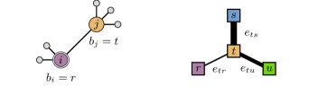
Figure 1: Left: Local neighborhood of node $i$ belonging to block $r$, and a randomly chosen neighbor $j$ belonging to block $t$. Right: Block multigraph, indicating the number of edges between blocks, represented as the edge thickness. In this example, the attempted move $b_{i}\to s$ is made with a larger probability than either $b_{i}\to u$ or $b_{i}\to r$ (no movement), since $e_{ts}>e_{tu}$ and $e_{ts}>e_{tr}$.

The moves with probabilities given by Eq. 3 can be implemented efficiently. We simply write $p(r\to s|t)=(1-R_{t})e_{ts}/e_{t}+R_{t}/B$, with $R_{t}=\epsilon B/(e_{t}+\epsilon B)$. Hence, in order to sample $s$ we proceed as follows: 1. A random neighbor $j$ of the node $i$ being moved is selected, and its block membership $t=b_{j}$ is obtained; 2. The value $s$ is randomly selected from all $B$ choices with equal probability; 3. With probability $R_{t}$ it is accepted; 4. If it is rejected, a randomly chosen edge adjacent to block $t$ is selected, and the block label $s$ is taken from its opposite endpoint. This simple procedure selects the value of $s$ with a probability given by $\sum_{t}p^{i}_{t}p(r\to s|t)$, and requires only a small number of operations, which is independent either on $B$ or the number of neighbors the node $i$ has. The only requirement is that we keep a list of edges which are adjacent to each block, which incurs an additional memory complexity of $O(E)$. To decide whether to accept the move, we need to compute the value of $a$, which can be done in $O(k_{i})$ time, which is the same number of operations which is required to compute $\Delta S_{t/c}$ . Therefore, an entire MCMC sweep of all nodes in the network requires $O(E)$ operations, independent of $B$.

To test the behavior of this approach, we examine a simple example known as the Planted Partition (PP) model Condon and Karp (2001). It corresponds to an assortative block structure given by $e_{rs}=2E[\delta_{rs}c/B+(1-\delta_{rs})(1-c)/B(B-1)]$, $n_{r}=N/B$, and $c\in[0,1]$ is a free parameter which controls the assortativity strength. In this example, the algorithm above leads to much faster mixing times, as can be seen in Fig. 2(left), which shows the autocorrelation function

$$R(\tau)=\frac{\sum_{t=1}^{T-\tau}\left(\mathcal{S}_{t/c}(t)-{\left<\mathcal{S}_{t/c}\right>}\right)\left(\mathcal{S}_{t/c}(t+\tau)-{\left<\mathcal{S}_{t/c}\right>}\right)}{{(T-\tau)\sigma_{\mathcal{S}_{t/c}}^{2}}},$$ (5)

where $\mathcal{S}_{t/c}(t)$ is the entropy value after $t$ MCMC sweeps, and $T$ is the total number of sweeps, computed after a sufficiently long transient has been discarded. For the particular choice of parameters chosen for Fig. 2, the autocorrelation time is of the order of $10$ sweeps with the optimized moves, and of the order of $100$ sweeps with the fully random variant. Despite the difference in the mixing time, both methods sample from the same distribution, as shown in Fig. 2(right).

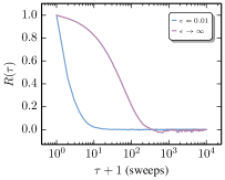
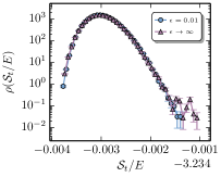
Figure 2: Left: Autocorrelation function $R(\tau)$, for a PP model with $c=0.8$ and $B=100$, for a network of size $N=10^{4}$ and ${\left<k\right>}=10$, and two values of the parameter $\epsilon$, where for $\epsilon\to\infty$ we have fully random moves. The curves were averaged for $100$ independent network realizations. Right: PDF of the values of $\mathcal{S}_{t}/E$ obtained for $T=2\times 10^{4}$ consecutive sweeps for $100$ independent network realizations, for different $\epsilon$ values, showing the same distribution.

The improvement for smaller $\epsilon$ values is more prominent as the block structure becomes more well-defined, as can be seen in Fig. 3, which shows the autocorrelation time $\tau^{*}$, defined here as

$$\tau^{*}=\sum_{\tau=0}^{T^{\prime}}R(\tau),$$ (6)

where $T^{\prime}$ is the largest value of $\tau$ for which $R(\tau)\geq 0$. In Fig. 3(left) are shown the values of $\tau^{*}$ depending on $c$, from which one can see that the relative improvement on the mixing time can be up to two orders of magnitude, for the chosen value of $B=100$. As the value of $c$ approaches the detectability threshold (see below), the autocorrelation time diverges, as is typical of second-order phase transitions, and the relative advantage of the optimized moves diminishes. However, for most of the parameter range where the blocks are detectable, the mixing time with the optimized moves seems independent on the actual number of blocks, as shown in Fig. 3, where a fixed block size $N/B=100$ was used, and $B$ was varied. One can see that for the optimized moves the mixing time remains constant, whereas for the fully random moves it increases steadily with $B$.

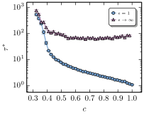
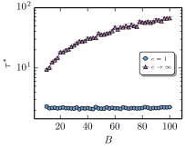
Figure 3: Left: Correlation time $\tau^{*}$ as a function of the model parameter $c$, for different values of $\epsilon$, $N=10^{4}$, ${\left<k\right>}=10$, $B=100$, averaged over $40$ independent network realizations. Right: Correlation time $\tau^{*}$ as a function of the number of blocks $B$, for different values of $\epsilon$, for $N=100\times B$, ${\left<k\right>}=10$, $c=0.8$, averaged over $40$ independent network realizations.

Although the optimized moves above provide a considerable improvement over the fully random alternative whenever the number of blocks $B$ becomes large, there remains an important problem when applying it. Namely, the mixing time can be heavily dependent on how close one starts from the typical partitions which are obtained after equilibration. Since one does not know this, one often starts with a random partition. However, this is very far from the equilibrium states, and if the block structure is sufficiently strong, this can lead to metastable configurations, where the block structure is only partially discovered, as shown in Fig. 4, for a network with $B=3$ . The main problem is that not only does it take a long time to escape such metastable states, but also by observing the values of $S_{t/c}$ alone, one may arrive at the wrong conclusion that the Markov chain has equilibrated. For example, in the simulation shown in Fig. 4, it took many hundreds of sweeps for the final drop in $\mathcal{S}_{t}$ to occur, and before this, the time series is difficult to distinguish from an equilibrated chain. This problem is exacerbated if the average block size $N/B$ increases, which can be frustrating since one would like to consider these scenarios to be easier than for smaller block sizes. In order to avoid this problem, we propose the agglomerative heuristic described in the next session, which can be used as a privileged starting point for the Markov chain, or as an approximate inference tool on its own.

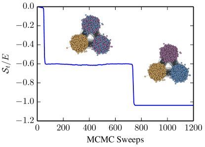
Figure 4: Evolution of the MCMC for a network sampled from the PP model with $N=10^{4}$, ${\left<k\right>}=10$, $B=3$ and $c=0.99$, starting from a fully random partition of the nodes. The networks show a representative snapshot of the state of the system before and after the last drop in $\mathcal{S}_{t}$.

IV Agglomerative Heuristic

In order to avoid the metastable states described previously, we explore the fact that they are more likely to occur if the block sizes are large, since otherwise the quenched topological fluctuations present in the network will offer a smaller free-energy barrier which needs to be overcome. Therefore, a more promising approach is to attempt to find the best configuration for some $B^{\prime}>B$, and then use that configuration to obtain a better estimate for one with $B$ blocks . This can be done by merging blocks together progressively, as shown in Fig. 5. We implement this by constructing a block (multi)graph, where the blocks themselves are the nodes (weighted by the block sizes) and the edge counts $e_{rs}$ are the edge multiplicities between each block node. In this representation, a block merge is simply a block membership move of a block node, where initially each node is in its own block. The choice of moves is done with same probability as before, i.e. via Eq. 3. In order to select the best merges, we attempt $n_{m}$ moves for each block node, and collectively rank the best moves for all nodes according to $\Delta S_{t/c}$. From this global ranking, we select the best $B^{\prime}-B$ merges to obtain the desired partition into $B$ blocks. However if the value of $N/B^{\prime}$ itself is too large, we face again the same problem as before. Therefore we proceed iteratively by starting with $B_{1}=N$, and selecting $B_{i+1}=B_{i}/\sigma$, until we reach the desired $B$ value, where $\sigma>1$ controls how greedily the merges are performed. To diminish the effect of bad merges done in the earlier steps, we also allow individual node moves between each merge step, by applying the MCMC steps above to the original network, with $\beta\to\infty$. The complexity of each agglomerative step is $O[n_{m}E+N\ln(B_{i}-B_{i-1})+\tau E]$, which incorporates the search for the merge candidates, the ranking of the $B_{i}-B_{i-1}$ best merges, and the movement of the individual nodes, where $\tau$ is the necessary amount of sweeps to reach a local minimum. Since we have in total $\ln(N/B)/\ln\sigma$ merge steps, with the slowest one being the first with $B_{1}=N$, we have an overall complexity of $O\{[(n_{m}+\tau)E+N\ln N]\times\ln N/\ln\sigma\}\sim O(N\ln^{2}N)$, if we assume that $B\ll N$  and that the graph is sparse with $E\sim O(N)$.

Despite its greedy nature, we found that this approach is capable of almost always avoiding the metastable configurations described previously, and often comes very close or even exactly to the planted partition (see Fig. 6).

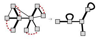
Figure 5: Representation of the block merges used in the agglomerative heuristic. Each square node is a block in the original graph, and the merges (represented as red dashed lines) correspond simply to block membership moves.

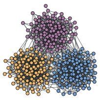
Figure 6: Left: An example of a typical partition obtained by starting with a random $B=3$ configuration and applying only greedy moves, until no further improvement is possible, for a PP network with $N=300$, ${\left<k\right>}=10$, and $c=0.9$. Right: A typical outcome for the same network, with the greedy agglomerative algorithm described in the text.

The parameters $n_{m}$, $\sigma$ and $\epsilon$ allow one to choose an appropriate trade-off between quality and speed. The best results are obtained for large $n_{m}$ and small $\sigma$, however these need not to be chosen fully independently. We found that setting $n_{m}$ to a “reasonable” value such as $10$ or $100$, and selecting $\sigma$ to be $2$, $1.1$ or $1.01$ allows one to probe the full quality range of the algorithm (see below). The choice of the value $\epsilon$ is interesting, since making $\epsilon=0$ allows one to preserve certain graph invariants throughout the whole procedure. Since at the first merging step when $B_{i}=N$ the $e_{rs}$ matrix is simply the adjacency matrix, the membership moves with $\epsilon=0$ cannot merge nodes which belong to different components, or to different partitions in bipartite networks. It is easy to see that this property is preserved for later merging steps as well, so they are fully reflected in the final block structure. We find that very often this is a desired property, and leads to better block partitions. In situations where it is not desired, it can be disabled by setting $\epsilon>0$.

The algorithm above can be turned into a more robust MCMC method by making $\beta=1$ in the intermediary phase between each merge step, and waiting sufficiently long for the Markov chain to equilibrate. This is a slower, but more exact counterpart to the greedy heuristic variant, which is less susceptible to getting trapped in the metastable states discussed previously. If one wishes to find the minimum of $\mathcal{S}_{t/c}$, one can make $\beta\to\infty$ after the chain has equilibrated, either abruptly (as we do in the results presented in this paper), or slowly via simulated annealing Kirkpatrick et al. (1983).

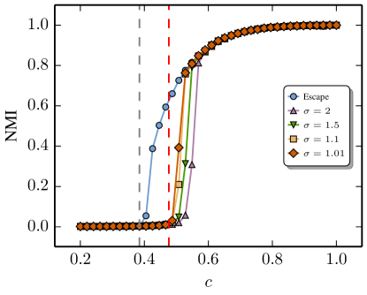
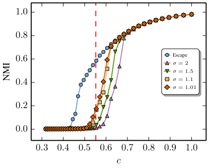
Figure 7: Normalized mutual information (NMI) (see footnote 6) between the planted and the inferred partitions for (top) the PP model and (bottom) the circular multipartite model described in the text, as a function of the modular strength $c$, for $N=10^{4}$ and $B=10$. The “Escape” curves correspond to MCMC equilibrations starting from the planted partition, and the remaining curves to the greedy agglomerative heuristic with ratio $\sigma$ shown in the legend, and $n_{m}=10$. All curves are averaged over $20$ independent network realizations. The grey vertical dashed line corresponds to the detectability threshold $c^{*}$ for the PP model, and the red dashed line to the MDL model selection threshold of Eq. 7.

We can assess the quality of the heuristic method by comparing with known bounds on the detectability of the PP model. If we have that $N/B\gg 1$, it can be shown that for ${\left<k\right>}<[(B-1)/(cB-1)]^{2}$ Decelle et al. (2011a, b); Mossel et al. (2012), it is not possible to detect the planted partition with any method. To emphasize the applicability of the method for dissortative (or arbitrary) topologies, we also analyze a circular multipartite block model, with $e_{rs}=2E\left[\left(\delta_{r,s-1}+\delta_{r,s+1}\right)c/2B+(1-c)/B^{2}\right]$, where $c$ controls the strength of the modular structure, and periodic boundaries are assumed. In both cases we compare the agglomerative heuristic with MCMC results starting from the true partition, which represents the best possible case. As can be seen in Fig. 7, the results from the optimal MCMC and the heuristic are identical for up to some values of $c$ which are larger than the actual detectability threshold. Thus the greedy method falls short of saturating the detectable parameter region, but behaves badly only for a relatively small range of $c$, below which it becomes much harder (but not impossible) to distinguish the observed network from a random graph. To give a more precise idea of the extent to which the graphs in this region deviate from a random topology, we compare with a model selection threshold based on the minimum description length (MDL) principle Peixoto (2013a),

$${\left<k\right>}>\frac{2\ln B}{I_{t/c}},$$ (7)

with $I_{t/c}=(S^{r}_{t/c}-S_{t/c})/E$, where $S_{t/c}^{r}$ is the entropy for a fully random graph, with $e_{rs}=2En_{r}n_{s}/N^{2}$ (or $e_{rs}=e_{r}e_{s}/2E$ for the degree-corrected case), and $E\gg B^{2}$ was assumed. This criterion is useful when we do not know the correct value of $B$, and hence cannot rely on minimizing $S_{t/c}$ alone, since it would always result in a $B=N$ partition. If this condition is not fulfilled, the inferred partition (even if exact) is discarded in favor of a fully random graph, since the model parameters in this case cannot be used to provide a more compact description of the network. From Fig. 7 we see that this threshold lies very close to the region where the agglomerative algorithm is incapable of discovering the optimal partition. Hence, in situations where model selection needs to be performed, any significant improvement to the quality of the algorithm would be ultimately discarded, at least in these specific examples. In other situations, where an increased precision close to the detectability transition is desired, the heuristic should be used only as a component of the full-fledged MCMC procedure with $\beta=1$, as described above, which should be able to eventually reach the optimal configurations, but requires longer running times.

V Performance on empirical networks

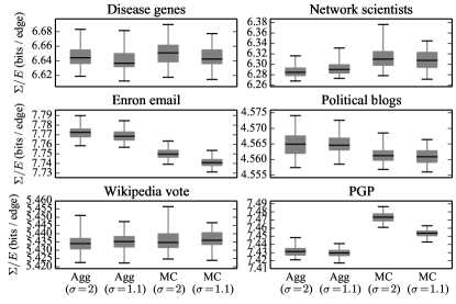
Figure 8: Description length $\Sigma$ for different empirical networks, collected for $100$ independent runs of the MCMC algorithm (MC) and the agglomerative heuristic (Agg), for different agglomeration ratios $\sigma$.

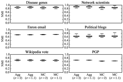
Figure 9: Normalized mutual information (NMI) between the best overall partition and each one collected for $100$ independent runs of the MCMC algorithm (MC) and the agglomerative heuristic (Agg), for different agglomeration ratios $\sigma$.

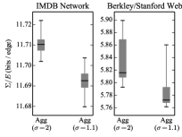
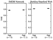
Figure 10: Description length $\Sigma$ for different empirical networks, as well the Normalized mutual information (NMI) between the best overall partition and each one, collected for $100$ independent runs of the agglomerative heuristic, for different agglomeration ratios $\sigma$.

We have analyzed a few empirical networks to assess the behaivor of the algorithm in realistic situations. We have chosen the following networks: The largest component of coauthorships in network science Newman (2006) ($N=379$, $E=914$, undirected), the human disease gene network Goh et al. (2007) ($N=903$, $E=6,760$, undirected), the political blog network Adamic and Glance (2005) ($N=1,222$, $E=19,021$, directed), the Wikipedia vote network Leskovec et al. (2010) ($N=8,298$, $E=103,689$, directed), the Enron email network Klimt and Yang (2004); Leskovec et al. (2008) ($N=36,692,E=367,662$, undirected), the largest strong component of the PGP network Richters and Peixoto (2011) ($N=39,796$, $E=301,498$, directed), the IMDB film-actor network Peixoto (2013a) ($N=372,547$, $E=1,812,312$, undirected), and the Berkeley/Stanford web graph Leskovec et al. (2008) ($N=654,782$, $E=7,499,425$, directed). In all cases we used the degree-corrected model. Since for these networks the most appropriate value of $B$ is unknown, we performed model selection using the MDL criterion as described in Ref. Peixoto (2013a), where we find the partition which minimizes the description length $\Sigma=\mathcal{L}_{t/c}+\mathcal{S}_{t/c}$, where $\mathcal{L}_{t/c}$ is the amount of information necessary to describe the model parameters, which increases with $B$ . For the networks with moderate size we were capable of comparing the results with the agglomerative heuristic to those of the more time consuming MCMC method. Figs. 8 and 10 shown the values of $\Sigma$ after several runs of each algorithm. It can be observed that the results obtained with both methods seem largely indistinguishable for some networks (human diseases, network scientists, and Wikipedia votes), whereas the MCMC algorithm leads to better results for others (Enron email, political blogs), and interestingly to worse results for the PGP network. The better results for MCMC are expected, but the worse result for the PGP network is not. We can explain this by pointing out that for that network the average value of $\mathcal{S}_{c}$ obtained with MCMC for $\beta=1$ noticeably differs from the minimum possible value. Since we used an abrupt cooling to $\beta\to\infty$, the MCMC is more likely to get trapped in a local minimum than the agglomerative heuristic, which is never allowed to heat up to the $\beta=1$ configurations. MCMC would probably match, or even improve the heuristic results if, e.g. simulated annealing would be used to reach the $\beta\to\infty$ region. However, this serves as an example of at least one scenario where the agglomerative heuristic can lead to even better results, despite being much faster than MCMC.

Perhaps a more meaningful comparison among the different results is to determine how the obtained partitions differ from each other. This is shown in Figs. 9 and 10, where the normalized mutual information (NMI)  between the best partition across all runs of all algorithms and every other partition found is compared for the two algorithms. Despite leading to different $\Sigma$ values, the typical partitions found for each algorithm seem equally far from the (approximated) global maximum, so the difference in $\Sigma$ can be attributed to minor differences in the partitions. From this we can conclude the agglomerative heuristic delivers results comparable to MCMC for many empirical networks, while being significantly faster.

Note that the NMI values in Fig. 9 are overall reasonably high, indicating that the partitions are much more similar than different, however they are almost never $1$, or very close to it, except for the smallest networks. This seems to point to a certain degree of degeneracy of optimal partitions, similar to those reported in Ref. Good et al. (2010) for methods based on modularity maximization. A more detailed analysis of this is needed, but we leave it to future work.

VI Conclusion

We have presented an optimized MCMC method  for inferring stochastic block models in large networks, which possesses an improved mixing time due to optimized proposed node membership moves, and an agglomerative procedure which strongly reduces the likelihood of getting trapped in undesired metastable states. By increasing the inverse temperature to $\beta\to\infty$ this method is turned into an agglomerative heuristic, with a fast algorithmic complexity of $O(N\ln^{2}N)$ in sparse networks. We have shown that although the heuristic does not fully saturate the detectability range of the MCMC method, it tends to find indistinguishable partitions for a very large range of parameters of the generative model, as well as for many empirical networks. The method also allows for detailed control of the number of blocks $B$ being inferred, which makes it suitable to be used in conjunction with model selection techniques Peixoto (2013a); Rosvall and Bergstrom (2007); Daudin et al. (2008); Mariadassou et al. (2010); Moore et al. (2011); Latouche et al. (2012); Côme and Latouche (2013); Peixoto (2013b).

The heuristic method is comparable to the agglomerative algorithm of Clauset et al Clauset et al. (2004) (and variants thereof, e.g. Refs. Wakita and Tsurumi (2007); Schuetz and Caflisch (2008a, b)), which has the same overall complexity, but is restricted to finding purely assortative block structures, based on modularity optimization, and is strictly agglomerative, whereas the algorithm presented here permits individual node moves between the blocks at every stage, which allows for the correction of bad merges done in the earliest stages. It can also be compared to the popular method of Blondel et al Blondel et al. (2008), which is not strictly agglomerative, but it is also restricted to assortative structures, and is based on modularity, although it is typically faster than either the method of Clauset et al and the method presented here.

Both the MCMC method and the greedy heuristic compare favorably to many statistical inference methods which depend on obtaining the full marginal probability $\pi_{r}^{i}$ that node $i$ belongs to block $r$ Decelle et al. (2011a, b); Yan et al. (2012). Although this gives more detailed information on the network structure, it does so at the expense of much increased algorithmic complexity. For instance, the belief propagation approach of Refs. Decelle et al. (2011a, b); Yan et al. (2012), although it possesses strong optimal properties, requires $O(NB^{2})$ operations per update sweep, in addition to an $O(EB)$ memory complexity. Since in realistic situations the desired value of $B$ is likely to scale with some power of $N$, this approach quickly becomes impractical and hinders its application to very large networks, in contrast to the log-linear complexity in $N$ (independent of $B$) with the method proposed in this paper.

References

- Hastings (2006) M. B. Hastings, Physical Review E 74, 035102 (2006).
- Garlaschelli and Loffredo (2008) D. Garlaschelli and M. I. Loffredo, Physical Review E 78, 015101 (2008).
- Newman and Leicht (2007) M. E. J. Newman and E. A. Leicht, Proceedings of the National Academy of Sciences 104, 9564 (2007).
- Reichardt and White (2007) J. Reichardt and D. R. White, The European Physical Journal B 60, 217 (2007).
- Hofman and Wiggins (2008) J. M. Hofman and C. H. Wiggins, Physical Review Letters 100, 258701 (2008).
- Bickel and Chen (2009) P. J. Bickel and A. Chen, Proceedings of the National Academy of Sciences 106, 21068 (2009).
- Guimerà and Sales-Pardo (2009) R. Guimerà and M. Sales-Pardo, Proceedings of the National Academy of Sciences 106, 22073 (2009).
- Karrer and Newman (2011) B. Karrer and M. E. J. Newman, Physical Review E 83, 016107 (2011).
- Ball et al. (2011) B. Ball, B. Karrer, and M. E. J. Newman, Physical Review E 84, 036103 (2011).
- Reichardt et al. (2011) J. Reichardt, R. Alamino, and D. Saad, PLoS ONE 6, e21282 (2011).
- Zhu et al. (2012) Y. Zhu, X. Yan, and C. Moore, arXiv:1205.7009 (2012).
- Baskerville et al. (2011) E. B. Baskerville, A. P. Dobson, T. Bedford, S. Allesina, T. M. Anderson, and M. Pascual, PLoS Comput Biol 7, e1002321 (2011).
- Newman and Girvan (2004) M. E. J. Newman and M. Girvan, Physical Review E 69, 026113 (2004).
- Holland et al. (1983) P. W. Holland, K. B. Laskey, and S. Leinhardt, Social Networks 5, 109 (1983).
- Fienberg et al. (1985) S. E. Fienberg, M. M. Meyer, and S. S. Wasserman, Journal of the American Statistical Association 80, 51 (1985).
- Faust and Wasserman (1992) K. Faust and S. Wasserman, Social Networks 14, 5 (1992).
- Anderson et al. (1992) C. J. Anderson, S. Wasserman, and K. Faust, Social Networks 14, 137 (1992).
- Fortunato (2010) S. Fortunato, Physics Reports 486, 75 (2010).
- Peixoto (2013a) T. P. Peixoto, Physical Review Letters 110, 148701 (2013a).
- Rosvall and Bergstrom (2007) M. Rosvall and C. T. Bergstrom, Proceedings of the National Academy of Sciences 104, 7327 (2007).
- Daudin et al. (2008) J.-J. Daudin, F. Picard, and S. Robin, Statistics and Computing 18, 173 (2008).
- Mariadassou et al. (2010) M. Mariadassou, S. Robin, and C. Vacher, The Annals of Applied Statistics 4, 715 (2010), mathematical Reviews number (MathSciNet): MR2758646.
- Moore et al. (2011) C. Moore, X. Yan, Y. Zhu, J.-B. Rouquier, and T. Lane, in Proceedings of the 17th ACM SIGKDD international conference on Knowledge discovery and data mining, KDD ’11 (ACM, New York, NY, USA, 2011) p. 841–849.
- Latouche et al. (2012) P. Latouche, E. Birmele, and C. Ambroise, Statistical Modelling 12, 93–115 (2012).
- Côme and Latouche (2013) E. Côme and P. Latouche, Model selection and clustering in stochastic block models with the exact integrated complete data likelihood, arXiv e-print 1303.2962 (2013).
- Peixoto (2013b) T. P. Peixoto, Hierarchical block structures and high-resolution model selection in large networks, arXiv e-print 1310.4377 (2013).
- Decelle et al. (2011a) A. Decelle, F. Krzakala, C. Moore, and L. Zdeborová, Physical Review Letters 107, 065701 (2011a).
- Decelle et al. (2011b) A. Decelle, F. Krzakala, C. Moore, and L. Zdeborová, Physical Review E 84, 066106 (2011b).
- Mossel et al. (2012) E. Mossel, J. Neeman, and A. Sly, arXiv:1202.1499 (2012).
- Reichardt and Leone (2008) J. Reichardt and M. Leone, Physical Review Letters 101, 078701 (2008).
- Hu et al. (2012) D. Hu, P. Ronhovde, and Z. Nussinov, Philosophical Magazine 92, 406 (2012).
- Clauset et al. (2004) A. Clauset, M. E. J. Newman, and C. Moore, Physical Review E 70, 066111 (2004).
- Blondel et al. (2008) V. D. Blondel, J.-L. Guillaume, R. Lambiotte, and E. Lefebvre, Journal of Statistical Mechanics: Theory and Experiment 2008, P10008 (2008).
- Bianconi (2009) G. Bianconi, Physical Review E 79, 036114 (2009).
- Peixoto (2012) T. P. Peixoto, Physical Review E 85, 056122 (2012).
- Fortunato and Barthélemy (2007) S. Fortunato and M. Barthélemy, Proceedings of the National Academy of Sciences 104, 36 (2007).
- Metropolis et al. (1953) N. Metropolis, A. W. Rosenbluth, M. N. Rosenbluth, A. H. Teller, and E. Teller, The Journal of Chemical Physics 21, 1087 (1953).
- Hastings (1970) W. K. Hastings, Biometrika 57, 97 (1970).
- Condon and Karp (2001) A. Condon and R. M. Karp, Random Structures & Algorithms 18, 116–140 (2001).
- Kirkpatrick et al. (1983) S. Kirkpatrick, C. D. Gelatt Jr, and M. P. Vecchi, Science 220, 671 (1983).
- Newman (2006) M. E. J. Newman, Physical Review E 74, 036104 (2006).
- Goh et al. (2007) K. I. Goh, M. E. Cusick, D. Valle, B. Childs, M. Vidal, and A. L. Barabási, Proceedings of the National Academy of Sciences 104, 8685 (2007).
- Adamic and Glance (2005) L. A. Adamic and N. Glance, in Proceedings of the 3rd international workshop on Link discovery, LinkKDD ’05 (ACM, New York, NY, USA, 2005) p. 36–43.
- Leskovec et al. (2010) J. Leskovec, D. Huttenlocher, and J. Kleinberg, in Proceedings of the SIGCHI Conference on Human Factors in Computing Systems, CHI ’10 (ACM, New York, NY, USA, 2010) p. 1361–1370.
- Klimt and Yang (2004) B. Klimt and Y. Yang, in CEAS (2004).
- Leskovec et al. (2008) J. Leskovec, K. J. Lang, A. Dasgupta, and M. W. Mahoney, arXiv:0810.1355 (2008).
- Richters and Peixoto (2011) O. Richters and T. P. Peixoto, PLoS ONE 6, e18384 (2011).
- Good et al. (2010) B. H. Good, Y.-A. de Montjoye, and A. Clauset, Physical Review E 81, 046106 (2010).
- Wakita and Tsurumi (2007) K. Wakita and T. Tsurumi, in Proceedings of the 16th International Conference on World Wide Web, WWW ’07 (ACM, New York, NY, USA, 2007) p. 1275–1276.
- Schuetz and Caflisch (2008a) P. Schuetz and A. Caflisch, Physical Review E 77, 046112 (2008a).
- Schuetz and Caflisch (2008b) P. Schuetz and A. Caflisch, Physical Review E 78, 026112 (2008b).
- Yan et al. (2012) X. Yan, J. E. Jensen, F. Krzakala, C. Moore, C. R. Shalizi, L. Zdeborova, P. Zhang, and Y. Zhu, arXiv:1207.3994 (2012).