Quantum dot spin cellular automata for realizing a quantum processor

Abstract

We show how single quantum dots, each hosting a singlet-triplet qubit, can be placed in arrays to build a spin quantum cellular automaton. A fast ($\sim 10$ ns) deterministic coherent singlet-triplet filtering, as opposed to current incoherent tunneling/slow-adiabatic based quantum gates (operation time $\sim 300$ ns), can be employed to produce a two-qubit gate through capacitive (electrostatic) couplings that can operate over significant distances. This is the coherent version of the widely discussed charge and nano-magnet cellular automata, and would increase speed, reduce dissipation, and perform quantum computation while interfacing smoothly with its classical counterpart. This combines the best of two worlds – the coherence of spin pairs known from quantum technologies, and the strength and range of electrostatic couplings from the charge-based classical cellular automata. Significantly our system has zero electric dipole moment during the whole operation process, thereby increasing its charge dephasing time.

Keywords: quantum computation, quantum dot, cellular automata, spin qubit

1 Introduction

A coherent version of the widely discussed charge and nano-magnet cellular automata [1, 2, 3] would offer increased speed, reduced dissipation, and would perform quantum computation while interfacing smoothly with its classical counterpart. However, maintaining long time coherence is a challenge [4]. It is appealing to use quantum dot (QD) spins, with coherence times of $\sim 260$ $\mu$s, [5, 6, 7, 8, 9, 10] and in particular singlet-triplet electron pairs, which are largely decoherence free [9, 10, 11]. Here we show how “single” QDs, each hosting a singlet-triplet qubit, can be placed in arrays to build a spin quantum cellular automaton. Our proposal combines the best of two worlds – the coherence of spin pairs known from quantum technologies, and the strength and range of electrostatic couplings from charge-based classical cellular automata. A fast ($\sim 10$ ns) deterministic two-qubit gate is accomplished via non-equilibrium (non-adiabatic) dynamics and capacitive interactions in the course of which no electric dipole moment ever arises, thereby increasing charge coherence significantly.

Many double dot proposals for two-qubit gates already exist, using electrostatic interactions [8, 9, 10, 11, 12]. Their nonzero dipole moment during the gate operations, however, causes rapid charge dephasing [10]. Using more symmetric charge configurations, on the other hand, makes the gate operation slow ($\sim 150$ ns) [11]. If charge tunneling in double QDs eventually becomes incoherent due to the long time scale and strong dephasing, then a set time for the gate operation will disappear, rendering the system indeterministic. In view of the increasing speed of control electronics it is thereby worthwhile to consider non-adiabatic tunnelings that do not create dipole moments. Our proposal can also be realized in a ring of four coupled QDs, which is functionally equivalent to the system we study. This ring structure has already been used for charge-based qubits [13], but the spin dependent dynamics has not yet been explored.

Singlet-triplet qubits in double dots face a fundamental obstacle by seeking to exploit coherent charge tunneling for two-qubit gate operations. Indeed, the very limited and short charge dephasing time ($\sim$ 1 ns) is comparable with the charge tunneling times. For instance the 6 $\mu eV$ tunneling rate in Ref. [10] gives a period of $0.7$ ns for coherent oscillations. According to Ref. [14], the dominant source of dephasing in double dot systems is the interaction between the electric dipole of the two electrons with random electric field fluctuations. In double dot systems the asymmetric charge configuration $(0,2)$ has a large dipole moment $\overrightarrow{\mathbf{p}}\sim e\overrightarrow{\mathbf{d}}$, where $\overrightarrow{\mathbf{d}}$ is the separation between the dots, which gives rise to charge decoherence. Motivated by this, we present a system which benefits from an extra charge orbital that always keeps the charge distribution symmetric with zero dipole moment, resulting in much longer charge dephasing times. One can call this a singlet-triplet qubit, which couples to its environment (and indeed any distant qubits in a scalable network with which the couplings are not sought) through its quadrupole moment, as opposed to the dipole. In addition this extra orbital allows for symmetric charge configurations during gate operations, which enables the simultaneous implementation of identical two-qubit gates between all neighboring pairs in a row, as required for generating cluster states for measurement-based quantum computation. Moreover, our quench dynamics is applicable for degenerate qubit (i.e. singlet-triplet) levels so that no relative phase develops between them during storage (non-operative) periods of the qubit. Both the above features are absent in double dot singlet-triplet qubits, because of their asymmetric charge configurations and the need for an initial singlet-triplet gap for adiabatic operation at non-zero speeds.

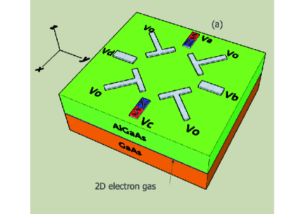
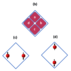
Figure 1: (a) Three dimensional cross-section of the heterostructure junction, showing the gate configuration and location of micro-magnets. As indicated, the $\hat{x}$ and $\hat{y}$ directions lie in the plane of the 2D electron gas, while $\hat{z}$ is perpendicular to it (i.e. the growth direction of the heterostructure). A large negative voltage $V_{0}$ is applied to the “T” gates to impose high potential barriers on the 2D electron gas lying between the AlGaAs and GaAs layers. These barriers define the edges of the square QD. The four remaining finger gates ($V_{a}$, $V_{b}$, $V_{c}$, and $V_{d}$) are used to adjust the local potential in each quadrant of the QD, shown in (b), and thus to control the localization of the two electrons. For simplicity we assume the local potentials are constant within each quadrant. Gates $V_{a}$ and $V_{c}$ are also micro-magnets, used to rotate the spins of the electrons (see Section 5). (b) Labeling of the four quadrants of the square QD. The potential in quadrant $a$ is controlled by gate $V_{a}$, that of quadrant $b$ by $V_{b}$, and so on. Each quadrant has approximate dimensions of $L/2\times L/2$, where $L$ is the side-length of the QD. (c) Charge configuration of $|S_{\leftrightarrow}\rangle$ and $|T_{\leftrightarrow}^{0}\rangle$, in which the electron density is strongly peaked in quadrants $b$ and $d$. (d) Charge configuration of $|S_{\updownarrow}\rangle$ and $|T_{\updownarrow}^{0}\rangle$; in contrast to the previous case the electron density is now localized in quadrants $a$ and $c$. The notation used in the paper of $\updownarrow$ and $\leftrightarrow$ indicate the $x$ and $y$ directions respectively in these diagrams.

2 Two electrons in a square quantum dot

We consider a system of two electrons held in a square semiconductor QD with a hard-wall boundary, approximately realizable by gating a two-dimensional electron gas at a heterojunction interface as shown in Figure 1(a). To describe this system we take as our starting point the effective-mass Hamiltonian for the two interacting electrons:

$$H=-\frac{\hbar^{2}}{{2m^{\ast}}}\left[\nabla_{1}^{2}+\nabla_{2}^{2}\right]+\frac{{e^{2}}}{{4\pi\varepsilon|{\bf{r}}_{1}-{\bf{r}}_{2}|}}+V_{c}({\bf{r}}_{1})+V_{c}({\bf{r}}_{2})+V_{g}({\bf{r}}_{1})+V_{g}({\bf{r}}_{2}),\quad$$ (1)

where $V_{c}(\mathbf{r})$ is the confinement potential and $V_{g}(\mathbf{r})$ is the potential energy due to external gates. The cross-sectional schematic of the heterostructure interface and the gate configuration of the square quantum dot is shown in Figure 1(a). For simplicity we divide the square QD into four quadrants, as shown in Figure 1(b), and apply a constant potential to gates $b$ and $d$ giving an electron potential energy $V_{g}=V$ in quadrants $b$ and $d$, while $V_{g}=0$ when the electrons are in quadrants $a$ and $c$ . When $V$ is positive the electron density is enhanced in quadrants $a$ and $c$ (and depleted in quadrants $b$ and $d$), and vice versa when $V$ is negative.

The time-independent Schrödinger equation for the Hamiltonian (1) may be solved numerically. Since total spin is a good quantum number the eigenstates are singlets and triplets. Furthermore, as the total wave function factors into the product of a spatial part and spin part, we need only solve for the spatial component. Under interchange of electron coordinates this will be symmetric for singlet states, and antisymmetric for triplets. In Figure 2 we show the lowest-lying energy levels for two sizes of QD, $L=400$nm and $L=800$ nm, as a function of the gating potential $V$. Throughout this work we shall use material parameters for GaAs, and as the effective Bohr radius for electrons in this material is $a_{B}\simeq 8.8$nm, these two QD sizes correspond to $L=45a_{B}$ and $L=90a_{B}$ respectively. We see that in both cases the energy level structure is similar for small $V$, consisting of a multiplet of two singlets and triplets, well separated from the next higher states. The formation of this isolated multiplet is a general feature of large QDs for which $L\gg a_{B}$. When this condition is satisfied the Coulomb interaction dominates the kinetic energy, causing the electronic charge density to localize near the corners of the QD [15].

We emphasise that although our model and gating scheme are rather simple, our approach does not require perfect square symmetry, or hard walls, or a perfectly flat background potential. In experiment, for example, gating will produce soft-wall confinement, but this effect, together with deviations from symmetry, and roughness in the confining potential arising from disorder, can be accounted for by renormalizing the tunneling (see Equation (4)) between the two charge configurations. The formation of these low-lying localized states is a rather robust effect.

We will use the states in the lowest multiplet as our qubit space. At $V=0$ the two triplet states are degenerate, and the two singlet states have an energy splitting of $2\Delta_{0}$. To choose an optimum size for the QD we must balance two opposing effects. As we can see from Figure 2, in larger QDs the ground state multiplet in the larger QD is more isolated from higher states than for smaller QDs, which will reduce leakage from the qubit space. The tradeoff from using large QDs, however, is that the energy splitting $\Delta_{0}$ drops rapidly with $L$ [15], making the qubit operation time longer and putting more stringent limits on the operating temperature of the device (see Sec. 10). We therefore use the value of $L=400$nm in our study, which provides a reasonable compromise between these effects.

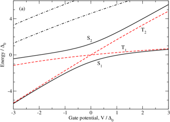
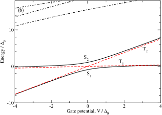
Figure 2: Lowest energy levels of a GaAs QD, obtained by the exact diagonalization of Equation (1). (a) For a QD of size $L=400$nm. Singlet states are shown with solid (black) lines, triplet states with dashed (red) lines. The lowest multiplet consists of the singlet ground state $|S_{1}\rangle$ and excited state $|S_{2}\rangle$, and two $S_{z}=0$ triplet states $|T_{1}\rangle$ and $|T_{2}\rangle$. At $V=0$, the two triplet states are degenerate, and the singlet states have an energy splitting of $2\Delta_{0}$, which we use as the unit of energy. In this case the energy splitting has the value $\Delta_{0}\simeq 20\mu$eV. The black dash-dotted lines indicate the next highest energy levels; near $V=0$ the lowest multiplet of four levels is well-isolated from the rest of the spectrum. (b) As in (a) but for a QD of size $L=800$ nm. The lowest multiplet of states has the same form as in (a), and is even more isolated from the next highest states. The energy splitting reduces as $L$ increases, however, and for this QD size $\Delta_{0}=2.1\mu$eV. This reduction in the energy scale would require lower operating temperatures, and would also give slower qubit operation times.

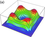
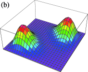
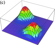
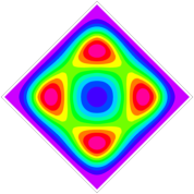
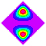
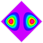
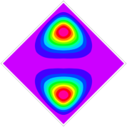
Figure 3: The charge distribution of the two electrons and their contour representations in a square QD of size $L=400$ nm. (a) The charge distribution of $|S_{1}(V=0)\rangle$; the ground state of the two-electron system is a “Wigner molecule” in which the charge density is strongly peaked near the vertices of the QD. (b) The charge distribution of $|S_{\updownarrow}\rangle$. As shown schematically in Fig.1e, the electrons are localized in quadrants $a$ and $c$. (c) The charge distribution of $|S_{\leftrightarrow}\rangle$, shown schematically in Fig.1d. As shown in Equation (2), the ground state charge distribution (a) is a superposition of (b) and (c). (d) The charge distribution of $|S_{1}(V)\rangle$ for $V=3\Delta_{0}$; for large values of the gating potential, the ground state charge distribution strongly resembles the state $|S_{\updownarrow}\rangle$. In the same way $|S_{2}(V)\rangle$ correspondingly approaches $|S_{\leftrightarrow}\rangle$ as $V$ is increased.

For $V=0$ the charge density of the singlet ground state, $|S_{1}\rangle$, for the square QD is shown in Figure 3(a). We see that the charge density is distributed in sharp peaks, located near each of the four corners. Perhaps surprisingly, the charge density for the excited singlet, $|S_{2}\rangle$, has a practically identical charge distribution. This result may be understood by constructing (non-stationary) symmetric and antisymmetric superpositions of the eigenstates as

$$|S_{\updownarrow}\rangle = \frac{|S_{1}(V=0)\rangle-|S_{2}(V=0)\rangle}{\sqrt{2}}$$ (2)

$$|S_{\leftrightarrow}\rangle = \frac{|S_{1}(V=0)\rangle+|S_{2}(V=0)\rangle}{\sqrt{2}}$$ (3)

Note that throughout the paper the states $|S_{\updownarrow}\rangle$ and $|S_{\leftrightarrow}\rangle$ are both defined just for $V=0$ and so unlike $|S_{1}(V)\rangle$ and $|S_{2}(V)\rangle$ have no $V$-dependence. The charge densities of the states $|S_{\updownarrow}\rangle$ and $|S_{\leftrightarrow}\rangle$ are either localized near corners $a$ and $c$ or near corners $b$ and $d$, as shown in Figure 3(b) and Figure 3(c) respectively. These states resemble the states shown schematically in Figure 1(c) and (d) which occur at finite $V$ when gate voltages are applied. The charge density for the state with $V=3\Delta_{0}$ is shown in Figure 3(d) and we see that it indeed looks very similar to the state $|S_{\updownarrow}\rangle$. This similarity may be understood and quantified by expanding the eigenvectors $|S_{1}\rangle$ and $|S_{2}\rangle$ at finite $V$ as superpositions of states $|S_{\updownarrow}\rangle$ and $|S_{\leftrightarrow}\rangle$, defined for $V=0$. For a complete set of states at $V=0$ this expansion is of course exact, but since the lowest two singlets are well separated from higher excited states, we can expect truncation of the basis set to the 2D space of the lowest singlets to be a good approximation, provided $V$ is not too large. Within this 2D subspace the system may be described by the effective Hamiltonian:

$$H_{S}=E_{S_{\updownarrow}}(V)|S_{\updownarrow}\rangle\langle S_{\updownarrow}|+E_{S_{\leftrightarrow}}(V)|S_{\leftrightarrow}\rangle\langle S_{\leftrightarrow}|+\Delta(|S_{\updownarrow}\rangle\langle S_{\leftrightarrow}|+|S_{\leftrightarrow}\rangle\langle S_{\updownarrow}|).$$ (4)

in which

$$E_{S_{\updownarrow}}(V) = \langle S_{\updownarrow}|H|S_{\updownarrow}\rangle=E_{0S}+2Vp^{bd}_{S_{\updownarrow}}$$ (5)

$$E_{S_{\leftrightarrow}}(V) = \langle S_{\leftrightarrow}|H|S_{\leftrightarrow}\rangle=E_{0S}+2Vp^{bd}_{S_{\leftrightarrow}}$$ (6)

where $E_{0S}=E_{S_{\updownarrow}}(0)=E_{S_{\leftrightarrow}}(0)$ and

$$p^{bd}_{S_{\updownarrow}} = \int_{bd}d\mathbf{r}_{1}\int d\mathbf{r}_{2}|\langle\mathbf{r}_{1},\mathbf{r}_{2}|S_{\updownarrow}\rangle|^{2},$$ (7)

$$p^{bd}_{S_{\leftrightarrow}} = \int_{bd}d\mathbf{r}_{1}\int d\mathbf{r}_{2}|\langle\mathbf{r}_{1},\mathbf{r}_{2}|S_{\leftrightarrow}\rangle|^{2},$$ (8)

$$= 1-p^{bd}_{S_{\updownarrow}}.$$ (9)

The $bd$ on the integrations over $\mathbf{r}_{1}$ signifies restricting the domain to quadrants $b$ and $d$, and the last step follows from the square symmetry. One can interpret $p^{bd}_{S_{\updownarrow}}$ as the probability that one electron is in quadrant $b$ or $d$, while the other electron is in any quadrant. We expect this probability to be small in the strong correlation (large dot) regime since the amplitudes $\langle\mathbf{r}_{1},\mathbf{r}_{2}|S_{\updownarrow}\rangle$ will all be small when $\mathbf{r}_{1}\in\{b,d\}$. Explicit calculations for the QD described in Figure 2 give $p^{bd}_{S_{\updownarrow}}=0.109$. The tunneling terms $\Delta$ in the effective Hamiltonian (4), which rotate the configuration between vertical and horizontal, can also be written as

$$\Delta(V)=\langle S_{\leftrightarrow}|H|S_{\updownarrow}\rangle=\Delta_{0}+2Va_{S}$$ (10)

where, $\Delta_{0}=\Delta(0)$, and again due to the square symmetry

$$a_{S}=\int_{bd}d\mathbf{r}_{1}\int d\mathbf{r}_{2}\langle S_{\updownarrow}|\mathbf{r}_{1},\mathbf{r}_{2}\rangle\langle\mathbf{r}_{1},\mathbf{r}_{2}|S_{\leftrightarrow}\rangle=0.$$ (11)

Note that the effective Hamiltonian in Equation (4) is a two-state tunneling Hamiltonian in which both electrons tunnel together with amplitude $\Delta=\Delta_{0}$, independent of $V$ in first order. When $V$ is large the lower energy state simply corresponds to the two electrons mainly occupying quadrants $a$ and $c$, with a small probability $p^{bd}_{S_{\updownarrow}}$ of being in quadrants $b$ and $d$ where their potential energy is higher ($V$). Similarly, the higher energy state is when the two electrons mainly occupy quadrants $b$ and $d$, with a small probability $p^{bd}_{S_{\updownarrow}}$ of being in quadrants $a$ and $c$ where their potential energy is zero.

Diagonalizing the effective Hamiltonian (4) gives the eigenvalues

$$E_{S_{1}} = E_{0S}+V-\sqrt{[V(1-2p^{bd}_{S_{\updownarrow}})]^{2}+\Delta_{0}^{2}},$$ (12)

$$E_{S_{2}} = E_{0S}+V+\sqrt{[V(1-2p^{bd}_{S_{\updownarrow}})]^{2}+\Delta_{0}^{2}},$$ (13)

with the corresponding eigenstates

$$|S_{1}(V)\rangle = +\cos(\theta)|S_{\updownarrow}\rangle+\sin(\theta)|S_{\leftrightarrow}\rangle,$$ (14)

$$|S_{2}(V)\rangle = -\sin(\theta)|S_{\updownarrow}\rangle+\cos(\theta)|S_{\leftrightarrow}\rangle$$ (15)

where

$$\tan(\theta)=\frac{V(1-2p^{bd}_{S_{\updownarrow}})-\sqrt{[V(1-2p^{bd}_{S_{\updownarrow}})]^{2}+\Delta_{0}^{2}}}{\Delta_{0}}.$$ (16)

We may analyze the $S_{z}=0$ triplets in a similar fashion though this is somewhat simpler, since the states $|T^{0}_{\updownarrow}\rangle$ and $|T^{0}_{\leftrightarrow}\rangle$ are not coupled by the Hamiltonian

$$H_{T}=E_{T_{\updownarrow}}(V)|T^{0}_{\updownarrow}\rangle\langle T^{0}_{\updownarrow}|+E_{T_{\leftrightarrow}}(V)|T^{0}_{\leftrightarrow}\rangle\langle T^{0}_{\leftrightarrow}|.$$ (17)

The eigenenergies are then

$$E_{T_{\updownarrow}}(V) = \langle T^{0}_{\updownarrow}|H|T^{0}_{\updownarrow}\rangle=E_{0T}+2Vp^{bd}_{T_{\updownarrow}},$$ (18)

$$E_{T_{\leftrightarrow}}(V) = \langle T^{0}_{\leftrightarrow}|H|T^{0}_{\leftrightarrow}\rangle=E_{0T}+2V(1-p^{bd}_{T_{\updownarrow}})$$ (19)

where

$$E_{0T} = E_{T_{\updownarrow}}(0)=E_{T_{\leftrightarrow}}(0)$$ (20)

$$\mbox{and}\quad p^{bd}_{T_{\updownarrow}} = \int_{bd}d\mathbf{r}_{1}\int d\mathbf{r}_{2}|\langle\mathbf{r}_{1},\mathbf{r}_{2}|T_{\updownarrow}\rangle|^{2}.$$ (21)

For the QD referred to in Figure 2 one obtains $p^{bd}_{T_{\updownarrow}}=0.142$.

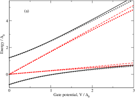
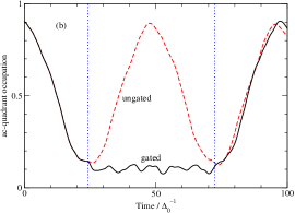
Figure 4: (a) Comparison of the first-order perturbation theory (Equation (12) and Equation (18)) with the exact results. Perturbative results are shown with solid (black) / red (dashed) lines for singlet / triplet states, while the exact results are given as black circles / red diamonds. The agreement is excellent for $|V|<2\Delta_{0}$, while outside this range higher-order corrections must be included. (b) The QD is approximately prepared in the state $|S_{\updownarrow}\rangle$ by applying $V=3\Delta_{0}$. This gate potential is then released and the singlet cycles to a horizontal orientation and back again, as seen by the occupation of the quadrants $ac$ (dashed line). If the gate potential is reapplied during the cycle, the evolution of the singlet is frozen until the potential is released again (solid line). The vertical (blue) dotted lines indicate the times at which the gating potential is first applied and then removed. The ripples in the time-evolution result from the excitation of energy levels outside the lowest multiplet. (c) Exchange coupling $J/\Delta_{0}$ versus $V/\Delta_{0}$. Black circles show the exact results, the dashed line the prediction from perturbation theory.

To illustrate the accuracy of the simple effective Hamiltonian we compare it with the full numerical solutions of the 2-electron problem. The energy eigenvalues vs $V$ for the lowest two singlets and triplets are plotted in Figure 4(a) and we see excellent agreement between the effective model and the real one. The advantage of the approximate model is that we have precise analytic solutions which can be used to derive analytic expressions for all quantities of interest.

3 Singlet-triplet filtering

The analytic expressions for the energies of the singlet states (12) and the triplet states (18) give us a complete picture for the system’s time dependence. In particular they produce the phenomenon of “singlet-triplet filtering”, studied in detail in Ref. [20] for the case of $V=0$. This is a consequence of the very different dynamics displayed by the singlet and triplet states under free evolution. For example, if the system is initialized in the singlet state $|S_{\updownarrow}\rangle$, it will subsequently evolve coherently in time as

$$e^{-iHt}|S_{\updownarrow}\rangle=e^{-i(E_{0S}+V)t}\left(\sin(2\theta)\sin(\omega t)|S_{\leftrightarrow}\rangle+(\cos(\omega t)+i\cos(2\theta)\sin(\omega t))|S_{\updownarrow}\rangle\right),$$ (22)

where $\omega=\sqrt{\Delta_{0}^{2}+[V(1-2p^{bd}_{S_{\updownarrow}})]^{2}}$. The horizontal and vertical components of the state thus cycle periodically in time, and for the specific case of $V=0$ there will be a complete conversion of $|S_{\updownarrow}\rangle$ to $|S_{\leftrightarrow}\rangle$ after a time $t_{R}=\frac{\pi}{2\Delta_{0}}$. In contrast, if the system is initialized in the triplet state $|T_{\updownarrow}\rangle$, its time dependence simply consists of a trivial phase, as the triplet Hamiltonian (17) does not contain tunneling terms between the triplet states. The spin of the initial state can thus be detected, or filtered, by a single charge measurement at $b$ or $d$; the singlet component oscillates periodically with time, while the triplet component stays frozen in position.

We now examine how the presence of the gate potential ($V\neq 0$) alters this picture. When $V(1-2p^{bd}_{S_{\updownarrow}})\gg\Delta_{0}$, $\theta\rightarrow 0$ and $|S_{\updownarrow}\rangle$ becomes effectively the eigenvector of the system and does not evolve. Applying a large gate potential thus has the effect of shutting off the oscillation of the singlet states between the vertical and horizontal configurations. We show this effect in Figure 4(b), by plotting the time-evolution of the system prepared in the state $|S_{\updownarrow}\rangle$ under the full two-electron Hamiltonian (1). In the absence of a gate potential, the singlet periodically cycles between its vertical and horizontal orientations as expected from our effective model. However, reapplying the gate potential freezes the time evolution of the system, which remains halted until the potential is again released.

4 Qubits

We define the two levels of our qubit as vertical singlet-triplet states, i.e. $|0\rangle=|S_{\updownarrow}\rangle$ and $|1\rangle=|T_{\updownarrow}^{0}\rangle$ (both $S_{z}=0$ states). In the regime of strong $V$ this qubit is well-defined, and is highly localized in its vertical configuration. For finite $V$, the eigenvector $|S_{1}\rangle$ has a small contribution of $|S_{\leftrightarrow}\rangle$, as $|\langle S_{\leftrightarrow}|S_{1}\rangle|^{2}\simeq|\frac{\Delta_{0}}{V(1-2p^{bd}_{S_{\updownarrow}})}|^{2}$, but this can be arbitrarily suppressed by controlling $V$. Furthermore, as shown in Figure 2, in the regime of strong $V$ both $|S_{1}\rangle$ and $|T_{1}^{0}\rangle$ become almost degenerate, and so there will be no relative phase between them.

5 Single qubit manipulations

An arbitrary unitary operation on a single qubit can be realized by sequential rotations around two different axes, such as $x$ and $z$. Rotations around the $z$-axis may be simply achieved by the energy splitting $J=E_{0T}-E_{0S}$ between $|S_{1}\rangle$ and $|T_{\updownarrow}^{0}\rangle$ in the regime of $V(1-2p^{bd}_{S_{\updownarrow}})\gg\Delta_{0}$ where the electrons are still strongly localized in their vertical configurations (i.e. $|S_{1}\rangle\approx|S_{\updownarrow}\rangle$), but $J$ does not vanish. This exchange coupling $J$ generates a relative phase between the logical qubits $|0\rangle$ and $|1\rangle$ and thus performs a $z$-rotation. In Figure 4(c) the exchange coupling $J$ is plotted versus $V/\Delta_{0}$. From this figure one can select the appropriate $V$ to give the $J$ that will perform the desired rotation in a given time interval, during which the electrons remain in the vertical configuration.

Rotation around the $x$ axis demands switching between $|0\rangle$ and $|1\rangle$. To do that a gradient of magnetic field $\delta B_{z}$ is required between the vertical corners $ac$. There are two different proposals for generating this gradient magnetic field: (i) polarizing the spin of the nuclei in the bulk [16]; (ii) using permanent micro-magnets [17, 18]. Here, we propose to use permanent micro-magnets near the the corners $ac$ as shown in Figure 1(a). To perform an $x$ rotation, one has to push the electrons close to the micro-magnets to sense $\delta B_{z}$ by applying a strong positive bias to the gates $G_{a}$ and $G_{c}$, which may be the micro-magnets themselves. The gradient $\delta B_{z}$ rotates a single electron around the $z$ axis and consequently switches between a singlet and a triplet state.

6 Initialization

An initial qubit state may be created by injecting a spin-up electron into corner $a$ and a down-spin electron into corner $c$, while holding $V$ large enough to ensure that the electrons remain well-localized in these corners. The electrons are thus created in the state $|+\rangle=(|0\rangle+|1\rangle)/\sqrt{2}$. Other initial states may then be generated with single-qubit transformations, described earlier.

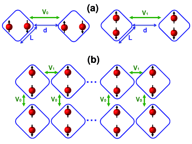
Figure 5: (a) Capacitive interaction of different charge configurations between two square quantum dots of size $L$ and distance $d$. (b) A two dimensional array of QDs for producing cluster states. Different horizontal and vertical interactions results in different two-qubit gates which can be compensated by local rotations.

7 Two-qubit entangling gate

Apart from single qubit unitary operations, the more challenging two-qubit quantum gates are also essential for universal quantum computation [19]. We consider two square QDs, each containing two electrons encoding a singlet-triplet qubit as described above. Interaction between the left and right qubits is mediated through the electrostatic Coulomb repulsion, as shown in Figure 5(a), which is independent of the spin states. Due to symmetry there are three independent electrostatic energies for the four possible spatial configurations of electrons in two QDs (i.e. $\updownarrow\updownarrow$, $\updownarrow\leftrightarrow$, $\leftrightarrow\updownarrow$ and $\leftrightarrow\leftrightarrow$), where one of them can also set to be zero (overall energy shift). Therefore, as schematically shown in Figure 5(a), we can write the interaction between the two QDs as

$$H_{I}=\sum_{k,l=S,T}\left(u_{0}|k_{\leftrightarrow},l_{\leftrightarrow}\rangle\langle k_{\leftrightarrow},l_{\leftrightarrow}|+u_{1}|k_{\updownarrow},l_{\updownarrow}\rangle\langle k_{\updownarrow},l_{\updownarrow}|\right),$$ (23)

where $u_{0},u_{1}>0$ account for the electrostatic Coulomb energies in the configurations $\leftrightarrow\leftrightarrow$ and $\updownarrow\updownarrow$ respectively while the interactions of configurations $\updownarrow\leftrightarrow$ and $\leftrightarrow\updownarrow$ are chosen as the offset. By treating the electrons as classical point charges localized in the corners of the square confining potential, one can estimate $u_{0}$ and $u_{1}$ as functions of the dot size $L$ and their distance $d$ (see Figure 5(a)). In fact, the leading terms in Coulomb energies $u_{0}$ and $u_{1}$ are second order in $L/d$ giving

$$u_{0}=\frac{e^{2}}{4\pi\epsilon_{0}\epsilon_{r}d}\{3(\frac{L}{d})^{2}+\mathcal{O}((L/d)^{3})\}$$ (24)

$$u_{1}=\frac{e^{2}}{4\pi\epsilon_{0}\epsilon_{r}d}\{(\frac{L}{d})^{2}+\mathcal{O}((L/d)^{3})\},$$ (25)

where $\epsilon_{0}$ is the vacuum permittivity and $\epsilon_{r}=10.8$ is the dielectric constant of GaAs.

The Hamiltonian of the whole system then becomes $H_{\mathrm{tot}}=H_{L}+H_{R}+H_{I}$, where $H_{L}$ and $H_{R}$ are given by Equation (4) for the left and right QDs. The existence of $H_{I}$ changes the eigenstates of the system, and therefore the dynamics of Equation (22). To preserve the picture in which triplets do not evolve and singlet states rotate according to Equation (22), we should keep $u_{0},u_{1}\ll\Delta_{0}$ by fabricating the QDs relatively far apart. As discussed in Appendix A the choice of $u_{0},u_{1}\sim 0.1\Delta_{0}$ is sufficient to retain this picture.

To have a two-qubit quantum gate, we first assume that $V$ is large and both qubits are initialized in an arbitrary superposition of $|S_{\updownarrow}\rangle$ and $|T_{\updownarrow}^{0}\rangle$. To operate the two-qubit gate, $V$ is set to zero. As $u_{0},u_{1}\ll\Delta_{0}$ the interaction Hamiltonian does not play an important role during this evolution, and so the dynamics is mainly governed by $H_{0}=H_{L}+H_{R}$, in which the triplets do not evolve and singlets rotate according to Equation (22) with $V=0$. After time $t=t_{R}$ the evolution is again frozen by setting $V$ to a negative value which keeps the electrons in the horizontal configuration for an interaction time period of $t_{I}$, during which the system evolves under the action of $H_{I}$ alone. The potential barriers are then again removed (i.e. $V$ is set to zero) for another period of $t=t_{R}$ to return the electrons to their initial positions. One can write the total evolution operator as

$$U(t_{I})=e^{-iH_{0}t_{R}}e^{-iH_{I}t_{I}}e^{-iH_{0}t_{R}}.$$ (26)

Over the interaction time $t_{R}<t<t_{R}+t_{I}$, each spatial configuration determined by the spin state of electrons has its own electrostatic energy, and thus the time evolution gives different phases to every state. One may easily verify that

$$U(t_{I})|S_{\updownarrow},S_{\updownarrow}\rangle = e^{-iu_{0}t_{I}}|S_{\updownarrow},S_{\updownarrow}\rangle$$ (27)

$$U(t_{I})|S_{\updownarrow},T_{\updownarrow}\rangle = -|S_{\updownarrow},T_{\updownarrow}\rangle$$ (28)

$$U(t_{I})|T_{\updownarrow},S_{\updownarrow}\rangle = -|T_{\updownarrow},S_{\updownarrow}\rangle$$ (29)

$$U(t_{I})|T_{\updownarrow},T_{\updownarrow}\rangle = e^{-iu_{1}t_{I}}|T_{\updownarrow},T_{\updownarrow}\rangle.$$ (30)

For $t_{I}=\frac{\pi}{u_{0}+u_{1}}$, this evolution realizes an entangling two-qubit gate such that its application to the state $|++\rangle$ maximally entangles the two qubits. Moreover, this gate can be converted to the standard controlled $z$ ($CZ$) gate by two local rotations around the $z$ axis with the angle $\frac{\pi}{2(u_{0}+u_{1})}$.

8 Readout

In our mechanism, single qubit measurement in the computational $z$ basis is the singlet-triplet measurement of the electron pair in the QD. This can be achieved by setting $V$ to zero, thereby allowing tunneling from vertical to horizontal configurations for the singlet (triplet states are unable to tunnel from vertical to horizontal as there are no tunneling elements between these states). A single charge detection then fulfills the singlet-triplet measurement [20], as explained in Section 3. Single qubit measurement in any other basis can be simply reduced to a $z$ measurement by applying proper local rotations.

9 Applications

Universal quantum computation can be achieved in two dimensional network of qubits, which can be prepared in a highly entangled state termed a cluster state [21]. To prepare a cluster state we need a two-dimensional array of qubits all initially prepared in $|+\rangle$ states. Then a homogeneous action of $CZ$ gates between all neighboring qubits generates a cluster state, on which measurement-based quantum computation can be realized by local rotations and single qubit measurements [21]. Such an array of QDs is shown in Figure 5(b). Note that when electrons are frozen in their locations, the electrostatic interactions only give a global phase. In this structure when the system is released for a global gate operation, the type of the gate that acts on rows is different from the one acting on columns, unless $u_{0}=u_{1}$. However, these gates can be locally transformed to $CZ$ gates, and thus the outcome is still a cluster state and can be used for measurement-based quantum computation. Note that in an array of double dots used to realize a two-qubit gate, one has to change the charge configurations to $(0,2)$, which makes the left and right neighbor qubits experience asymmetric interactions, thereby prohibiting simultaneous identical gates.

10 Practicality and time scales

In this section we estimate the parameters of the system and explore the experimental feasibility of our proposal. For QDs of side-length $L=400$ nm, we have $\Delta_{0}\simeq 20\mu$eV. Separating the QDs so that $u_{0}+u_{1}\simeq 2\mu$eV guarantees the validity of Equation (22) to very high precision, as $\Delta_{0}/(u_{0}+u_{1})\simeq 10$. The operation time of our two-qubit gate is $2t_{R}+t_{I}=\frac{\pi\hbar}{\Delta_{0}}+\frac{\pi\hbar}{u_{0}+u_{1}}$. Using the above values yields an operation time of $2t_{R}+t_{I}=12$ ns. The spacing between the QDs ($d$) corresponding to this choice of physical parameters can be calculated from Equation (24), giving a value of $d\simeq 3.6\mu$m.

To determine the temperatures in which the system can operate one has to estimate the energy gap of the system. From Figure 2 one can see that the energy gap between the singlet and triplet subspace is $\Delta E\simeq\Delta_{0}$. For the system to operate safely the temperature should be below the energy gap. Using the above parameters for a square dot of size $L=400$ nm in which $\Delta_{0}\simeq 20\mu$eV, one can evaluate the energy gap as $\Delta E\simeq 200$ mK which is larger than the typical temperatures ($\sim 100$ mK) achievable with current dilution fridges. This clearly shows that the proposed mechanism can be realized with existing technology.

11 Decoherence and robustness

A major obstacle for realizing two qubit gates through capacitive interaction in double dot systems is the very short charge dephasing time ($\sim 1$ ns). Such a short time scale is due to the interaction between the electric dipole $\overrightarrow{\mathbf{p}}$ of the two electrons with the random fluctuating electric field $\overrightarrow{\mathbf{E}}(t)$ (namely $U=-\overrightarrow{\mathbf{p}}.\overrightarrow{\mathbf{E}}(t)$). To realize a two-qubit quantum gate in double dot systems one can use the electrostatic coupling between the two neighboring double dots which give different phases to singlets and triplets according to their different charge configurations. Since the charge configurations of the singlets and triplets are quite similar for the $(1,1)$ configuration the time scale of the two qubit gate becomes too long (for instance it is $\sim 150$ ns in the realization of Ref. [11]). One can speed up this process significantly, even up to $\sim 20$ ns [10], by giving more offset energy to one of the dots in order to convert the singlet charge configuration to $(2,0)$, leaving one of the dots empty, to make the capacitive interaction stronger. However, this produces significant charge dephasing, as singlets and triplets have different electric dipole moments (due to the asymmetric charge configuration $(0,2)$ of the singlets) and interact differently with electric field fluctuations. In contrast, in our square QD proposal the charge configuration always remains symmetric with zero electric dipole moment. Hence, the leading term for charge dephasing is quadrupolar, giving a much longer charge dephasing time.

The hyperfine interaction between the electrons and nuclei in the bulk is the main source of decoherence in QDs. To compensate this effect we may use the recently-implemented idea of multiple-pulse echo sequence [6]. In this technique the quantum states of the two electrons are swapped through exchange interaction regularly, allowing decoherence times of $T_{2}\sim 260\mu$s. As mentioned in the previous section, for dots with the size $L=400$ nm, we have $\Delta_{0}\simeq 20\mu$eV and fabricating the dots with a spacing of $d\simeq 3.5\mu$m gives $\Delta_{0}/(u_{0}+u_{1})\simeq 10$. These parameters imply that the two-qubit operation time will be $2t_{R}+t_{I}\simeq 12$ ns which allows for of the order of $10^{5}$ operations within the coherence time of the system. Even in the absence of regular exchange of quantum states, the hyperfine interaction between the electrons and nuclei in the bulk is at least two orders of magnitude smaller than $\Delta_{0}$ [20], and one order of magnitude less than $u_{0}+u_{1}$. This guarantees that it has no significant effect over the proposed fast dynamics ($\sim$ 12 ns) although the coherence time is then limited to 1 $\mu s$ [9] and thus the number of operation reduces to $\sim 10^{3}$.

Another major of imperfection in singlet-triplet double QD systems is due to the gate voltage fluctuations [22]. This makes the tunneling between the two dots noisy which then results in fluctuations in spin exchange coupling which is $J\sim t^{2}/U$ (for tunneling $t$ and on-site energy $U$). As tunneling in double dot systems is directly controlled by gate voltages while the on-site energy is independently determined by the Coulomb interaction, the spin exchange coupling fluctuates in time with the tunneling [22]. In our square QD system, however, the exchange coupling $J=E_{T_{\updownarrow}}(V)-E_{S_{1}}(V)$ is determined by $J\sim\Delta_{0}^{2}/V$. So, in the large $V$ limit, which we use for the single qubit gate operations, the fluctuations of the gate voltage $V$ appear only in the denominator and $\Delta_{0}$ is independent of $V$ to first order. Thus we expect less sensitivity to gate voltages in our scheme.

So far we have assumed that $V$ can be instantaneously switched on and off at desired times. In reality gate voltages cannot jump instantly, and so $V$ varies gradually. One can estimate the gradual switching error by assuming that $V$ is switched off (or on) linearly over a period of $\tau$. For instance, in Equation (22) a linear switching of $V$ over the time period $t=t_{R}$ to $t=t_{R}+\tau$ produces an error equal to $\sin^{2}(\frac{\Delta_{0}\tau}{2})\approx\frac{\Delta_{0}^{2}\tau^{2}}{4}$. In particular, for QDs of size $L=400$ nm, (i.e. $\Delta_{0}=20\mu$eV) a gradual switching with duration $\tau=10$ ps induces less than $2\%$ error in our desired state.

12 Alternative realization

Apart from GaAs technology, one can also realize our quantum cellular automata using the silicon atom dangling bonds on hydrogen terminated silicon crystal surface [23, 24]. The four coupled QDs located in a ring, hosting two highly interacting electrons (fully capable for achieving our spin filtering dynamics) have been realized experimentally [24]. The isotopically purified silicon provides very long decoherence time ($T_{2}$ exceeding 200 $\mu s$) as the nuclear spin interaction is practically eliminated, and a charge dephasing time of $\sim 200$ns has been measured for charge qubits in Si double QDs [25].

13 Conclusions

We have shown that the singlet and triplet states of a pair of electrons held in a square QD can be used as a rapid and deterministically-controlled qubit. Introducing electrostatic interactions between neighboring qubits allows two-qubit entangling gates to be constructed, thus enabling universal quantum computation, with particular suitability to its measurement-based version. The extra charge orbital in our system enables the fundamental issue of short charge dephasing time of singlet-triple qubits in double dots to be tackled by having zero dipole moment. Hence the leading interaction with the environment is quadrupolar, resulting in much longer charge coherence. The architecture was inspired by classical cellular automata implementations [1, 2] thereby linking them to the quantum realm and providing a path for quantum-classical integrability in computer technology. While singlet-triplet qubits have already been realized in double dots, our proposal makes a number of advances, namely: (i) no electric dipoles at any stage (potentially much longer coherence); (ii) symmetric gate operations; (iii) no relative phases during the storage; and (iv) non-adiabatic (i.e. fast) operation which could become preferable in view of the continually improving speed of control electronics; (v) less sensitivity to gate voltage fluctuations. We should emphasize that as well as the single QD geometry we have presented here, our results are also applicable with minor modifications to the four-dot structure studied experimentally in Ref. [26].

Appendix A Two neighboring QDs

In the paper we have introduced the interaction between two neighboring QDs which interact through capacitive Coulomb repulsion. The form of the interaction Hamiltonian is given by $H_{I}$ in Equation (23). The existence of $H_{I}$ changes the eigenvectors of the system and therefore may affect the system’s dynamics. To quantify the effect of this interaction on the spectrum of $H_{0}=H_{L}+H_{R}$, we compute the modified eigenstates of the whole system $H_{tot}$ when $H_{I}$ is treated perturbatively. Within this regime the new relevant unnormalized eigenvectors are given to first order by

$$|S_{1},S_{1}\rangle \rightarrow |S_{1},S_{1}\rangle+a|S_{1},S_{2}\rangle+a|S_{2},S_{1}\rangle-b|S_{2},S_{2}\rangle$$ (31)

$$|S_{1},S_{2}\rangle \rightarrow \frac{|S_{1},S_{2}\rangle+|S_{2},S_{1}\rangle}{\sqrt{2}}-a\sqrt{2}(|S_{1},S_{1}\rangle-|S_{2},S_{2}\rangle)$$ (32)

$$|S_{2},S_{1}\rangle \rightarrow \frac{|S_{1},S_{2}\rangle-|S_{2},S_{1}\rangle}{\sqrt{2}}$$ (33)

$$|S_{2},S_{2}\rangle \rightarrow |S_{2},S_{2}\rangle+b|S_{1},S_{1}\rangle-a|S_{1},S_{2}\rangle-a|S_{2},S_{1}\rangle$$ (34)

$$|S_{1},T_{0}\rangle \rightarrow |S_{1},T_{\updownarrow}^{0}\rangle-c|S_{2},T_{\updownarrow}^{0}\rangle$$ (35)

$$|T_{0},S_{1}\rangle \rightarrow |T_{\updownarrow}^{0},S_{1}\rangle-c|T_{\updownarrow}^{0},S_{2}\rangle$$ (36)

$$|S_{2},T_{0}\rangle \rightarrow |S_{2},T_{\updownarrow}^{0}\rangle+c|S_{1},T_{\updownarrow}^{0}\rangle$$ (37)

$$|T_{0},S_{2}\rangle \rightarrow |T_{\updownarrow}^{0},S_{2}\rangle+c|T_{\updownarrow}^{0},S_{1}\rangle$$ (38)

where,

$$a=\frac{u_{0}-u_{1}}{8\Delta_{0}},\ \ b=\frac{u_{0}+u_{1}}{16\Delta_{0}},\ \ c=\frac{u_{1}}{4\Delta_{0}}.$$ (39)

Tuning $u_{0},u_{1}\simeq 0.1\Delta_{0}$ guarantees that the oscillation between $|S_{\updownarrow}\rangle$ and $|S_{\leftrightarrow}\rangle$ remains valid up to a very high fidelity ($>0.9$).

References

References

- [1] C. S. Lent, P. D. Tougaw, and W. Porod, Appl. Phys. Lett. 62, 714 (1993); E. P. Blair and C. S. Lent J. Appl. Phys 113, 124302 (2013).
- [2] R. P. Cowburn and M. E. Welland, Science 287, 1466 (2000).
- [3] G. Toth and C. S. Lent, Phys. Rev. A 63, 052315 (2001).
- [4] G. Toth, C. S. Lent, App. Phys. 89 7943 (2001); J. H. Jefferson, M. Fearn, D. L. J. Tipton, and T. P. Spiller Phys. Rev. A 66, 042328 (2002).
- [5] D. Loss and D. P. DiVincenzo, Phys. Rev. A 57, 120 (1998).
- [6] H. Bluhm et al., Nat. Phys. 7, 109 (2011).
- [7] J. M. Taylor et al., Phys. Rev. B 76, 035315 (2007).
- [8] R. Hanson, G. Burkard, Phys. Rev. Lett.98, 050502 (2007).
- [9] J. R. Petta et al., Science 309, 2180 (2005).
- [10] I. van Weperen, B. D. Armstrong, E. A. Laird, J. Medford, C. M. Marcus, M. P. Hanson, and A. C. Gossard, Phys. Rev. Lett. 107, 030506 (2011).
- [11] M. d. Shulman, O. E. Dial, S. P. Harvey, H. Bluhm, V. Umansky, A. Yacoby, Science 336, 202 (2012).
- [12] J. M. Taylor et al., Nature Phys. 1, 177 (2005).
- [13] D. K. L. Oi, S. G. Schirmer, A. D. Greentree, and T. M. Stace, Phys. Rev. B 72, 075348 (2005).
- [14] W. A. Coish and D. Loss, Phys. Rev. B 72, 125337 (2005).
- [15] C. E. Creffield, W. Häusler, J. H. Jefferson, and S. Sarkar, Phys. Rev. B 59, 10719 (1999).
- [16] S. Foletti et al., Nature Phys. 5, 903 (2009).
- [17] M. Pioro-Ladriere et al., Nature Phys. 4, 776 (2008).
- [18] F. Forster, M. Mühlbacher, D. Schuh, W. Wegscheider, and S. Ludwig, Phys. Rev. B 91, 195417 (2015).
- [19] M. J. Bremner et al., Phys. Rev. Lett. 89, 247902 (2002).
- [20] J. G. Coello, A. Bayat, S. Bose, J. H. Jefferson, C. E. Creffield, Phys. Rev. Lett. 105, 080502 (2010).
- [21] H. J. Briegel, et al., Nature Physics 5, 19 (2009).
- [22] X. Hu and S. Das Sarma, Phys. Rev. Lett. 96, 100501 (2006).
- [23] T.-C. Shen, C. Wang, G. C. Abeln, J. R. Tucker, J. W. Lyding, Ph. Avouris, and R. E. Walkup, Science 268, 1590 (1995); P. G. Piva, G. A. DiLabio, J. L. Pitters, J. Zikovsky, M. Rezeq, S. Dogel, W. A. Hofer, and R. A. Wolkow, Nature 435, 658 (2005).
- [24] M. B. Haider, J. L. Pitters, G. A. DiLabio, L. Livadaru, J. Y. Mutus, and R. A. Wolkow, Phys. Rev. Lett. 102, 046805 (2009); J. L. Pitters, L. Livadaru, M. B. Haider, and R. A. Wolkow, J. Chem. Phys. 134, 064712 (2011).
- [25] J. Gorman, D. G. Hasko, D. A. Williams, Phys. Rev. Lett. 95, 090502 (2005).
- [26] K. D. Petersson, C. G. Smith, D. Anderson, P. Atkinson, G. A. C. Jones, and D. A. Ritchie, Phys. Rev. Lett. 103, 016805 (2009).