Which galaxies dominate the neutral gas content of the Universe?

Abstract

We study the contribution of galaxies with different properties to the global densities of star formation rate (SFR), atomic (HI) and molecular hydrogen (H₂) as a function of redshift. We use the GALFORM model of galaxy formation, which is set in the $\Lambda$CDM framework. This model includes a self-consistent calculation of the SFR, which depends on the H₂ content of galaxies. The predicted SFR density and how much of this is contributed by galaxies with different stellar masses and infrared luminosities are in agreement with observations. The model predicts a modest evolution of the HI density at $z<3$, which is also in agreement with the observations. The HI density is predicted to be always dominated by galaxies with SFR$<1M_{\odot}\,\rm yr^{-1}$. This contrasts with the H₂ density, which is predicted to be dominated by galaxies with SFR$>10M_{\odot}\,\rm yr^{-1}$ at $z>1$. Current high-redshift galaxy surveys are limited to detect carbon monoxide in galaxies with ${\rm SFR}\gtrsim 30M_{\odot}\,\rm yr^{-1}$, which in our model make up, at most, $20$% of the H₂ in the universe. In terms of stellar mass, the predicted H₂ density is dominated by massive galaxies, $M_{\rm stellar}>10^{10}\,M_{\odot}$, while the HI density is dominated by low mass galaxies, $M_{\rm stellar}<10^{9}\,M_{\odot}$. In the context of upcoming neutral gas surveys, we suggest that the faint nature of the galaxies dominating the HI content of the Universe will hamper the identification of optical counterparts, while for H₂, we expect follow up observations of molecular emission lines of already existing galaxy catalogues to be able to uncover the H₂ density of the Universe.

1 Introduction

Observations of local and high-redshift galaxies indicate that stars form from molecular gas, albeit with a low efficiency (e.g. Bigiel et al. 2008; Genzel et al. 2010). On scales of kilo-parsecs, this fact is observed as a close to linear correlation between the star formation rate (SFR) surface density and the surface density of molecular hydrogen (H₂) (Bigiel et al. 2008; Bigiel et al. 2010; Leroy et al. 2008; Schruba et al. 2011). The observational and theoretical evidence gathered point to a scenario in which gas cools down and becomes molecular before collapsing and fragmenting to form stars, with the small efficiency explained as being due to self-regulation as the results of star formation at the level of giant molecular clouds. Therefore, the presence of neutral gas by itself does not guarantee star formation (see Kennicutt & Evans 2012 for a recent review). This emphasises the importance of H₂ as the main tracer of the dense regions where stars form. Regarding the atomic hydrogen (HI), studies of local Universe galaxies show a strong correlation between the HI mass and the stellar mass, indicating that the evolution of the two quantities is related (e.g. Catinella et al. 2010; Cortese et al. 2011; Huang et al. 2012). In addition, the morphology of the atomic hydrogen in galaxies is closely related to baryonic processes such as gas accretion and outflows in galaxies (Fraternali et al. 2002; Oosterloo et al. 2007; Boomsma et al. 2008). Observations have shown that the presence of stellar driven outflows depends on the star formation rate density (e.g. Chen et al. 2010; Newman et al. 2012). Lagos et al. (2013) and Creasey et al. (2013), using hydrodynamical modelling of the growth of supernovae driven bubbles in the ISM of galaxies, show that the fundamental property setting the outflow rate is the gas surface density, as it affects both the SFR, which sets the energy input from supernovae, and the time bubbles take to escape the galaxy disk.

All of the evidence above points to the fact that a key step in understanding galaxy formation is the observation of multiple gas phases in the ISM and their relation to the presence of SF. In particular, observations of atomic and molecular hydrogen, which make up most of the mass in the interstellar medium (ISM) of galaxies, are key to understanding how SF proceeds and how gas abundances can be linked to accretion and outflow of gas. Only through tracing both molecular and atomic gas components at the same time as the SFR and stellar mass in galaxies will we be able to develop a better understanding of the processes of SF and feedback and to put strong constraints on galaxy formation simulations.

Currently, observational constraints on the HI and H₂ contents of galaxies are available for large local samples, and for increasingly large samples at high-redshift. In the case of HI, accurate measurements of the $21$ cm emission in large surveys of local galaxies have been presented by Zwaan et al. (2005) using the HI Parkes All-Sky Survey (HIPASS; Meyer et al. 2004) and by Martin et al. (2010) using the Arecibo Legacy Fast ALFA Survey (ALFALFA; Giovanelli et al. 2005). The global HI mass density at $z=0$ has been estimated from these surveys to be in the range $\Omega_{\rm HI}=3.6-4.2\times 10^{-4}$, with little evolution up to $z\approx 5$ (e.g. Péroux et al. 2003; Noterdaeme et al. 2009). This lack of evolution is fundamentally different from the evolution inferred in the SFR density, which shows a strong increase from $z\approx 0$ to $z\approx 2-3$, followed by a slow decline to higher redshifts (e.g. Madau et al. 1996; Lilly et al. 1996; Hopkins & Beacom 2006).

A plausible explanation for the different evolution seen in the SFR and HI densities is that HI is not the direct fuel of SF but instead this gas still needs to cool down further to form stars. This indicates that in order to better understand SF and galaxy evolution, good observations of the denser gas in the ISM, i.e. H₂, are required. Molecular hydrogen is commonly traced by the ${}^{12}\rm CO$ (hereafter ‘CO’) molecule, which is the second most abundant molecule after H₂ and is easily excited. However, direct CO detections are very scarce and complete samples are limited to the local Universe. Keres et al. (2003) reported the first attempt to derive the local $\rm CO(1-0)$ luminosity function from which they inferred the H₂ mass function and the local $\Omega_{\rm H_{2}}=1.1\pm 0.4\times 10^{-4}\,h^{-1}$, adopting a Milky-Way type $\rm CO(1-0)$-H₂ conversion factor. It has not yet been possible to estimate the cosmic H₂ abundance at high redshift. Observational samples that detect CO at high-redshifts are limited to moderately and highly star-forming galaxies with SFR$\gtrsim 20\,M_{\odot}\,\rm yr^{-1}$ (Tacconi et al. 2013; Carilli & Walter 2013). To estimate a density of H₂ from these galaxies is difficult given the selection effects and volume corrections. Recently, Berta et al. (2013) inferred the molecular gas mass function at high-redshift by using the ratio between the UV to mid-IR emission and its empirical relation to the molecular gas mass (Nordon et al., 2013). However, these estimates are subject to the uncertain extrapolation of empirical relations to galaxies and redshifts where they have not been measured. For these reasons the construction of representative samples of H₂ in galaxies is still an unfinished task that is crucial to our understanding of galaxy formation.

From the theoretical point of view, more sophisticated treatments of SF and its relation to the abundance of HI and H₂ have only recently started to be explored in ab-initio cosmological galaxy formation simulations (e.g. Fu et al. 2010; Cook et al. 2010; Lagos et al. 2011b; Kuhlen et al. 2012; Duffy et al. 2012a; Popping et al. 2013a), as well as in simulations of individual galaxies (e.g. Gnedin et al. 2009; Pelupessy & Papadopoulos 2009; Kim et al. 2011; Mac Low & Glover 2012). The improved modelling of the ISM and SF in galaxies that has been applied in cosmological galaxy formation simulations has allowed a better understanding of the neutral content of galaxies; for instance, of the effect of H₂ self-shielding on the column density distribution of HI (Altay et al. 2011; Duffy et al. 2012a), the lack of evolution of the global HI density (Lagos et al. 2011a; Davé et al. 2013), and the increasing molecular gas-fractions of galaxies with redshift (Obreschkow & Rawlings 2009; Lagos et al. 2012; Fu et al. 2012).

The issue motivating this paper is the contribution of star-forming galaxies of different properties to the atomic and molecular gas content of the Universe. Note that this question is similar to asking about the steepness of the faint-end of the gas and stellar mass functions; i.e. the steeper the mass function, the larger the contribution from low-mass galaxies to the total density of mass in the Universe. This exercise is important for two reasons. First, blind CO surveys are very challenging and expensive. For instance, the Atamaca Large Millimeter Array can easily detect galaxies at high-redshift (e.g. Vieira et al. 2013; Hodge et al. 2013), but has the downside of having a very small field of view ($<1$ arcmin), which is not ideal for large surveys. A possible solution is to follow-up samples of galaxies selected by SFR or stellar mass in molecular emission, which can give insight into the relation between SF and the different gas phases in the ISM. Second, because a key science driver of all large HI programs is to understand how the HI content relates to multi-wavelength galaxy properties (see for instance the accepted proposals of the ASKAP HI All-Sky Survey , WALLABY, and the Deep Investigation of Neutral Gas Origins survey, DINGO, Johnston et al. 2008). DINGO will investigate this directly as it overlaps with the Galaxy And Mass Assembly multi-wavelength survey (Driver et al., 2009).

In this paper we bring theoretical models a step closer to the observations and examine how star-forming galaxies of different properties contribute to the densities of SFR, atomic and molecular hydrogen, to inform future neutral gas galaxy surveys about the expected contribution of star-forming galaxies to the HI and H₂ contents of the Universe. We also seek to understand how far we currently are from uncovering most of the gas in galaxies in the Universe. For this study we use three flavours of the semi-analytical model GALFORM in a $\Lambda$CDM cosmology (Cole et al. 2000), namely those of Lagos et al. (2012), Gonzalez-Perez et al. (2013), and Lacey et al. (2014, in prep.). The three models include the improved treatment of SF implemented by Lagos et al. (2011b). This extension explicitly splits the hydrogen content of the ISM of galaxies into HI and H₂. The advantage of using three different flavours of GALFORM is the ability to characterise the robustness of the trends found. The outputs of the three models shown in this paper will be publicly available from the Millennium database (detailed in Appendix C).

This paper is organised as follows. In $\S 2$ we present the galaxy formation model and describe the realistic SF model used. We also describe the main differences between the three models that use this SF law and the dark matter simulations used. In $\S 3$ we compare the model predictions with observations of the evolution of the SFR, HI and H₂ densities, and the SF activity in normal and highly star-forming galaxies. None of the observations in $\S 3$ were used to constrain model parameters, and therefore provide independent verifications of the predictions of the models. Given the success of our model predictions, we investigate the contribution from star-forming galaxies to the densities of HI and H₂ in $\S 4$ and discuss the physical drivers of the predictions. In $\S 5$ we discuss the implications of our predictions for the next generation of HI and H₂ surveys and present the main conclusions in $\S 6$.

2 Modelling the two-phase cold gas in galaxies

In this section, we briefly describe the main aspects of the GALFORM semi-analytical model of galaxy formation and evolution (Cole et al., 2000), focusing on the key features of the three flavours adopted in this study, which are described in Lagos et al. (2012; hereafter ‘Lagos12’), Gonzalez-Perez et al. (2013; hereafter ‘Gonzalez-Perez14’) and Lacey et al. (2014; hereafter ‘Lacey14’).

The three GALFORM models above take into account the main physical processes that shape the formation and evolution of galaxies. These are: (i) the collapse and merging of dark matter (DM) halos, (ii) the shock-heating and radiative cooling of gas inside DM halos, leading to the formation of galactic disks, (iii) quiescent star formation in galaxy disks, (iv) feedback from supernovae (SNe), from active galactic nucleus (AGN) heating and from photo-ionization of the inter-galactic medium (IGM), (v) chemical enrichment of stars and gas, and (vi) galaxy mergers driven by dynamical friction within common DM halos which can trigger bursts of SF, and lead to the formation of spheroids (for a review of these ingredients see Baugh 2006; Benson 2010). Galaxy luminosities are computed from the predicted star formation and chemical enrichment histories using a stellar population synthesis model (see Gonzalez-Perez et al. 2013).

The three flavours of GALFORM used in this study adopt the same SF law, which is a key process affecting the evolution of the gas content of galaxies. In $\S$ 2.1 we describe this choice of SF law and how this connects to the two-phase ISM, in $\S$ 2.2 we describe the differences between the three flavours of GALFORM and in $\S$2.3 we briefly describe the dark matter simulations used for this study and the cosmological parameters adopted.

2.1 Interstellar medium gas phases and the star formation law

The three flavours of GALFORM used in this study adopt the SF law developed in Lagos et al. (2011a, hereafter ‘L11’), in which the atomic and molecular phases of the neutral hydrogen in the ISM are explicitly distinguished. L11 found that the SF law that gives the best agreement with the observations without the need for fine tunning is the empirical SF law of Blitz & Rosolowsky (2006). Given that the SF law has been well constrained in spiral and dwarf galaxies in the local Universe, L11 decided to implement this molecular-based SF law only in the quiescent SF mode (SF due to gas accretion onto the disk), keeping the original prescription of Cole et al. (2000) for starbursts (driven by galaxy mergers and global disk instabilities). We provide more details below.

Quiescent Star Formation. The empirical SF law of Blitz & Rosolowsky has the form,

$$\Sigma_{\rm SFR}=\nu_{\rm SF}\,\rm f_{\rm mol}\,\Sigma_{\rm gas},$$ (1)

where $\Sigma_{\rm SFR}$ and $\Sigma_{\rm gas}$ are the surface densities of SFR and total cold gas mass (molecular and atomic), respectively, $\nu_{\rm SF}$ is the inverse of the SF timescale for the molecular gas and $\rm f_{\rm mol}=\Sigma_{\rm mol}/\Sigma_{\rm gas}$ is the molecular to total gas mass surface density ratio. The molecular and total gas contents include the contribution from helium, while HI and H₂ only include hydrogen (which in total corresponds to a fraction $X_{\rm H}=0.74$ of the overall cold gas mass). The ratio $\rm f_{\rm mol}$ depends on the internal hydrostatic pressure as $\Sigma_{\rm H_{2}}/\Sigma_{\rm HI}=\rm f_{\rm mol}/(f_{\rm mol}-1)=(P_{\rm ext}/P_{0})^{\alpha}$. To calculate $\rm P_{\rm ext}$, we use the approximation from Elmegreen (1989), in which the pressure depends on the surface density of gas and stars. We give the values of the parameters involved in this SF law in $\S$ 2.2.

Starbusts. In starbursts the SF timescale is proportional to the bulge dynamical timescale above a minimum floor value and involves the whole cold gas content of the galaxy, $\rm SFR={\it M}_{\rm cold}/\tau_{\rm SF}$ (see Granato et al. 2000 and Lacey et al. 2008 for details). The SF timescale is defined as

$$\tau_{\rm SF}=\rm max(\tau_{\rm min},f_{\rm dyn}\tau_{\rm dyn}),$$ (2)

where $\tau_{\rm dyn}$ is the bulge dynamical timescale, $\tau_{\rm min}$ is a minimum duration of starbursts and $f_{\rm dyn}$ is a parameter. We give the values of the parameters involved in this SF law in $\S$ 2.2.

Throughout this work we assume that in starbursts, the cold gas content is fully molecular, $\rm f_{\rm mol}=1$. Note that this is similar to assuming that the relation between the ratio $\Sigma_{\rm H_{2}}/\Sigma_{\rm HI}$ and $P_{\rm ext}$ holds in starbursts given that large gas and stellar densities lead to $\rm f_{\rm mol}\approx 1$. Throughout the paper we refer to galaxies going through a starburst, which are driven by galaxy mergers or disk instabilities, as ‘starbursts’.

Another key component of the ISM in galaxies is dust. To compute the extinction of starlight we adopt the method described in Lacey et al. (2011) and Gonzalez-Perez et al. (2012), which uses the results of the physical radiative transfer model of Ferrara et al. (1999) to calculate the dust attenuation at different wavelength. The dust model assumes a two-phase interstellar medium, with star-forming clouds embedded in a diffuse medium. The total mass of dust is predicted by GALFORM self-consistently from the cold gas mass and metallicity, assuming a dust-to-gas ratio which is proportional to the gas metallicity. The radius of the diffuse dust component is assumed to be equal to the half-mass radius of the disk, in the case of quiescent SF, or the bulge, in the case of starbursts. With this model, we can estimate the attenuation in the wavelength range from the far-ultraviolet (FUV) to the near-infrared (IR), including emission lines. In GALFORM the extinction for emission lines is calculated as due to the diffuse dust component only, so it is the same as the extinction of older stars (i.e. outside their birth clouds) at the same wavelength. We define the total IR luminosity as the total luminosity emitted by interstellar dust, free from contamination by starlight, which approximates to the integral over the rest-frame wavelength range 8$-$1000 $\mu$m.

2.2 Differences between the Lagos12, Gonzalez-Perez14 and Lacey14 models

The Lagos12 model is a development of the model originally described in Bower et al. (2006), which was the first variant of GALFORM to include AGN feedback as the mechanism suppressing gas cooling in massive halos. The Lagos12 model assumes a universal initial mass function (IMF), the Kennicutt (1983) IMF. Lagos12 extend the model of Bower et al. by including the self-consistent SF law described in $\S$ 2.1, and adopting $\nu_{\rm SF}=0.5\,\rm Gyr^{-1}$, $\rm log(P_{0}/k_{\rm B}[\rm cm^{-3}K])=4.23$, where $\rm k_{\rm B}$ is is Boltzmann’s constant, and $\alpha=0.8$, which correspond to the volume of the parameters reported by Leroy et al. (2008) for local spiral and dwarf galaxies. This choice of SF law greatly reduces the parameter space of the model and also extends its predictive power by directly modelling the atomic and molecular hydrogen content of galaxies. All of the subsequent models that make use of the same SF law have also the ability to predict the HI and H₂ gas contents of galaxies. Lagos12 adopt longer duration starbursts (i.e. larger $f_{\rm dyn}$) compared to Bower et al. to improve the agreement with the observed luminosity function in the rest-frame ultraviolet (UV) at high redshifts. Lagos12 adopts $\tau_{\rm min}=100\,\rm Myr$ and $f_{\rm dyn}=50$ in Eq. 2. The Lagos12 model was developed in the Millennium simulation, which assumed a WMAP1 cosmology (Spergel et al., 2003).

The Gonzalez-Perez14 model updated the Lagos12 model to the WMAP7 cosmology (Komatsu et al., 2011) and vary few model parameters to help recover the agreement between the model predictions and the observed evolution of both the UV and $K$-band luminosity functions. These changes include a slightly shorter starburst duration, i.e. $\tau_{\rm min}=50\,\rm Myr$ and $f_{\rm dyn}=10$, and weaker supernovae feedback.

The Lacey14 models is also developed on the WMAP7 cosmology, as the Gonzalez-Perez14 model, but it differs from both the Lagos12 and Gonzalez-Perez14 models in that it adopts a bimodal IMF. The IMF describing SF in disks (i.e. the quiescent mode) is the same as the universal IMF in the other two models, but a top-heavy IMF is adopted for starbursts (i.e. with an IMF slope $x=1$). This is inspired by Baugh et al. (2005) who used a bimodal IMF to recover the agreement between the models predictions and observations of the number counts and redshift distribution of submillimeter galaxies. We notice, however, that Baugh et al. adopted a more top-heavy IMF for starbursts with $x=0$. The stellar population synthesis model for Lacey14 is also different. While both Lagos12 and Gonzalez-Perez14 use Bruzual & Charlot (2003), the Lacey14 model makes use of Maraston (2005). Another key difference between the Lacey14 model and the other two GALFORM flavours considered here, is that Lacey14 adopt a slightly larger value of the SF timescale, $\nu_{\rm SF}=1.2\,\rm Gyr^{-1}$, still within the range allowed by the most recent observation compilation of Bigiel et al. (2011), making SF more efficient.

2.3 Halo merger trees and cosmological parameters

GALFORM uses the formation histories of DM halos as a starting point to model galaxy formation (see Cole et al. 2000). In this paper we use Monte-Carlo generated merger histories from Parkinson et al. (2008). We adopt a minimum halo mass of $M_{\rm halo,min}=5\times 10^{8}h^{-1}M_{\odot}$ and model a representative sample of dark matter halos such that the predictions presented for the mass functions and integrated distribution functions are robust. The minimum halo mass chosen enables us to predict cold gas mass structures down to the current observational limits (i.e. $M_{\rm HI}\approx 10^{6}M_{\odot}$, Martin et al. 2010). At higher redshifts, this minimum halo mass is scaled with redshift as $(1+z)^{-3}$ to roughly track the evolution of the break in the halo mass function, so that we simulate objects with a comparable range of space densities at each redshift. This allows us to follow a representative sample of dark matter halos. We aim to study in detail the HI and H₂ contents of galaxies in the universe. To achieve this, the use of Monte-Carlo trees is compulsory as the range of halo masses needed to do such a study is much larger than the range in currently available $N$-body simulations, such as the Millennium (Springel et al., 2005) and the Millennium-II (Boylan-Kolchin et al., 2009). In Appendix C, we discuss in detail the effect of resolution on the neutral gas content of galaxies and show that the chosen minimum halo mass for this study is sufficient to achieve our goal.

Lagos12 adopt the cosmological parameters of the Millennium N-body simulation (Springel et al., 2005): $\Omega_{\rm m}=\Omega_{\rm DM}+\Omega_{\rm baryons}=0.25$ (with a baryon fraction of $0.18$), $\Omega_{\Lambda}=0.75$, $\sigma_{8}=0.9$ and $h=0.73$, while Gonzalez-Perez14 and Lacey14 adopt WMAP7 parameters: $\Omega_{\rm m}=\Omega_{\rm DM}+\Omega_{\rm baryons}=0.272$ (with a baryon fraction of $0.167$), $\Omega_{\Lambda}=0.728$, $\sigma_{8}=0.81$ and $h=0.704$.

3 The evolution of SFR, atomic and molecular gas densities

In this section we explore the predictions for the evolution of the H$\alpha$ and UV luminosity functions, and the global densities of SFR, HI and H₂ ($\S$ 3.1). The aim of this is to establish how well the models describe the star-forming galaxy population at different redshifts and if the overall predicted gas content of the universe is in agreement with observational estimates. We then focus in one model, the one that best reproduces the observations, to study the contribution to the SFR density from galaxies of different stellar masses and IR luminosities in $\S$ 3.2 and $\S$ 3.3.

3.1 Global densities of SFR and neutral gas: models vs. observations

3.1.1 The H$\alpha$ and UV luminosity functions

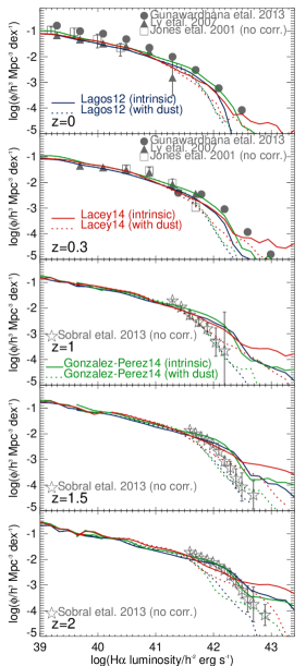
Figure 1: The H$\alpha$ luminosity function, intrinsic and attenuated by dust, at different redshifts (indicated at the lower-left corner of each panel), for the Lagos12, Lacey14 and Gonzalez-Perez14 models, as labelled. Observational estimates of the H$\alpha$ luminosity function from Jones & Bland-Hawthorn (2001), Ly et al. (2007) and Gunawardhana et al. (2013) are shown in the top two panels, and from Sobral et al. (2013) in the bottom three panels using symbols, as labelled. Filled symbols represent observational data that has been corrected for dust extinction (i.e. comparable to the model intrinsic luminosity function), and open symbols represent the observed luminosity function (i.e. comparable to the model extinct luminosity function). Note that we express densities and luminosities in comoving units for both the observations and the models. To transform these units to physical units the reader needs to evaluate $h$ with the value given in $\S$ 2.3.

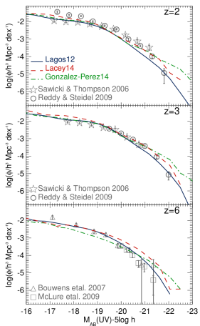
Figure 2: The rest-frame UV(1500Å) luminosity function at $z=2$ (top panel), $z=3$ (middle panel) and $z=6$ (bottom panel) for the Lagos12, Lacey14 and Gonzalez-Perez14 models, as labelled. Symbols represent the observational estimates from Sawicki & Thompson (2006), Bouwens et al. (2007), Reddy & Steidel (2009) and McLure et al. (2009), as labelled. The predictions shown for the models already include the effects of dust extinction and should be compared to the observed luminosity functions without any correction for extinction.The units of density here are as in Fig. 1. However, to convert the magnitudes from the adopted units to $M_{\rm AB}(\rm UV)$ the reader needs to add $5\rm log\,h$ to the quantity in the $x$-axis, where $h$ has the value showed in $\S$ 2.3.

A fair comparison between the observations and the model predictions for the SFR can be made by directly contrasting the observed H$\alpha$ and UV luminosity functions with the predicted ones, which correspond to two of the most popular SFR tracers. Fig. 1 shows the intrinsic H$\alpha$ luminosity function from $z\approx 0$ to $z\approx 1.5$ for the three models and observations. The observations have been separated into those which present the $H\alpha$ luminosity function including a correction for dust attenuation (filled symbols), and those which do not (open symbols). For the three models we show both the intrinsic and dust extincted $H\alpha$ luminosity functions. The intrinsic luminosity functions predicted by the models should be compared to the filled symbols.

The three models have predictions in reasonable agreement with the observations, within the errorbars. At $z=0$ and $z=0.3$, the models predict $H\alpha$ luminosity functions in broad agreement with the observations. At $z=1$, $z=1.5$ and $z=2$ we only show direct observations of the H$\alpha$ luminosity function from Sobral et al. (2013), who present the largest galaxy samples to date, greatly exceeding the number of galaxies and observed sky area from previous works (i.e. $14,011$ emitters in $2.2\,\rm deg^{2}$). These observations are directly comparable to the model predictions that include dust. The three models are consistent with the $z\approx 1$ observations, but are below the observations at $z\approx 1.5$ and $z\approx 2$ at the faint-end by a factor of $\approx 2-3$. This may be due either to a low number of highly star-forming galaxies in the models or to the dust extinction modelling. The former would change the intrinsic H$\alpha$ luminosity function, while the latter would affect only the extincted H$\alpha$ emission. We expect both to contribute to some extent. Differences between the three models in Fig. 1 are mainly seen at the bright-end where the errorbars on the observations are the largest. In general, our dust model predicts that dust attenuation is luminosity dependent, which is a natural consequence of the different gas metallicities in our model galaxies. The faint-end is expected to be only slightly affected by dust, but bright $H\alpha$ galaxies can be highly attenuated by dust. However, the predicted extinctions for $z\gtrsim 1$ are typically smaller than that assumed in observations ($A_{\rm H\alpha}=1$ mag). The Lacey14 model predicts higher number densities of luminous H$\alpha$ galaxies, with intrinsic $L_{\rm H\alpha}>5\times 10^{42}\,h^{-2}\,\rm erg\,s^{-1}$, than the other two models. This is due the predominance of starbursts at these high luminosities and the top-heavy IMF adopted by Lacey14 in bursts. Note that the three models predict that the normalisation and break of the H$\alpha$ luminosity function increase with increasing redshift between $z=0$ and $z=1$, while at $z>1$, the evolution is mainly in the number density of bright galaxies. This overall evolution agrees well with that observed.

At high redshifts, a popular way of studying SF in galaxies is to use the rest-frame FUV emission as a tracer. We compare the predicted rest-frame FUV luminosity function in the three flavours of GALFORM to observations from $z=2$ to $z=6$ in Fig. 2. The observed luminosity function corresponds to the rest-frame $1500$ Å luminosity, without any attempt to correct for dust extinction. This is directly comparable to the model predictions for the rest-frame $1500$ Å luminosity, after dust has been included in the model (lines in Fig. 2). The predictions from the three flavours of GALFORM agree well with the observations, even up to $z=6$. This is partially due to the assumed duration of starbursts. Lacey et al. (2011) show that very short starbursts, such as the ones assumed in Bower et al. (2006), result in the bright-end of the UV luminosity function being largely over predicted. Longer starbursts allow the model to have more dusty starbursts and reproduce the break in the UV LF. The duration of the bursts is of about few $100$ Myr, and therefore in better agreement with the latest estimates of the duration from observational data (Swinbank & et al., 2013).

3.1.2 The cosmic density of SFR

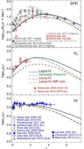
Figure 3: Top panel: Evolution of the global density of the SFR in units of $M_{\odot}\,{\rm yr}^{-1}\,h^{2}\,{\rm Mpc}^{-3}$ for the Lagos12, Lacey14 and Gonzalez-Perez14 models, as labelled. For the Lacey14 model we also show the scaled $\rho_{\rm SFR}$ that would be inferred if a Kennicutt IMF was adopted as universal (dotted line; see text). The grey squares and triangles correspond to the observational estimates of $\rho_{\rm SFR}$ from Sobral et al. (2013) and Gunawardhana et al. (2013), respectively, using H$\alpha$, grey circles to the estimates of Karim et al. (2011), using radio stacking, inverted triangles and filled squares to estimates using the 1500Å emission corrected for dust extinction from Cucciati et al. (2012) and Oesch et al. (2012), respectively, and stars to the estimates of Burgarella et al. (2013) using FUV and FIR. For Sobral et al. we also show their reported $\rho_{\rm SFR}$ integrated only over the range where they have measurements (without extrapolation; circles with inner crosses), and the latter without the dust correction (squares with inner crosses). Middle panel: Evolution of the global density of H₂, in units of the critical density, for the same models. Symbols show the $z\approx 0$ estimate of $\rho_{\rm H_{2}}$ from Keres et al. (2003) using the $\rm CO(1-0)$ luminosity function (filled triangle) and inferences at higher redshifts from Berta et al. (2013) using the molecular masses inferred from the ratio between the UV to the IR emission (open stars). Bottom panel: Evolution of the global density of HI, in units of the critical density, for the three models of the top panel. Observations of $\rho_{\rm HI}$ from Zwaan et al. (2005), Martin et al. (2010) and Freudling et al. (2011) using 21 cm emission, Lah et al. (2007), Delhaize et al. (2013) and Rhee et al. (2013) from spectral stacking, Chang et al. (2010) and Masui et al. (2013) from intensity mapping, and Péroux et al. (2003), Rao et al. (2006), Noterdaeme et al. (2012) and Zafar et al. (2013) from DLAs, are also shown using symbols, as labelled.

We are interested in connecting the evolution of the gas content of galaxies with that of the SFR. With this in mind, we show in Fig. 3 the evolution of the global density of SFR, HI and H₂ for the Lagos12, Lacey14 and Gonzalez-Perez14 models. In the case of the SFR, the observational estimates have been corrected to our choice of IMF (Kennicutt, 1983) (see Appendix A for the conversions). Note that we express the SFR density in comoving units as in Fig. 1. The predictions of the three models are in reasonable agreement with the observational estimates at $z<0.3$ and at $z>2$, within the uncertainties, but significantly lower than the observational estimates in the redshift range $0.3<z<2$. The comparison between the model predictions and the observed density of SFR needs to be undertaken carefully as there are many systematic uncertainties which are not taken into account in the errorbars of the observations. One example is the dust absorption correction applied when ultraviolet bands or emission lines are used to trace SFR (e.g. Hopkins & Beacom 2006). Typically, empirical dust corrections calibrated in the local Universe are extrapolated to high-redshifts (e.g. Calzetti et al. 2007). Another source of uncertainty is related to the extrapolation needed to correct the observed SFR density to account for faint galaxies that are not detected. These two factors drive most of the dispersion observed in Fig. 3 between the different estimates.

To help illustrate the impact of the extrapolation to fainter luminosities and the dust correction, we show in the top panel of Fig. 3 the SFR density from Sobral et al. (2013) which includes both the dust correction and the extrapolation to faint galaxies (squares), the SFR density with the dust correction but integrated only over the range covered by the measurements (circles with inner crosses) and the latter but without the dust correction (squares with inner crosses). The overall effect of the dust correction is at most of $\approx 0.4$ dex and of the extrapolation can be an increase of up to $\approx 0.6$ dex. If the true slope of the H$\alpha$ LF is shallower and/or the dust correction is less dramatic than assumed in the observations the inferred $\rho_{\rm SFR}$ would easily move down closer to our predictions. Recently, Utomo et al. (2014) show evidence that the dust corrections applied in most of the observations shown in the top panel of Fig. 3 are overestimated, leading to an overestimation of the SFRs. Other systematics are hidden in the adopted IMF. Although we scale the inferred observations to our adopted IMF, this conversion is valid only in the case of a simple SF history, for instance a constant SFR, and a constant metallicity, at a certain stellar population age. This is not the case for our simulated galaxies that undergo starbursts and gas accretion which can change the available gas content at any time (Mitchell et al., 2013). Otí-Floranes & Mas-Hesse (2010) argue that the systematic uncertainty due to the IMF choice can be up to a factor of $\approx 4$. Wilkins et al. (2012) show that the ratio between the SFR and the FUV luminosity is correlated with SFR, and that systematic errors relating to adopting a universal ratio can be a factor of $\approx 1.5$ or more. A good example of the uncertainties in the observationally inferred $\rho_{\rm SFR}$ is the fact that the three models predict a H$\alpha$ luminosity function at $z\leq 1$ in broad agreement with the observations (see Fig. 1), but a $\rho_{\rm SFR}$ that is a factor of $\approx 2-4$ lower than the H$\alpha$ inferred $\rho_{\rm SFR}$. Thus, we consider the SFR density inferred from observations as a rough indicator of the SF activity as opposed to a stringent constrain to our model predictions. The fact that the three models have $\rho_{\rm SFR}$ at $z\approx 1$ below the observations is not currently of great concern for two reasons: (i) given the difficulty of quantifying the effect of systematic biases on the observationally inferred $\rho_{\rm SFR}$, and (ii) because the predicted H$\alpha$ and UV luminosity functions are in reasonable agreement with observations.

Overall, the three models predict $\rho_{\rm SFR}$ of a similar shape and normalisation. However, in the detail, we can distinguish two differences that are worth exploring: (i) the Lacey14 model predicts a lower peak of $\rho_{\rm SFR}$ compared to the other two models, and (ii) at $z>6$, there is an offset of a factor of $2-3$ between $\rho_{\rm SFR}$ predicted by the Lagos12 model and the other two models. Feature (i) is due to the adopted top-heavy IMF in starbursts in the Lacey14 model, which results in lower SFRs to drive the same level of FUV, IR and emission line fluxes compared to the choice of a Kennicutt IMF. In fact, we can calculate the difference between the two different IMFs in the flux predicted for the different SFR tracers (see Appendix A). We can scale the contribution from starbursts up by $1.8$ to account for the different IMF; this SFR density would roughly correspond to the inferred one if a Kennicutt IMF was adopted as universal and UV emission was used as a tracer of SF. This is shown by the dotted line in the top panel of Fig. 3. This scaling accounts for most of the difference between the Lacey14 and the other two models that adopt a universal Kennicutt IMF. Feature (ii) is due to the different cosmologies adopted in the Lagos12 (WMAP1) and the other two models (WMAP7). The WMAP7 cosmology has a lower $\sigma_{8}$, which delays the collapse of the first structures, giving rise to the first galaxies at lower redshifts compared to the WMAP1 universe (see Gonzalez-Perez et al. 2013 and Guo et al. 2013 for an analysis of the effect of these cosmologies on galaxy properties). Note that the difference in $\Omega_{\rm m}$ reported by WMAP1 and WMAP7 is irrelevant at these high redshifts as $\Omega_{\rm m}\approx 1$.

3.1.3 The cosmic densities of HI and H₂

The middle and bottom panels of Fig. 3 shows that the atomic and molecular gas densities are predicted to have very different evolution in the three GALFORM models. Note that we have converted all of the observations to our adopted cosmology ($\S$ 2.3). The predicted atomic gas density displays very little evolution at $z\lesssim 2.5$. At higher redshifts, $\rho_{\rm HI}$ slowly decreases with increasing redshift. This behaviour is common in the three models. Quantitatively, $\rho_{\rm HI}$ decreases by only $\approx 11$% between $z=0$ and $z=2.5$ in the three models, while between $z=2.5$ and $z=6$ it decreases by $68$% in the Lagos12 model, $82$% in the Gonzalez-Perez14 model and $80$% in the Lacey14 model. At $z\lesssim 3$, the predicted evolution of the three models agrees well with observations of $\rho_{\rm HI}$ that come either from direct HI detections at $z\approx 0-0.2$ or inferences from spectral stacking, intensity mapping and damped-Ly$\alpha$ systems (DLAs) at $z\gtrsim 0.2$. At $z>3$, the predictions for $\rho_{\rm HI}$ from the three models systematically deviate from the observed $\rho_{\rm HI}$. One reason for this is that we only model neutral gas inside galaxies, i.e. in the ISM, and we do not attempt to estimate the neutral fraction of the gas outside galaxies (i.e. in the IGM). This argument is supported by the results of hydrodynamical simulations which explicitly follow the neutral fraction in different environments. For instance, van de Voort et al. (2012) and Davé et al. (2013) show that the neutral content of the universe in their simulations is dominated by gas outside galaxies at $z\gtrsim 3$.

The weak evolution of $\rho_{\rm HI}$ shown in Fig. 3 contrasts with the evolution of the molecular hydrogen global density, $\rho_{\rm H_{2}}$, which shows a steep increase between $z=0$ and $z=3$ followed by a slow decrease as redshift increases in the three models. Quantitatively, $\rho_{\rm H_{2}}$ increases by a factor $\approx 7$ between $z=0$ and $z=3$ in three models, followed by a decline of a factor of $\approx 3$ for the Lagos12 and Lacey14 models, and of $\approx 5$ for the Gonzalez-Perez14 model between $z=3$ and $z=6$. At $z=0$, the Lagos12 and the Gonzalez-Perez14 models predict a density of H₂ that is in good agreement with the inference of Keres et al. (2003), while the Lacey14 model predicts a H₂ density that is only marginally consistent with the observations. In Appendix B we show the predicted H₂ mass function in the three models compared to observations of Keres et al. and show that this tension between the Lacey14 model and the observationally inferred $\rho_{\rm H_{2}}$ rises from the lower number density of galaxies at the knee of the mass function. We warn the reader, however, that the sample of Keres et al. is not a blind CO survey and also makes use of a constant conversion factor between CO and H₂. Therefore it is unclear how much of this tension is real. (see Lagos et al. 2012 for an illustration of how the CO-H₂ ratio can vary.)

We have also included in the middle panel of Fig. 3 recent inferences of $\rho_{\rm H_{2}}$ from Berta et al. (2013). Berta et al. use the SFR attenuation (the ratio between the emission from the UV and from the mid-IR) to convert to molecular gas content using the empirical relation of Nordon et al. (2013). The two sets of symbols correspond to integrating the inferred H₂ mass function in the range derived by the observed SFRs and integrating down to H₂ masses of $10^{7}\,M_{\odot}$, which requires extrapolation of the inferred H₂ mass function. These two sets of data serve as an indication of the uncertainties in $\rho_{\rm H_{2}}$, although no systematic effects are included in the errorbars. The Lagos12 and Gonzalez-Perez14 models are broadly consistent with the Berta et al. inference, while the Lacey14 model lies below. In $\S$ 4.2, we describe how the physical mechanisms included in the models interplay to drive the evolution of the three quantities shown in Fig. 3.

The Lagos12, Lacey14 and Gonzalez-Perez14 models predict interesting differences, that can be tested in the future. However, with current observations of galaxies, we cannot distinguish between the models. Given that the Lagos12 model has been extensively explored in terms of the gas abundance of galaxies (see for instance Geach et al. 2011 for the evolution of the molecular gas fractions, Lagos et al. 2012 for the evolution of the CO-FIR luminosity relation and luminosity functions, and Kim et al. 2013 for an analysis of the HI mass function and clustering), we use this model in the next sections to explore the contribution from star-forming galaxies to the densities of SFR, HI and H₂. In $\S$ 4.3, we explore how robust these predictions are by comparing with the Lacey14 and Gonzalez-Perez14 models. However, we remark that the other two models give similar results to the Lagos12 model in the comparisons presented in $\S$ 3.2 and 3.3.

3.2 The evolution of normal star-forming galaxies

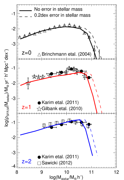
Figure 4: Star formation rate density as a function of stellar mass for three different redshifts, as labelled, for the Lagos12 model. Solid lines show the model predictions and dashed lines show, for reference, the effect of including an error of $0.2$ dex in the stellar mass estimate (see Mitchell et al. 2013 for a complete discussion on the uncertainties in stellar mass estimates). We show the observational results from Brinchmann et al. (2004) at $z\approx 0.2$, Gilbank et al. (2010) at $z\approx 1$, Karim et al. (2011) at $z\approx 1$ and $z\approx 2$, and Sawicki (2012) at $z\approx 2$. Note that we express densities and masses in comoving units for both the observations and the models. To transform these units to physical units the reader needs to divide the mass by the value of $h$ given in $\S$ 2.3, and multiply the density by the $h$ value squared.

An important test of the model is the observed relation between the SFR density at fixed stellar mass, $\rho_{\rm SFR,M}$, and stellar mass at a given redshift. Several works have analysed this relation and concluded that it is very difficult for current semi-analytic models and simulations of galaxy formation to predict the right trends. The argument is that this relation is very sensitive to feedback mechanisms and how inflow and outflow compensate to each other (e.g. Dutton et al. 2010; Fontanot et al. 2009; Lagos et al. 2011b; Davé et al. 2011; Weinmann et al. 2012).

Observationally, $\rho_{\rm SFR,M}$ is constructed using galaxies with detected SFRs (i.e. above a sensitivity limit in SFR). These galaxies are refer to as ‘star-forming’, and lie on a tight relationship between the stellar mass and the SFR (Schiminovich et al. 2007; Noeske et al. 2007; Elbaz et al. 2007), with outliers typically being starbursts, which have disturbed dynamics (e.g. Wuyts et al. 2011). However, in the model we include all the galaxies in a given stellar mass bin, even if they have low SFRs, to calculate $\rho_{\rm SFR,M}$ given that passive galaxies, which lie below the sequence of star-forming galaxies, contribute very little to the global SFR (Lagos et al. 2011b). We show the $\rho_{\rm SFR,M}$-stellar mass distribution function at three different redshifts in Fig. 4. Observational data have been scaled to our choice of IMF using the scalings described in Appendix A.

There are three interesting aspects of Fig. 4. First, the Lagos12 model predicts that the highest contribution to $\rho_{\rm SFR}$ comes from relatively massive galaxies and that this peak mass, $M_{\rm s}$, increases slightly with increasing redshift, from $M_{\rm s}\approx 2\times 10^{10}\,M_{\odot}\,h^{-1}$ at $z=0$ to $M_{\rm s}\approx 4\times 10^{10}\,M_{\odot}\,h^{-1}$ at $z=2$. The stellar mass corresponding to the peak of $\rho_{\rm SFR,M}$ is also consistent with the recent observational inferences of the $\rho_{\rm SFR,M}$ distribution function by Sobral et al. (2013). In the model, this increase of a factor of $2$ is driven by the higher frequency of bright starbursts at high redshifts, which are also more frequent in massive galaxies, $M_{\rm stellar}>10^{10}\,M_{\odot}\,h^{-1}$ (see Lagos et al. 2011b). Secondly, the drop in the contribution to $\rho_{\rm SFR}$ from galaxies with stellar masses above $M_{\rm s}$ becomes steeper with increasing redshift, which is related to the low number density of galaxies more massive than $M_{\rm s}$ at high-redshift; i.e. the break in the stellar mass function becomes smaller than $M_{\rm s}$ at $z\gtrsim 2$ (Behroozi et al., 2013). Finally, the slope of the relation between $\rho_{\rm SFR,M}$ and $M_{\rm stellar}$ below $M_{\rm s}$ is very weakly dependent on redshift, but the normalisation increases with increasing redshift. Below $M_{\rm s}$, most of the galaxies lie on the SFR-stellar mass sequence of star-forming galaxies. Thus the slope of the $\rho_{\rm SFR,M}$-$M_{\rm stellar}$ is set by the slope of the SFR-stellar mass relation. Lagos et al. (2011b) show that this slope is sensitive to how quickly the gas that is expelled from the galaxy by stellar feedback reincorporates into the halo and becomes available for further cooling. Lagos et al. show that the model predicts a slope close to the observed one if this reincorporation timescale is short (i.e. of the order of a few halo dynamical timescales). The observations do not have yet the volumes and sensitivity limits needed to probe these three features, but with the current observations and the comparison with the model predictions we can conclusively say that the normalisation of the $\rho_{\rm SFR,M}$-$M_{\rm stellar}$ relation increases with increasing redshift, and that there is a stellar mass where the relation peaks.

Overall the model predicts a $\rho_{\rm SFR,M}$-$M_{\rm stellar}$ relation in reasonable agreement with the observations. The differences between the predictions of the model and the observations are in the range $0.1-0.3$ dex. When integrating over stellar mass to give $\rho_{\rm SFR}$, as presented in Fig. 3, the differences add up to make the large deviations shown in Fig. 3. Note that at $z=2$, the Lagos12 model predicts a lower $M_{\rm s}$ than observed. This could be due to the fact that we are not including any error source for the stellar mass and SFRs in the model (see Marchesini et al. 2009; Mitchell et al. 2013). We show in Fig. 4 the convolution of our predicted stellar masses with a Gaussian of width $0.2$ dex to illustrate the effect of this uncertainty on the predictions. Once uncertainties are taken into account, the predicted $M_{\rm s}$ agrees better with observations.

3.3 The frequency of highly star-forming galaxies

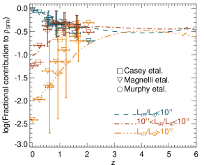
Figure 5: Fractional contribution of galaxies with different IR luminosities, as labelled in units of $L_{\odot}$, to the global density of SFR for the Lagos12 model, as a function of redshift. The observational estimates of Murphy et al. (2011), Casey et al. (2012) and Magnelli et al. (2013) are shown as symbols. For clarity, errorbars in the $y$-axis for the observations are shown only for Murphy et al.

A commonly used tracer for SF is the IR luminosity, which approximates to the total luminosity emitted by interstellar dust, which, in media that are optically thick to UV radiation, is expected to correlate closely with the SFR. Infrared galaxy surveys have changed our view of the contribution from IR luminous galaxies to the IR background, or the global SFR density (e.g. Le Floc’h et al. 2005). From these surveys it is now clear that the contribution from the most luminous IR galaxies to $\rho_{\rm SFR}$ increases dramatically with increasing redshift. New mid- and far-IR surveys have allowed the characterisation of the contribution to the IR background and $\rho_{\rm SFR}$ from galaxies with IR luminosities down to $L_{\rm IR}\approx 10^{10}L_{\odot}$ between $z=0$ and $z\approx 1.5$. These observations allowed the quantification of how more frequent bright IR galaxies are at high-redshift compared to the local Universe.

We compare in Fig. 5 the predicted fractional contributions to $\rho_{\rm SFR}$ from galaxies with different IR luminosities in the Lagos12 model to recent observational estimates from Murphy et al. (2011), which combine measurements at $24\mu$m and $70\mu$m, Casey et al. (2012) using Herschel-SPIRE $250\mu$m, $350\mu$m and $500\mu$m bands and Magnelli et al. (2013), which use the Herschel-PACS $70\mu$m, $100\mu$m and $160\mu$m bands. The use of several IR bands ensures the detection of the peak of the IR spectral energy distribution and an accurate estimate of the total IR luminosity. Our model predicts that at $z\gtrsim 3$, the three bins of IR luminosity contribute similarly to $\rho_{\rm SFR}$. At lower redshifts the situation is very different. At $z<1$, $\rho_{\rm SFR}$ is dominated by galaxies with $L_{\rm IR}<10^{11}L_{\odot}$, while between $1<z<2$, $\rho_{\rm SFR}$ is dominated by galaxies with $L_{\rm IR}>10^{11}L_{\odot}$. These bright IR galaxies in the Lagos12 model correspond to a combination of normal star-forming galaxies and starbursts. Note that the brightest IR galaxies make a negligible contribution to $\rho_{\rm SFR}$ at $z<1.5$, but their contribution increases up to $34$% of the total at $z\approx 3$. We find that the Lagos12 model predicts fractional contributions to $\rho_{\rm SFR}$ that are in good agreement with the observations. Although there are systematic differences in the inferred contribution from the brightest IR galaxies to $\rho_{\rm SFR}$ between the observational samples, they are still consistent with each other within the errors. Magnelli et al. (2013) argue that one possible driver of such systematics is the spectroscopic redshift incompleteness, which is different for each sample.

4 The contribution from star-forming galaxies to the densities of atomic and molecular gas

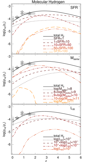
Figure 6: Global density of atomic (left panels) and molecular hydrogen (right panels) in units of the critical density, as a function of redshift for the Lagos12 model. The contributions from galaxies with different SFRs (top panels), stellar masses (middle panels) and IR luminosities (bottom panels) are shown by different lines, as labelled in each panel. The SFRs in the top panels are in units of $M_{\odot}\,\rm yr^{-1}$, stellar masses in the middle panels are in $M_{\odot}$ and IR luminosities in the bottom panels are in $L_{\odot}$. Observational estimates are as in Fig. 3.

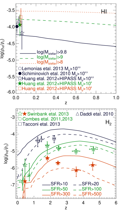
Figure 7: Top panel: Global density atomic hydrogen in units of the critical density, as a function of redshift for massive galaxies in the Lagos12 model, as labelled. Stellar masses are given in units of $M_{\odot}$. We also plot the estimate of $\rho_{\rm HI}$ for galaxies with $M_{\rm stellar}>10^{9.9}\,M_{\odot}$ from Schiminovich et al. (2010) and Lemonias et al. (2013), for three stellar mass limits by combining the HI mass function of Zwaan et al. (2005) and the HI-stellar mass relation of Huang et al. (2012). The stellar mass limit in Schiminovich et al. and Lemonias et al. has been corrected from their assumed Chabrier IMF to our adopted Kennicutt IMF. The scatter of the inferred values in the latter estimates is large due to the scatter in the HI-stellar mass relation. We thus show three bins of stellar mass for model galaxies that should be comparable to the three bins with available observational data. Bottom panel: Global density of molecular hydrogen in units of the critical density, as a function of redshift for the most highly star-forming galaxies in the Lagos12 model, as labelled. The SFRs are in units of $M_{\odot}\,\rm yr^{-1}$. We compare our predicted $\rho_{\rm H_{2},SFR}$ with observational inferences from Swinbank & et al. (2013), which include their sub-millimeter galaxy sample and previous samples from Daddi et al. (2010), Tacconi et al. (2013) and Combes et al. (2011,2013). The samples of sub-millimeter galaxies from Swinbank et al. is divided into two, those with fluxes at $850\mu$m $>1$ mJy, which roughly corresponds to SFR$\gtrsim 100\,M_{\odot}\rm\,yr^{-1}$, and those with fluxes $>4.2$ mJy, which roughly corresponds to SFR$\gtrsim 300\,M_{\odot}\rm\,yr^{-1}$. The samples of Tacconi et al. and Daddi et al. correspond to star-forming galaxies in the main sequence of star formation, which have SFR$\gtrsim 20\,M_{\odot}\rm\,yr^{-1}$, while the sample of Combes et al. corresponds to ultra luminous IR galaxies, which roughly have SFR$\gtrsim 100\,M_{\odot}\rm\,yr^{-1}$.

The main goal of this paper is to explore the contribution from galaxies with different properties to the overall HI and H₂ content of the universe. From this we gain an insight into how far observations currently are from tracing the bulk of the neutral gas in galaxies in the universe. In this section we start by describing the contribution from star-forming galaxies to $\rho_{\rm HI}$ and $\rho_{\rm H_{2}}$ and then we analyse the physical drivers behind the trends found in $\S$ 4.2. In $\S$ 4.3 we investigate how robust these trends are by comparing the three GALFORM models (described in $\S$ 2). We will refer to the HI and H₂ densities of galaxies selected by their SFR as $\rho_{\rm HI,SFR}$ and $\rho_{\rm H_{2},SFR}$, respectively, and by stellar mass as $\rho_{\rm HI,m}$ and $\rho_{\rm H_{2},m}$, respectively. We remind the reader that both gas components correspond exclusively to gas in galaxies, and that any neutral gas outside galaxies is not accounted for. As in Fig. 3, we have converted all of the observations to our adopted cosmology ($\S$ 2.3).

4.1 Stellar mass and SFR dependence of $\rho_{\rm HI}$ and $\rho_{\rm H_{2}}$

We first discuss the HI content of galaxies, then their H₂ content and finish with what we expect for galaxies with different IR luminosities.

HI in galaxies. The top left-hand panel of Fig. 6 shows the evolution of the contribution from galaxies with different SFRs to $\rho_{\rm HI}$ for the Lagos12 model. Most of the galaxies that account for the HI content of the universe have modest SFRs, SFR$<1\,M_{\odot}\rm\,yr^{-1}$, at any time. This galaxy population alone makes up $\approx 80$% of $\rho_{\rm HI}$ at $z=0$ and $\approx 94$% at $z=6$. The remaining HI is found mainly in galaxies with SFRs in the range $1<\rm SFR$$/M_{\odot}\,\rm yr^{-1}<10$. Galaxies with high SFRs, $\rm SFR$$>10\,M_{\odot}\,\rm yr^{-1}$, only contribute $\approx 0.7$% to $\rho_{\rm HI}$ at $z=0$ and reach a maximum contribution of $\approx 2.3$% at $z=3$. The form of $\rho_{\rm HI,SFR}$ vs. redshift for galaxies with low and high SFRs is very different. The former monotonically decreases with look-back time, while the latter have $\rho_{\rm HI,SFR}$ slowly increasing from $z=0$ to $z\approx 2-3$, followed by a gentle decline.

The middle left-hand panel of Fig. 6 shows the evolution of the contribution from galaxies of different stellar masses to $\rho_{\rm HI}$ for the Lagos12 model. All galaxies, passive and star-forming, have been included in the figure. Model galaxies with $M_{\rm stellar}<10^{9}\,M_{\odot}$ dominate the HI content of the universe at $z\lesssim 1$, while at $z\gtrsim 1$ most of the HI is locked up in galaxies with $M_{\rm stellar}<10^{8}\,M_{\odot}$. Our model predicts that galaxies with $M_{\rm stellar}>10^{10}\,M_{\odot}$ build up $\approx 14$% of the HI content of the universe at $z=0$. Schiminovich et al. (2010) and Lemonias et al. (2013) estimated $\rho_{\rm HI,m}$ in the observed galaxies of the GALEX Arecibo SDSS Survey (GASS) survey, which is a stellar mass selected catalogue of local Universe galaxies (see top panel of Fig. 7). For our adopted IMF, galaxies in the GASS sample have $M_{\rm stellar}>8.9\times 10^{9}\,M_{\odot}$. We calculate $\rho_{\rm HI,m}$ of model galaxies selected using the same stellar mass cut at $z=0$ and find that our prediction is a factor $\approx 0.1-0.2$ dex lower than the observational inference. The exact factor depends on the treatment of the non-detections in the observations. This difference could be partially explained as being driven by cosmic variance; our simulated volume is relatively small, and we lack the very gas-rich galaxies with HI masses comparable to the most gas-rich galaxies included in Schiminovich et al. and Lemonias et al. to infer $\rho_{\rm HI,m}$ of massive galaxies. Another source of discrepancy is related to the crude treatment of stripping of HI gas in galaxy groups and clusters. In our model, when galaxies become satellites, they instantaneously lose their hot gas reservoir (i.e. strangulation of hot gas), transferring it to the central halo while slowly consuming ther remaining gas in the ISM. A more accurate treatment may be needed to explain the neutral gas content of galaxies in groups and clusters (Lagos, Davis et al. in preparation).

With the aim of making a more quantitative comparison to lower stellar mass bins, we calculate $\rho_{\rm HI,m}$ for galaxies with $M_{\rm stellar}>10^{8}\,M_{\odot}$, $M_{\rm stellar}>10^{9}\,M_{\odot}$ and $M_{\rm stellar}>8.9\times 10^{9}\,M_{\odot}$ by combining the observed HI mass function of Zwaan et al. (2005) with the HI-stellar mass relation found by Huang et al. (2012) for the ALFALFA sample, corrected to a Kennicutt IMF. The Lagos12 model predictions show good agreement with these observationally inferred $\rho_{\rm HI,m}$ in the three mass bins. The scatter of the observationally inferred $\rho_{\rm HI,m}$ is rather large due to the scatter in the HI-stellar mass relation.

Compared to previous theoretical estimates, we find that our predictions for $\rho_{\rm HI,m}$ agree well with the predicted trends in Davé et al. (2013). Davé et al. find that most of HI in the universe, which in their case corresponds to both HI in galaxies and in the intergalactic medium, is locked up in galaxies with stellar masses $\lesssim 10^{8}\,M_{\odot}$ at $z>1.5$. At $z<1.5$, Davé et al. find that galaxies with stellar masses in the range $10^{8}-10^{9}\,M_{\odot}$ increase their contribution to $\rho_{\rm HI}$ to similar values as the lower stellar mass galaxies. These trends are similar to the ones we find for the Lagos12 model. Popping et al. (2013a) include in a semi-analytic model of galaxy formation similar SF laws to those that were developed in Lagos et al. (2011b) and found that the HI density is dominated by galaxies with $M_{\rm stellar}<10^{7},M_{\odot}$, which is even lower than in our case. These predictions from Popping et al. may be in slight tension with the observationally inferred contribution from galaxies with $M_{\rm stellar}>10^{8},M_{\odot}$ shown in Fig. 6, which can account for $\approx 70$% of the observed HI mass density at $z=0$, albeit with large errorbars.

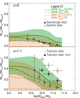
Figure 8: Molecular gas fraction, defined as $f_{\rm gas}=M_{\rm mol}/(M_{\rm mol}+M_{\rm stellar})$, where $M_{\rm mol}$ includes hydrogen and helium, as a function of stellar mass, at $z=0$ (top panel) and $z=1.1$ (bottom panel) for the Lagos12 model. Central and satellite galaxies are shown separately, each for two selections in molecular gas fraction, $f_{\rm gas}>0$ and $f_{\rm gas}>0.01$. The aim of this is to show how sensitive the predicted trends are to selection effects that are typically present in observations. Lines show the median of the relations, and the shaded regions represent the $10$ and $90$ percentiles and are shown only for the case of centrals and satellites with $f_{\rm gas}>0.01$. At $z\approx 0$, filled circles show the observationally inferred trend from the carbon monoxide survey of Saintonge et al. (2011), at $z\approx 0$ and $z=1.1$ stars show H₂ inferred masses from the dust measurements of Santini et al. (2013) using Herschel, and the $z=1.1$ observations of Tacconi et al. (2013) of carbon monoxide in normal star-forming galaxies with and without the incompleteness correction are shown as filled and empty squares, respectively. Note that we express masses in physical units. For these we corrected all of the observations to our adopted cosmology ($\S$ 2.3).

H₂ in galaxies. The behaviour of star-forming galaxies in the $\rho_{\rm H_{2}}$-z plane, shown in the top and middle right-hand panels of Fig. 6, contrasts with that in the $\rho_{\rm HI}$-z plane. Galaxies with SFR$<1\,M_{\odot}\rm\,yr^{-1}$ represent $\approx 35$% of the H₂ at $z=0$ and only $\approx 15$% at $z=3$. Galaxies with $1<\rm SFR$$/M_{\odot}\,\rm yr^{-1}<10$ contribute $\approx 56$% of the H₂ at $z=0$, and their contribution also decreases with increasing redshift, yielding $\approx 40$% at $z=2$. One of the most interesting predictions of the top right-hand panel of Fig. 6 is that galaxies with $10<\rm SFR$$/M_{\odot}\,\rm yr^{-1}<50$ contain a large fraction of the $H_{2}$ of the universe at high-redshift, reaching a maximum contribution of $\approx 40$% at $z=2$. Highly star-forming galaxies are also more important in H₂ than HI, reaching a maximum contribution of $\approx 9$% in the redshift range $z\approx 3.5-4.5$. As in $\rho_{\rm HI}$, the functional form of $\rho_{\rm H_{2},SFR}$ of highly star-forming galaxies is very different from that of galaxies with modest SFRs. Galaxies with SFR$<10\,M_{\odot}\rm\,yr^{-1}$ give a $\rho_{\rm H_{2},SFR}$ slowly increasing with redshift up to $\approx 3.5$, followed by a very slow decline at higher redshifts, while galaxies with SFR$>10\,M_{\odot}\rm\,yr^{-1}$ show $\rho_{\rm H_{2},SFR}$ increasing by more than a factor $\approx 30$ between $z=0$ and $z\approx 2$.

Observational estimates of $\rho_{\rm H_{2},SFR}$ are very scarce and subject to strong systematics, such as the choice of CO-H₂ conversion factor, the dust-to-gas mass ratio and the characterisation of the selection function. Even though these uncertainties limit current possibilities to derive the quantities above, it is possible to use available CO surveys of highly star-forming galaxies to infer $\rho_{\rm H_{2},SFR}$ to within a factor of $\approx 2-3$. Swinbank & et al. (2013) infer $\rho_{\rm H_{2},SFR}$ for galaxies with SFR$\gtrsim 30\,M_{\odot}\rm\,yr^{-1}$. Swinbank et al. analyse the H₂ abundance of sub-millimeter galaxies, together with three other samples of galaxies with SFRs $\gtrsim 100\,M_{\odot}\rm\,yr^{-1}$ from Combes et al. (2011) and Combes et al. (2013), and with SFRs $\gtrsim 20\,M_{\odot}\rm\,yr^{-1}$ from Daddi et al. (2010) and Tacconi et al. (2013). To calculate $\rho_{\rm H_{2}}$ from the samples of Tacconi et al. and Combes et al. is not straightforward, given the complexity of the selection functions. With this in mind, Swinbank et al. used simulated galaxy catalogues from the Millennium database to select model galaxies using the same observational selection criteria (in H_α or IR luminosity, optical luminosity and stellar mass), which informed the number density of galaxies that resemble the samples of Tacconi et al. and Combes et al.. Swinbank et al. used these number densities to estimate $\rho_{\rm H_{2}}$ from the samples of Tacconi et al. and Combes et al.

Note that the SFR lower limit in the observed samples is approximate and can vary by a factor of $\approx 2$. We compare the estimates of Swinbank et al. with our predicted $\rho_{\rm H_{2},SFR}$ for these highly star-forming galaxies in the bottom panel of Fig. 7. To illustrate the effect of varying the SFR limits by a factor of $2$, we show in Fig. 7 $\rho_{\rm H_{2},SFR}$ for galaxies with SFR$\gtrsim 50\,M_{\odot}\,\rm yr^{-1}$ and SFR$\gtrsim 100\,M_{\odot}\,\rm yr^{-1}$, which are compared to the inferences of $\rho_{\rm H_{2},SFR}$ by Swinbank et al. for the samples of Combes et al. and their faint sub-millimeter galaxies (SMGs), and with SFR$\gtrsim 300\,M_{\odot}\,\rm yr^{-1}$ and SFR$\gtrsim 500\,M_{\odot}\,\rm yr^{-1}$, which are compared to the sample of Swinbank et al. of bright SMGs. To compare with the estimates presented by Swinbank et al. using the Daddi et al. and Tacconi et al. samples, we show the predicted $\rho_{\rm H_{2},SFR}$ for galaxies with SFR$\gtrsim 10\,M_{\odot}\,\rm yr^{-1}$ and SFR$\gtrsim 20\,M_{\odot}\,\rm yr^{-1}$. Swinbank et al. argue that there are systematic effects in the estimates of the number densities of sources in addition to other systematics effects related to the CO-to-H₂ conversion factor. This implies that the errorbars on the observational data in Fig. 7 are likely to be lower limits to the true uncertainty. Note that the samples of Daddi et al., Tacconi et al. and Combes et al. correspond to observations of CO, while Swinbank et al. used inferred dust masses from their FIR observations to estimate H₂ masses by adopting a dust-to-gas mass ratio. The model predictions are in good agreement with the observations, within the errorbars, over the whole redshift range. Note that the data here gives independent constrains on our model than those provided by Berta et al. and shown in Fig. 3. Galaxies used to calculate $\rho_{\rm H_{2},SFR}$ in the observations, as in our model predictions, are a mixture of merging systems and normal star-forming galaxies (which are referred to in our model as quiescent galaxies), which has been concluded from the measured velocity fields of the CO emission lines in some of the observed galaxies.

The trends between $\rho_{\rm H_{2},m}$ and stellar mass in the middle right-hand panel of Fig. 6 are again very different from those obtained for $\rho_{\rm HI}$. We find that $\rho_{\rm H_{2}}$ is dominated by relatively massive galaxies, $10^{10}\,M_{\odot}<M_{\rm stellar}<10^{11}\,M_{\odot}$, from $z=0$ up to $z\approx 3$. Note that the contribution from these galaxies to $\rho_{\rm H_{2}}$ increases from $42$% at $z=0$ to $52$% at $z=1.5$. At $z\gtrsim 3$, galaxies with lower stellar masses, $10^{8}\,M_{\odot}<M_{\rm stellar}<10^{10}\,M_{\odot}$, dominate the H₂ content. It is also interesting to note that Karim et al. (2011) and Sobral et al. (2013) find that the SFR density is dominated by galaxies with stellar masses in the range $1.4\times 10^{10}\,M_{\odot}<M_{\rm stellar}<10^{11}\,M_{\odot}$, which overlaps with the stellar mass range we find to dominate $\rho_{\rm H_{2}}$. Note that the contribution from galaxies with $M_{\rm stellar}<10^{8}\,M_{\odot}$ is resolved, as higher resolution runs produce the same small contribution agreeing to a factor of better than $5$% (see Appendix C).

In Fig. 8, we compare the relation between the molecular gas fraction and the stellar mass in the model with observations of CO emission lines (Saintonge et al. 2011; Tacconi et al. 2013) and dust masses (Santini et al., 2013). From this figure we can draw two main conclusions. First, our model predicts a strong evolution of the molecular gas fraction that agrees well with the observationally inferred one (see also Geach et al. 2011 for a former comparison), and second, the comparison with observations needs to be done carefully, as the predicted evolution strongly depends on galaxy properties, such as the gas fraction itself, stellar mass or halo mass. Observations other than at $z=0$ are strongly biased towards high molecular gas fractions, and therefore observations at $z=1.1$ should be compared with the evolution predicted for galaxies with molecular gas fractions that are above $1$%. Another interesting aspect is the difference between central and satellite galaxies, which comes mainly from the lack of cooled gas accretion in satellites. Lagos et al. (2011b) show that most of the galaxies in the main sequence of the SFR-$M_{\rm stellar}$ plane correspond to central galaxies in the model, and therefore observed galaxies, which also fall in this main sequence, should be compared to our expectations for centrals.

The dependence on IR luminosity. In the bottom panels of Fig. 6 we show the contribution to the HI and H₂ densities from galaxies with different IR luminosities. This quantity is more easily inferred from observations than the SFR or stellar masses, which, as we discussed in $\S$ 3, are affected by systematic uncertainties that are not accurately constrained. The IR luminosity, on the other hand, is well estimated from photometry in few IR bands (e.g. Elbaz et al. 2010). The trends seen with IR luminosity in Fig. 6 are similar to those obtained for the SFR (top panels of Fig. 6). This is due to the good correlation between the IR luminosity and the SFR predicted by the model. However, the normalisation of the $L_{\rm IR}$-SFR relation is predicted to vary with SFR and redshift, due to the underlying evolution of gas metallicity and the gas density in the ISM of galaxies.

4.2 The physical drivers of the gas content of star-forming galaxies

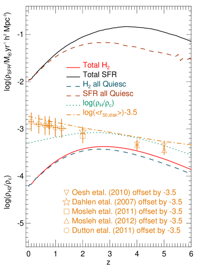
Figure 9: Global density of the SFR in units of $M_{\odot}\,{\rm yr}^{-1}\,h^{2}\,{\rm Mpc}^{-3}$ (black line), and of the molecular hydrogen (red line) in units of the critical density, as a function of redshift for the Lagos12 model. We show the contribution from quiescent star formation (i.e. taking place in the galaxy disk) as dashed lines, the evolution of the neutral hydrogen gas, atomic plus molecular, in the ISM of galaxies in units of $\rho_{\rm c}$ as dotted line and the evolution of the median half-mass radius,$\langle r_{\rm disk}\rangle$, of late-type galaxies with stellar masses in the range $7\times 10^{9}\,M_{\odot}<M_{\rm stellar}<10^{10}\,M_{\odot}$, as dot-dashed line. The latter range is chosen to make it comparable to the observational inferences. The units of $\langle r_{\rm disk}\rangle$ are $\rm kpc$, and $\rm log($$\langle r_{\rm disk}\rangle)$ are plotted offset by $-3.5$ to fit in the figure. We also show the observational estimate of the half-light radius evolution from Dutton et al. (2011) Dahlen et al. (2007), Oesch et al. (2010), Mosleh et al. (2011) and Mosleh et al. (2012) for galaxies with stellar masses $\sim 8.9\times 10^{9}\,M_{\odot}$. Note that the errorbars in the data of Dutton et al. show the $1\sigma$ dispersion around the median of the size-mass relation, while the other observations quote Poisson errors and are therefore not necessarily representative of the true dispersion of the size-mass relation. The units of the observational measurements of $r_{\rm disk}$ are kpc and are shifted by $-3.5$ dex, as are the model predictions. The units for densities are comoving, as in Fig. 3. In the case of the half-light radius, the units are physical and therefore we have scaled the observations to our adopted cosmology ($\S$ 2.3).

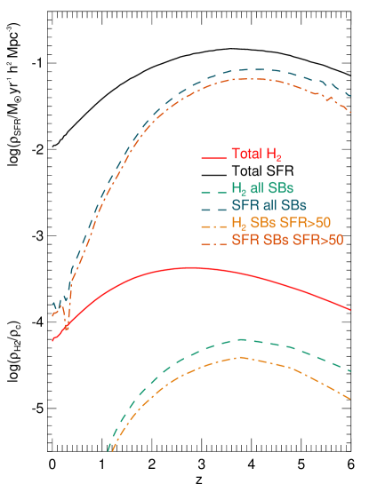
Figure 10: Global density of the SFR in units of $M_{\odot}\,{\rm yr}^{-1}\,h^{2}\,{\rm Mpc}^{-3}$ (black line), and of the molecular hydrogen (red line) in units of the critical density, as a function of redshift for the Lagos12 model. We show the contribution from all starburst galaxies (i.e. those with at least 50% of their global SFR taking place in a starburst) to $\rho_{\rm SFR}$ and $\rho_{\rm H_{2}}$ as dashed lines, and from starburst galaxies with SFR $\geq 50~{}M_{\odot}\,\rm yr^{-1}$ as dot-dashed lines. The units for densities are comoving, as in Fig. 3.

There are three key physical processes that drive the trends with SFR and stellar mass in Fig. 6; (i) the regulation between gas outflows and accretion of gas onto galaxies, (ii) the size evolution of normal star-forming galaxies (i.e. which undergo quiescent SF) and its effect on the gas surface density, and (iii) the frequency of starbursts and its evolution. Below we summarise the main effects each of these physical processes have on $\rho_{\rm SFR}$, $\rho_{\rm HI}$ and $\rho_{\rm H_{2}}$.

Evolution in $\rho_{\rm cold}$. The evolution of the total density of cold gas $\rho_{\rm cold}=\rho_{\rm HI}+\rho_{\rm H_{2}}$ is shown in Fig. 9. Also shown are the evolution of $\rho_{\rm SFR}$ and $\rho_{\rm H_{2}}$ for all galaxies, for all quiescent galaxies, and the median half-mass radius of all galaxies with stellar masses in the range $7\times 10^{9}\,M_{\odot}<M_{\rm stellar}<10^{10}\,M_{\odot}$.

Quiescent SF dominates the SFR in the universe at $z\lesssim 2.8$, and at higher redshift it contributes $\approx 30-50$% to $\rho_{\rm SFR}$. The peak of $\rho_{\rm SFR}$ for quiescent galaxies takes place at lower redshift than for starbursts. The evolution of $\rho_{\rm SFR}$ of quiescent galaxies is very similar to the evolution of $\rho_{\rm H_{2}}$, reassuring our previous statement that starbursts contribute very little to $\rho_{\rm H_{2}}$. The latter closely follows $\rho_{\rm cold}$ at $z\gtrsim 2$. The evolution of $\rho_{\rm cold}$ is driven by the balance between accretion of gas and outflows from galaxies. On average, accretion and outflows in galaxies at a given time self-regulate in a way that the SFR-$M_{\rm stellar}$ relation is characterised by a small dispersion and a power-law index of $\approx 0.8-0.9$ (Lagos et al., 2011b). Small perturbations to this self-regulation phase of galaxy growth drive the slow evolution of $\rho_{\rm cold}$ and of the normalisation of the SFR-$M_{\rm stellar}$ relation of normal star-forming galaxies. In the regime where $\rho_{\rm HI}\gg\rho_{\rm H_{2}}$, which is the case at $z\lesssim 1$, $\rho_{\rm HI}$ follows very closely the evolution of $\rho_{\rm cold}$. At $z\gtrsim 4$, the ratio between $\rho_{\rm H_{2}}$ and $\rho_{\rm HI}$ evolves slowly, and therefore $\rho_{\rm H_{2}}$ and $\rho_{\rm HI}$ decrease with increasing redshift at a similar rate as $\rho_{\rm cold}$ decreases. This can be seen in the evolution of the former two quantities shown in Fig. 3 and of $\rho_{\rm cold}$ shown in Fig. 9. In the intermediate redshift regime, $2<z<4$, $\rho_{\rm H_{2}}\gtrsim\rho_{\rm HI}$, and therefore $\rho_{\rm H_{2}}$ peaks at a similar redshift as $\rho_{\rm cold}$.

At $z<3$, the evolution of $\rho_{\rm H_{2}}$ and $\rho_{\rm SFR}$ of quiescent galaxies is more dramatic than it is for $\rho_{\rm cold}$. This is due to the fact that the ratio $\rho_{\rm H_{2}}/\rho_{\rm HI}$ for quiescent galaxies is strongly evolving due to the change in the surface density of gas plus stars, which change the hydrostatic pressure in the midplane of disks. A factor that strongly affects the evolution of the surface density of gas and stars is the evolution in the sizes of galaxies.

Evolution in size. On average, galaxy sizes increase with time (see Fig. 9). What drives the growth in the sizes of galaxy disks with time is the angular momentum of the accreted gas. As the universe expands, gas that gets to galaxies comes from further out, which means that it brings higher angular momentum compared to gas that was accreted in the past. If the angular momentum loss is small, the newly cooled gas that is accreted settles down at an outer radius, increasing the half-mass radius (see Cole et al. 2000 for a quantitative description of the size evolution of galaxies in GALFORM). We compare the evolution of sizes in the model galaxies with the observed increase reported. Note that in the case of Dahlen et al. (2007), Oesch et al. (2010) and Mosleh et al. (2011,2012) there is no morphological selection and the size evolution is measured for all galaxies, while in the case of Dutton et al. (2011), the reported half-light radius evolution is for late-type galaxies only. In all cases we plot the reported evolution for galaxies with stellar masses $M_{\rm stellar}\sim 8.9\times 10^{9}\,M_{\odot}$. The stellar masses of the observed samples have been scaled from a Chabrier (2003) to a Kennicutt (1983) IMF. In the model we select all late-type galaxies (i.e. bulge-to-total stellar mass ratio $<0.5$) with stellar masses in the range $7\times 10^{9}\,M_{\odot}<M_{\rm stellar}<10^{10}\,M_{\odot}$ and calculate the median half-mass radius of their disks. We find that the growth rate of galaxies agrees well with the observations, although with small discrepancies at higher redshifts towards larger radii. The observed samples at these high-redshifts are very small and encompass all galaxies, late- and early-type, which can bias the size-stellar mass relation toward smaller sizes. In addition, only Poisson errors have been reported which makes it difficult to estimate the significance of the deviations above. At $z>5$ there are only a handful of galaxies with stellar masses in the range we plot and therefore we do not show them in this figure.

The size evolution has an effect on the gas surface density, and therefore on $\rho_{\rm H_{2}}/\rho_{\rm HI}$ and $\rho_{\rm SFR}$. Quantitatively, $\rho_{\rm H_{2}}$ decreases by $\approx-0.9$ dex from $z\approx 2.5$ to $z=0$. In the same redshift range, $\rho_{\rm cold}$ decreases by $\approx-0.3$ dex and the median size of late-type galaxies in the model increases by $0.4$ dex. From combining the evolution in $\rho_{\rm cold}$ and $\langle r_{\rm 50}\rangle$ in the regime where $\Sigma_{\rm cold}\gg\Sigma_{\rm stellar}$, we can derive the expected change in $\rho_{\rm H_{2}}$ to be $-1.2$ dex. This number is an upper limit on the magnitude of the variations in $\rho_{\rm H_{2}}$ between $\approx 2.5$ and $z=0$, as the contribution from stars to the hydrostatic pressure, on average, increases with time (see L11).

The frequency of starbursts. Fig. 10 shows $\rho_{\rm SFR}$ and $\rho_{\rm H_{2}}$ for all galaxies, for all starburst galaxies, and starbursts with $\rm SFR$$>50\,M_{\odot}\,\rm yr^{-1}$. Starbursts make an important contribution to the global SFR at $z\gtrsim 3$. However, their contribution to $\rho_{\rm H_{2}}$ is less important. The reason for this is that the SF law adopted for starbursts in our model is typically more efficient at converting gas into stars than that adopted for quiescent SF (see $\S$ 2). Starbursts with SFR$>50\,M_{\odot}\,\rm yr^{-1}$ contribute about half of the SFR and H₂ mass density coming from all starbursts. The contribution from these high SFR starbursts to $\rho_{\rm H_{2},SFR}$ of all galaxies, quiescent and starbursts, with $\rm SFR$$>50\,M_{\odot}\,\rm yr^{-1}$ is large, and this can be seen from the similar shape and normalisation of the curve for starbursts with $\rm SFR$$>50\,M_{\odot}\,\rm yr^{-1}$ in Fig. 10 and all galaxies with $\rm SFR$$>50\,M_{\odot}\,\rm yr^{-1}$ in Fig. 6.

In fact, the $\rho_{\rm H_{2},SFR}$ from all galaxies with $\rm SFR$$>50\,M_{\odot}\,\rm yr^{-1}$ and $\rm SFR$$>100\,M_{\odot}\,\rm yr^{-1}$ shown in the top right-hand panel of Fig. 6, increases by $\approx 2-2.3$ dex from $z=0$ to $z\approx 3.5$. This increase is slightly larger than that of $\approx 2$ dex in $\rho_{\rm SFR}$ and $\rho_{\rm H_{2},SFR}$ of starburst galaxies with $\rm SFR$$>50\,M_{\odot}\,\rm yr^{-1}$ shown in Fig. 10. The small difference between the two is due to the contribution from quiescent galaxies with $\rm SFR$$>50\,M_{\odot}\,\rm yr^{-1}$, which also have $\rho_{\rm H_{2},SFR}$ increasing with increasing redshift, but more slowly compared to starbursts. Note that the strong increase of $\rho_{\rm SFR}$ and $\rho_{\rm H_{2}}$ of starbursts is also largely responsible for the evolution of galaxies with $L_{\rm IR}>10^{12}\,L_{\odot}$ in Fig. 5. The contribution from starbursts to $\rho_{\rm HI}$ is negligible.

4.3 The HI and H₂ gas contents of galaxies in the Lacey14 and Gonzalez-Perez14 models

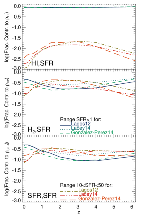
Figure 11: Fractional contribution to the global density of HI (top panel), H₂ (middle panel) and SFR (bottom panel) from galaxies in two bins of SFR, SFR$<0.1\,M_{\odot}\,\rm yr^{-1}$, as labelled in the middle panel, and $10\,M_{\odot}\,{\rm yr}^{-1}<{\rm SFR}<50\,M_{\odot}\,\rm yr^{-1}$, as labelled in the bottom panel, for the Lagos12, Lacey14 and Gonzalez-Perez14 models, as a function of redshift.

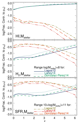
Figure 12: As in Fig. 11, but for galaxies in two bins of stellar mass, $M_{\rm stellar}<10^{8}\,M_{\odot}$, as labelled in the middle panel, and $10^{10}\,M_{\odot}<M_{\rm stellar}<10^{11}\,M_{\odot}$, as labelled in the bottom panel.

One of the aims we have when analysing different GALFORM models is to get a better insight into how much variation we expect in the predicted contributions from galaxies selected according to their stellar mass or SFR to the densities of HI and H₂. This also helps to illustrate how some physical processes, other than the SF law, affect the predictions described in $\S$ 4. From this, it is also possible to identify how robust the trends described in $\S$ 4 are.

Fig. 11 shows the fractional contribution from galaxies in two different bins of SFR to the densities of HI, H₂ and SFR in the Lagos12, Lacey14 and Gonzalez-Perez14 models. The bins were chosen to match those of Fig. 6. We regard the following trends as robust as they are present in all three models: (i) galaxies with low SFRs dominate $\rho_{\rm HI}$, while for $\rho_{\rm H_{2}}$ and $\rho_{\rm SFR}$, they make a modest contribution that decreases from $z=0$ to $z\approx 2.5$, (ii) galaxies with high SFRs have a contribution to $\rho_{\rm HI}$ that increases with increasing redshift, at least up to $z\approx 2.5$, but that never reach more than few percent, for $\rho_{\rm H_{2}}$. Their contribution is of $\approx 8-15$% at $z\sim 0$, increasing to $\approx 25-40$% at $z\approx 1-2.5$, and for $\rho_{\rm SFR}$ their contribution increases with redshift up to $z\approx 1.5$ and stays relatively constant at higher redshifts. Note that the exact peak and normalisation of the contributions of each model sample to the densities of HI, H₂ and SFR depend on the model.

Fig. 12 shows the fractional contribution from galaxies in two different bins of stellar mass to $\rho_{\rm HI}$, $\rho_{\rm H_{2}}$ and $\rho_{\rm SFR}$ in the Lagos12, Lacey14 and Gonzalez-Perez14 models. The bins were chosen to match those of Fig. 6. Here, the following trends are robust: (i) $\rho_{\rm HI}$ has always a large contribution from low mass galaxies that increases with increasing redshift; for H₂, this contribution is negligible at $z\lesssim 2$, but becomes systematically more important at higher redshifts, and for $\rho_{\rm SFR}$ they contribute less than $10$% at $z\lesssim 3.5$, increasing slightly their contribution at higher redshifts; (ii) more massive galaxies ($M_{\rm stellar}>10^{10}\,M_{\odot}$) are never important contributors to $\rho_{\rm HI}$, but host most of the H₂ in the universe at $z\lesssim 3$; in the case of $\rho_{\rm SFR}$, they make more than $30$% of the total SFR at $z\lesssim 3.5$, percentage that slowly decreases at higher redshifts. The exact normalisations of $\rho_{\rm HI,m}$ and $\rho_{\rm H_{2},m}$ slightly vary between the three different models. The largest differences obtained for the contribution to $\rho_{\rm HI}$, $\rho_{\rm H_{2}}$ and $\rho_{\rm SFR}$ from different selections in SFR are seen at $z\gtrsim 4$.

5 Implications for the next generation of galaxy surveys

In this section we discuss the implications of the results presented in $\S$ 4 for the current and next generation of galaxy surveys that aim to detect gas in galaxies. We first focus on the atomic content of galaxies in $\S$ 5.1 and then on the molecular gas in $\S$ 5.2.

5.1 Atomic hydrogen in high-redshift galaxies

Table 1: The fraction of galaxies in the Lagos12 model that have HI velocity-integrated fluxes larger than $3$ times the 1$\sigma$ sensitivity limits, $S_{\rm HI,lim}$ (column $1$), of $4$ different surveys discussed in $\S$ $5.1$, and that have stellar masses $<10^{8}\,M_{\odot}$, SFR$<0.1\,M_{\odot}\,\rm yr^{-1}$ or IR luminosities $<10^{9}\,L_{\odot}$, for different redshifts that cover the redshifts explored by the surveys (columns $2$ to $6$). The numbers in each column are the fraction of galaxies fulfilling the condition of a $>3\sigma$ detection at the given redshift, given the flux limit, [$M_{\rm stellar}<M_{\star,\rm lim}$; SFR$<$SFR_lim; $L_{\rm IR}<L_{\rm IR,lim}$], where $M_{\star,\rm lim}=10^{8}\,M_{\odot}$, SFR${}_{\rm lim}=0.1\,M_{\odot}\,\rm yr^{-1}$ and $L_{\rm IR,lim}=10^{9}\,L_{\odot}$. The sensitivity limits of the ASKAP surveys given in (1) were calculated by Duffy et al. (2012b) for a bandwith of $3.86\,\rm km\,s^{-1}$, and for LADUMA by Sarah Blyth (priv. communication) for a bandwidth of $3.2\,\rm km\,s^{-1}$.

(1)	(2)	(3)	(4)	(5)	(6)
1$\sigma$ sensitivity in ${\rm mJy\,km\,s^{-1}}$	$z=0.08$	$z=0.17$	$z=0.5$	$z=0.8$	$z=1.1$
0.09 (DINGO DEEP)	[0.86; 0.96; 0.98]	[0.83; 0.94; 0.97]	[0.34; 0.58; 0.88]	-	-
0.2 (DINGO)	[0.85; 0.95; 0.98]	[0.75; 0.9; 0.97]	[0.1; 0.27; 0.78]	-	-
1.592 (WALLABY)	[0.64; 0.85; 0.96]	[0.18; 0.54; 0.88]	-	-	-
0.106 (LADUMA BAND-L)	[0.86; 0.96; 0.98]	[0.83; 0.94; 0.97]	[0.28; 0.53; 0.93]	[0.12; 0.25; 0.77]	[0.02; 0.04; 0.6]

There are two ways of studying HI, (i) through its emission at $21$ cm, either by individually detecting galaxies or stacking them to reach a high signal-to-noise ratio and (ii) through the absorption of the light of a background object by the presence of neutral hydrogen in the line-of-sight. We discuss future surveys in the context of HI in emission and absorption.

HI in emission. Large blind surveys of the $21$ cm emission will be carried out by the next generation of radio telescopes, such as the APERITIF project at the Westerbork Synthesis Radio Telescope, the Australian SKA Pathfinder (ASKAP), the South-African SKA pathfinder MeerKAT (MeerKAT), the Jansky Very Large Array (JVLA) and in the longer term future, the Square Kilometer Array (SKA). One of the key surveys planned with ASKAP is DINGO, in which galaxies up to $z\approx 0.43$, with the key science goal of understanding how the HI content of galaxies co-evolves with other major galactic components, such as stars, dust and halo mass. WALLABY will cover much larger areas in the sky, allowing the understanding of the effect of environment on the HI content of galaxies. At higher redshifts, the Looking At the Distant Universe with the MeerKAT Array survey (LADUMA) plans to detect HI emission in individual galaxies up to $z\approx 1$.

Although these future surveys will provide unprecedented knowledge of the neutral gas in galaxies and its cycle, an important fraction of the HI in the universe is expected to be hosted in galaxies with small HI contents ($M_{\rm HI}<10^{6}\,M_{\odot}$) due to the steep low-mass end of the HI mass function. These masses may even be too small to be detected by ASKAP and MeerKAT. To overcome this problem and estimate the HI mass abundances in galaxies that are not individually detected, it is possible to use intensity mapping or stacking of the $21$ cm emission line (see Pritchard & Loeb 2011 for a review). The main difference in the estimates that can be made with intensity mapping is that what it is inferred is $\rho_{\rm HI}\cdot b_{\rm HI}$ (e.g. Chang et al. 2010; Masui et al. 2013), where $b_{\rm HI}$ is the bias in the clustering of HI selected sources with respect to the expected underlying dark matter distribution, while stacking can infer a value for $\rho_{\rm HI}$ from a parent galaxy sample (e.g. Delhaize et al. 2013; Rhee et al. 2013).

Another additional problem that these future surveys may encounter is the identification of UV, optical and/or IR counterparts. We argue that although to measure the total HI density at a given redshift is an important quantity for galaxy formation theory and cosmology, to be able to measure HI in galaxy populations which are selected by other means, either optical emission lines, broadband photometry, etc., is also valuable as additional constraints that can be put on galaxy formation models. However, even if a galaxy is detected in HI emission, its stellar mass and/or SFR may be too small to be measured, making the task of learning about galaxy formation from these HI surveys more challenging.

HI in absorption. Another solution to the problem of faint HI emission is to observe neutral hydrogen in absorption. This has been extensively used to measure the number density of absorbers of different classes, such as DLAs, Lyman limit systems, etc. (see for example Péroux et al. 2003). The first blind absorption survey in HI is going to be carried out by ASKAP (FLASH). This survey will allow measurements of $\rho_{\rm HI}$ as well as constraints on the evolution of faint HI galaxies by combining the FLASH survey with optical galaxy surveys as discussed above, in the redshift range $0.5<z<1$. Recent HI absorption surveys have started to sample statistically the difference between absorbers around late- and early-type galaxies, as well as galaxies in different environments (Tejos et al. 2013; Tumlinson et al. 2013).

We expect that only a combination of the surveys above (direct detection, absorption studies and stacking) will be able to account for most of the HI in galaxies and determine the exact contribution to $\rho_{\rm HI}$ from galaxies with different properties. We summarise in Table 1 the fraction of galaxies that have low stellar masses, SFRs or IR luminosities but that have HI velocity-integrated fluxes that would be detected at a $>3\sigma$ level by the deep HI surveys we described above. These numbers are intended to show the predicted frequency of HI detections that are likely to have no optical counterpart in large optical and near-IR galaxy surveys. A possible solution to this problem is to follow up these HI sources with deep optical and near-IR observations.

5.2 Molecular hydrogen in high-redshift galaxies

Table 2: The fraction of galaxies in the Lagos12 model that have CO emission line velocity-integrated fluxes in the rotational transitions from 1-0 to 6-5 (column $1$) above a $3\sigma$ flux, with $1\sigma=1\,\rm mJy\,km\,s^{-1}$, and that have stellar masses $<10^{9}\,M_{\odot}$, SFR$<10\,M_{\odot}\,\rm yr^{-1}$ or IR luminosities $<10^{10}\,L_{\odot}$, for different redshifts up to $z=2.8$ (columns $2$ to $7$). The numbers in each column are the fraction of galaxies at the given redshift fulfilling the conditions [$M_{\rm stellar}<M_{\star,\rm lim}$; SFR$<$SFR_lim; $L_{\rm IR}<L_{\rm IR,lim}$], where $M_{\star,\rm lim}=10^{9}\,M_{\odot}$, SFR${}_{\rm lim}=10\,M_{\odot}\,\rm yr^{-1}$ and $L_{\rm IR,lim}=10^{10}\,L_{\odot}$.

(1)	(2)	(3)	(4)	(5)	(6)	(7)
CO transition	$z=0.1$	$z=0.5$	$z=1$	$z=1.5$	$z=2$	$z=2.8$
CO(1-0)	[0.76; 0.99; 0.97]	[0.12; 0.95; 0.81]	[0.0003; 0.71; 0.23]	[$10^{-5}$; 0.33; 0.004]	[$10^{-5}$; 0.06; 0]	[0; 0; 0]
CO(2-1)	[0.81; 0.99; 0.98]	[0.5; 0.98; 0.9]	[0.06; 0.86; 0.6]	[0.01; 0.7; 0.29]	[0.003; 0.4; 0.03]	[0.0002; 0.03; $10^{-5}$]
CO(3-2)	[0.83; 0.99; 0.98]	[0.68; 0.98; 0.93]	[0.22; 0.9; 0.71]	[0.06; 0.78; 0.47]	[0.06; 0.58; 0.14]	[0.02; 0.2; 0.0013]
CO(4-3)	[0.82; 0.99; 0.98]	[0.63; 0.98; 0.93]	[0.27; 0.91; 0.73]	[0.09; 0.8; 0.51]	[0.04; 0.62; 0.2]	[0.008; 0.29; 0.004]
CO(5-4)	[0.82; 0.99; 0.98]	[0.57; 0.98; 0.91]	[0.2; 0.9; 0.7]	[0.06; 0.78;0.46]	[0.02; 0.58; 0.15]	[0.006; 0.22; 0.002]
CO(6-5)	[0.8; 0.99; 0.97]	[0.41; 0.97; 0.88]	[0.04; 0.85; 0.58]	[0.009; 0.68;0.26]	[0.003; 0.42; 0.03]	[0.001; 0.04; 0.0006]
CO(7-6)	[0.82; 0.99; 0.97]	[0.3; 0.96; 0.86]	[0.0006; 0.68; 0.22]	[0.0008; 0.33;0.005]	[0.002; 0.07; 0.0003]	[0.006; 0; 0.0003]

To trace molecular gas, lower order molecule transitions are better, as they are most commonly excited predominantly through collisions (in optically thick media), and they are more easily excited than the higher order molecule transitions. The most used molecule to trace H₂ is CO, which is the most abundant molecule after H₂. However, the condition of optically thick media, that defines the excitation means, may break-down in very low metallicity gas, where the CO lines become optically thin (see Carilli & Walter 2013 for a recent review). Lagos12 find that the number of galaxies with gas metallicities $Z_{\rm gas}<0.01\,Z_{\odot}$ is $<0.05$% for galaxies with IR luminosities $>10^{9}\,L_{\odot}$ in the redshift range $0\leq z\leq 6$. This IR luminosity limit corresponds roughly to a SFR$\sim 0.1\,M_{\odot}\,\rm yr^{-1}$. Thus, our model indicates that CO can be used as a good tracer of H₂ for the galaxies that dominate the H₂ content of the universe, which are those with SFR$>1\,M_{\odot}\,\rm yr^{-1}$ or with $M_{\rm stellar}>10^{10}\,M_{\odot}$. Galaxies in which CO is not a good tracer of H₂ (i.e. those with low gas metallicities) represent only a small contribution to the H₂ content of the universe. The downside of CO is the CO-H₂ conversion factor, which is a strong function of metallicity and other physical conditions in the ISM of galaxies (Boselli et al., 2002). The positive side is that the CO-H₂ conversion factor has started to be systematically explored in cosmological simulations of galaxy formation with the aim of informing how much variation with redshift is expected (Narayanan et al. 2012; Lagos et al. 2012; Popping et al. 2013b).

Blind molecular emission surveys are the best way of studying the cold gas content of galaxies in an unbiased way. However, they require significant time integrations to ensure good signal-to-noise. Alternatively, molecular emission line surveys can be guided by well-known UV, optical, IR and/or radio surveys, with well identified positions and spectroscopic or photometric redshifts. Even if only highly star-forming galaxies are used as guide for follow-up molecular emission line surveys, it is possible to place strong constraints on models of galaxy formation, as we show in $\S$ 4, and to provide new insight into the co-evolution of the different baryonic components of galaxies.

The Atacama Large Millimeter Observatory (ALMA) can currently detect CO(1-0) and CO(2-1) up to $z\approx 0.84$. At $z\gtrsim 1.3$, instruments that are primarily designed to detect atomic hydrogen, such as the JVLA are able to detect the emission from the redshifted frequencies of low-J CO transitions.A good example of this is presented in Aravena et al. (2012), who performed a JVLA blind survey in a candidate cluster at $z\sim 1.5$. Aravena et al. obtained two detections and were able to place constraints on the number density of bright CO($1-0$) galaxies. Similarly, blind CO surveys in small areas of the sky are ongoing using the JVLA and the Plateau de Bureau Interferometer (Walter et al., 2013).

For faint sources, the intensity mapping technique described in $\S$ 5.1 can also be applied to molecular emission. The line confusion from galaxies at different redshifts can be overcome by cross-correlating different molecular and/or atomic emission lines. Different emission lines coming from the same galaxies would show a strong correlation, while emission lines coming from galaxies at different redshift would not be correlated. From this, the quantity that is derived is the two-point correlation function or power spectrum weighted by the total emission in the spectral lines being correlated (see Pritchard & Loeb 2011 for a review). The power of using intensity mapping for CO lines have been shown and discussed for instance by Carilli (2011) and Gong et al. (2011). Carilli argues that intensity mapping of CO lines can be performed with telescopes of small field-of-view at redshifts close or at the epoch of reionisation ($z\sim 3-8$).

Unlike in HI, optical counterparts could be easily identified in the case of individual detection of molecular emission, since they are expected to be bright and have large stellar masses. Table 2 shows the fraction of galaxies in model samples selected by their CO velocity-integrated flux and that have stellar masses $<10^{9}\,M_{\odot}$, SFR$<10\,M_{\odot}\,\rm yr^{-1}$ or IR luminosities $<10^{10}\,L_{\odot}$. These fractions are encouraging as they are generally low compared to HI mass selected samples, particularly at high redshifts; this means that we expect effectively all of the molecular emission lines detected to have detectable optical/IR counterparts. From this, one can conclude that the most efficient strategy to uncover the H₂ in the universe is the follow-up of already existing optical/IR/radio catalogues with submillimeter and/or radio telescopes with the aim of detecting molecular emission lines.

6 Conclusions

We have presented predictions for the contribution to the densities of atomic and molecular hydrogen from galaxies with different stellar masses, SFRs and IR luminosities in the context of galaxy formation in a $\Lambda$CDM framework. We use three flavours of the GALFORM semi-analytic model of galaxy formation, the Lagos12, Gonzalez-Perez14 and Lacey14 models. For quiescent star formation, the three models use the pressure-based SF law of Blitz & Rosolowsky (2006), in which the ratio between the gas surface density of H₂ and HI is derived from the radial profile of the hydrostatic pressure of the disk, and calculates the SFR from the surface density of H₂. The advantage of this SF law is that the atomic and molecular gas phases of the ISM of galaxies are explicitly distinguished. Other physical processes in the three models are different, such as the adopted IMF and the strength of both the SNe and the AGN feedback, as well as the cosmological parameters adopted.

We identify the following trends in the three models and regard them as robust:

(i) The HI density shows almost no evolution at $z\lesssim 2$, and slowly decreases with increasing redshift for $z\gtrsim 2$.

(ii) The H₂ and the SFR densities increase strongly from $z=0$ up to $z\approx 2-3$, followed by a slow decline at higher redshifts. The models predict an increase in SFR larger than for H₂ due to the contribution from starbursts, which is larger for the SFR (close to $50$% in the three models at $z\approx 3$) than for H₂ (less than $10$% at $z\approx 3$). The latter is due to starbursts being on average more efficient at converting gas into stars, and therefore contributing more to the SFR density than the gas density of the universe.

(iii) The three models predict densities of SFR, HI and H₂ in broad agreement with the observations at $z\lesssim 3$. A higher redshifts important deviations are observed between the predicted $\rho_{\rm HI}$ and the observationally inferred values in the three models. We argue that this is not unexpected as the HI in our simulations correspond exclusively to HI in galaxies and no contribution from the HI in the IGM is included. The latter is expected to become important at $z\gtrsim 3$ (van de Voort et al., 2012).

(iv) The density of HI is always dominated by galaxies with low SFR (SFR$<1\,M_{\odot}\,\rm yr^{-1}$), and low stellar masses ($M_{\rm stellar}<10^{9}\,M_{\odot}$), while the H₂ density is dominated by galaxies with relatively large SFRs (SFR$>1\,M_{\odot}\,\rm yr^{-1}$) and large stellar masses ($M_{\rm stellar}>10^{10}\,M_{\odot}$). The latter is also true for the global SFR density.

(v) The predicted evolution of the global SFR density observed in the universe can be largely explained as driven by the steep decline of the molecular mass towards $z=0$. The combination of the evolution of the total neutral gas, atomic and molecular, and the increasing galaxy sizes with decreasing redshift explain the evolution of the H₂ density. The global SFR density evolution can therefore be linked to the evolution of the neutral gas surface density of the galaxies dominating the SFR in the Universe at a given time. The evolution of the neutral gas content of galaxies is set by the balance between inflows and outflows of gas in galaxies, and therefore also plays a key role in the evolution of the molecular gas, that ultimately set the SFR. Thus, one must understand that the H₂ content and SFR of galaxies in the star-forming sequence of the SFR-stellar mass plane are set by the self-regulation of inflow and outflows and that small deviations to this self-regulation produce the time evolution of this sequence.

(vi) We find that a group of observations can be connected and understood in the models, including the H$\alpha$ and UV luminosity functions, distribution function of the global SFR density on stellar mass, the global SFR density from highly star-forming galaxies, the inferred HI density from massive galaxies in the local Universe, and the inferred H₂ density of highly star-forming galaxies at high-redshifts. This broad set of comparisons between observations and model predictions that test at the same time the stellar mass and SFR and the neutral gas content of galaxies is unprecedented in semi-analytic models of galaxy formation.

We discuss our findings in the context of future surveys and suggest that optical identification of faint HI counterparts is going to be difficult due to the low stellar masses and SFRs we expect for them. These faint HI galaxies are, however, key to our understanding of galaxy formation as we expect them to dominate the HI content of the universe. We suggest that stacking techniques are promising to measure the contribution to HI from galaxies selected by their stellar mass or SF activity. Such measurements have the potential to place strong constraints on galaxy formation models. Regarding H₂, the easiest way to make progress is to use current surveys with well identified optical, IR and/or radio positions and well known spectroscopic or photometric redshifts and follow them up with current facilities, with the downside that the selection function becomes more complex to model. The fact that most of the H₂ is predicted by our model to be hosted by relatively massive, star-forming galaxies, which are already detectable by optical and IR surveys, it is implied that follow-up surveys will be able to uncover the H₂ density of the universe without the need of blind surveys. From such observations, it is implied that both direct detection and stacking would provide valuable information on the cold gas content of galaxies and place strong constraints on galaxy formation models.

Appendix A Scaling stellar masses and star formation rates to our adopted IMF

Due to our chose of the Kennicutt (1983) IMF, we have to scale the observational inferences of stellar masses and SFRs made with other choices of IMF. The other choices of IMFs in the compilation of data presented in Fig. 3 and Fig. 4 are the Chabrier (2003) IMF, the Salpeter (1955) IMF and the Baldry & Glazebrook (2003) IMF.

For stellar masses, we follow the conversions in Table 3 that have been taken from Bell et al. (2003) and Gilbank et al. (2010).

Table 3: Scaling of the stellar mass from different IMF choices to a Kennicutt (1983) IMF. The conversion given for each IMF follows $M^{\rm Kenn}_{\rm stellar}={\rm corr}\,\cdot M^{\rm IMF}_{\rm stellar}$, where $M^{\rm Kenn}_{\rm stellar}$ is the stellar mass inferred for a Kennicutt (1983) IMF and $M^{\rm IMF}_{\rm stellar}$ the stellar mass inferred in observations that adopted a different IMF. These are taken from the work of Bell et al. (2003) and Gilbank et al. (2010).

IMF	corr
Salpeter (1955)	0.5
Chabrier (2003)	0.89
Baldry & Glazebrook (2003)	2.25

The case of SFRs is more complex than the stellar mass, since the conversion depends on the SFR tracer used. We here follow the scalings calculated by Gonzalez-Perez et al. (2013, in prep.). Gonzalez-Perez et al. use the PEGASE (Fioc & Rocca-Volmerange, 1999), and assume a constant solar etallicity and SFR to calculate the H$\alpha$, H$\beta$, [OII], FUV and radio luminosities for each choice of IMF. Note, however, that the conversions are subject to systematics related to the assumptions of SF history and metallicity (e.g. Wilkins et al. 2012). We summarise in Table 4 the scalings applied to each observationally inferred SFR depending on the adopted IMF and used tracer to convert to a Kennicutt (1983) IMF. Here, FUV corresponds to a filter centered at $1500$Å and width $400$Å and NUV to a filter centered at $2000$Å and width $400$Å.

Table 4: Scaling to convert the observationally inferred SFR that adopted an IMF different than the Kennicutt (1983) IMF. The conversion given for each IMF follows ${\rm SFR}^{\rm Kenn}={\rm corr}\,\cdot{\rm SFR}^{\rm IMF}$, where ${\rm SFR}^{\rm Kenn}$ would be the SFR inferred for a Kennicutt (1983) IMF and ${\rm SFR}^{\rm IMF}$ the SFR inferred in observations that adopted a different IMF. Each column shows a different SFR tracer.

IMF	optical E.L.	1500Å	2000Å
Salpeter (1955)	0.93	0.79	0.77
Chabrier (2003)	1.57	1.26	1.22
Baldry & Glazebrook (2003)	2.26	1.56	1.63
Top-heavy IMF ($x=1$)	3.132	1.892	1.772
IMF	2500Å	2800Å	3550Å
Salpeter (1955)	0.76	0.747	0.717
Chabrier (2003)	1.203	1.172	1.11
Baldry & Glazebrook (2003)	1.445	1.385	1.266
Top-heavy IMF ($x=1$)	1.771	1.616	1.434
IMF	FIR	radio
Salpeter (1955)	0.807	0.77
Chabrier (2003)	1.296	1.22
Baldry & Glazebrook (2003)	1.636	1.46
Top-heavy IMF ($x=1$)	2.022	1.678

Appendix B The local universe HI and H₂ mass functions

In Fig. 13 we show the predicted HI and H₂ mass functions at $z=0$ for the Lagos12, Lacey14 and Gonzalez-Perez14 models. We compare with observations of the HI mass function from Zwaan et al. (2005) and Martin et al. (2010), and of the inferred H₂ mass function from Keres et al. (2003). The latter observations correspond to CO($1-0$) molecular emission line in galaxies that were previously selected from their emission in the $B$-band or $60\mu$m. We then use a Milky-Way type conversion between the CO($1-0$) emission and the H₂ mass, and infer a H₂ mass function. We showed in Lagos et al. (2012) that doing the opposite exercise of converting predicted H₂ masses to CO($1-0$) emission using radiative transfer, photon dominated region codes to calculate the CO-H₂ conversion factor, leads to similar CO($1-0$) luminosity function than the one obtained by assuming a constant conversion factor. This is due to the fact that most model galaxies at $z=0$, which have CO($1-0$) luminosities above the observational limit of Keres et al. (2003), have gas metallicities and SFR densities that are not too different from normal spiral galaxies. The three models give predictions that are in good agreement with the observations.

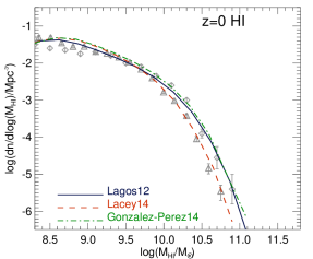
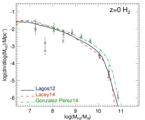
Figure 13: Top panel: The HI mass function at $z=0$ for the Lagos12, Lacey14 and Gonzalez-Perez14 models, as labelled. Symbols show observational results at $z=0$ from Zwaan et al. (2005) using HIPASS (diamonds) and Martin et al. (2010) using ALFALFA (squares). Bottom panel: Same as the top panel but for H₂. Here we show observational inferences from Keres et al. (2003) using direct detection of the $\rm CO(1-0)$ emission line in $B$-band (triangles) and $60\,\mu$m (filled circles) selected samples of galaxies. The observational mass function is then calculated assuming the Milky Way $\rm H_{2}$-to-CO conversion factor, $N_{\rm H_{2}}/\rm cm^{-2}=2\times 10^{-20}\,I_{\rm CO}/\rm K\,km\,s^{-1}$. Here $N_{\rm H_{2}}$ is the column density of H₂ and $I_{\rm CO}$ is the integrated CO$(1-0)$ line intensity per unit surface area.

Appendix C The dark matter halos of the Lagos12, Lacey14 and Gonzalez-Perez14 models

C.1 The Lagos12, Lacey14 and Gonzalez-Perez14 models in the Millennium database

The predictions of the three GALFORM models used in this paper will be publicly available from the Millennium database. However, the reader should keep in mind that the runs performed in this paper are not ‘standard’ in the sense that we use Monte-Carlo realisations of a wider dynamical range of halo masses compared to the $N$-body simulations Millennium (Springel et al., 2005), used by the Lagos12 model, and MS-W7 (same as the Millennium simulation but with WMAP7 cosmology), used by Gonzalez-Perez14 and Lacey14. This means that the runs shown in this paper follow the formation of galaxies in dark matter halos that extend to much lower masses than the two $N$-body simulations above. The minimum halo mass of the Millennium and MS-W7 simulations is fixed on $1.72\times 10^{10}\,h^{-1}\,M_{\odot}$. This has the limitation that the results presented here for the HI density cannot be fully reproduced with the galaxies in the Millennium database. This is due to the faint nature of the galaxies that dominate $\rho_{\rm HI}$, which are hosted by dark matter halos that are not resolved in the Millennium and MS-W7 $N$-body simulations. All the results related to H₂ and SFR density (including the H$\alpha$ and UV luminosity functions) can be reproduced using the galaxies in the Millennium database at $z<4$. This is because the galaxies that dominate these statistical measurements are relatively massive, and hosted by halos that are well resolved in the $N$-body simulations. At $z>4$, the SFR density is not fully resolved in the resolution of the Millennium and MS-W7 $N$-body simulations.

We have also performed runs using the dark matter halo merger trees of the Millennium-II simulation, which has a minimum halo mass fixed at $1.38\times 10^{8}\,h^{-1}\,M_{\odot}$ (Boylan-Kolchin et al., 2009). We find that the dynamical range of the Millennium-II is sufficient to resolve the HI in galaxies at $z\lesssim 2.5$. However, at higher redshifts, the Millennium-II misses the lowest halo masses that still contribute to the HI in the universe ($10^{7}-10^{8}\,h^{-1}\,M_{\odot}$), that are covered by our Monte-Carlo merger trees thanks to the redshift scaling applied to the minimum halo mass.

C.2 Resolution tests

Table 5: Simulations used to test the convergence of the predictions of the models. Column (1) gives the name of each simulation, (2) the minimum halo mass adopted, $M_{\rm halo,min}$, and (3) the scaling of the minimum halo mass with redshift. The standard simulation used throughout the manuscript is r3.

Simulation	$M_{\rm halo,min}/M_{\odot}\,h^{-1}$	Scaling
r1	$10^{10}$	$(1+z)^{-3}$
r2	$5\times 10^{9}$	$(1+z)^{-3}$
r3	$5\times 10^{8}$	$(1+z)^{-3}$
r4	$2.5\times 10^{8}$	$(1+z)^{-3}$
r5	$10^{10}$	no scaling
r6	$5\times 10^{9}$	no scaling

A questions that comes immediately from the lack of resolution in the Millennium and MS-W7 $N$-body simulations is whether the results presented here for the HI density are converged or not. To answer this question, we performed a simple exercise: we run the same model under $6$ different resolutions, with and without the scaling with redshift of the minimum halo mass. Table 5 summarises the different runs. The scaling with redshift is also changed to study the effect of this scaling on the HI density to reproduce the conditions of the $N$-body runs (i.e. fixed minimum halo mass) and also to show the importance of adding the redshift scaling in the Monte-Carlo merger trees. Fig. 14 shows a visualization of the different resolutions of all the runs. We also show in Fig. 14 the resolution of the Millennium I and Millennium II $N$-body simulations.

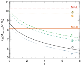
Figure 14: The minimum halo mass in the different resolution runs as a function of redshift. The lines correspond to the r1 (dot-dashed line), r2 (dashed line), r3 (solid line), r4 (dotted line), r5 (horizontal triple dot-dashed line) and r6 (horizontal dotted line) runs. As a reference, we also show the resolution of the Millennium I (horizontal long dashed line) and Millennium II (horizontal solid line) simulations.

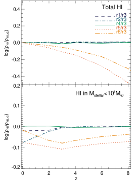
Figure 15: The ratio between the HI density in a given resolution and the r3 run, as a function of redshift. The top panel shows the global HI density ratio and the bottom panel shows the HI density in galaxies with $M_{\rm stellar}<10^{8}\,M_{\odot}$ in the Lagos12 model. Each line shows a different resolution test as labelled with respect to our standard run, the r3 resolution.

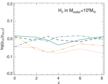
Figure 16: Same as the bottom panel of Fig. 15 but for H₂.

We show in Fig. 15 the global HI density and the contribution to it from galaxies with $M_{\rm stellar}<10^{8}\,M_{\odot}$ for the Lagos12 model in the five Monte-Carlo tree resolutions, all normalised to our standard choice, the ‘r3’ Monte-Carlo merger trees. By comparing the r3 with the r4 resolution, we can conclude that our standard resolution (r3) is converged to a factor better than $2$%. When comparing the resolutions r1 and r2 with our standard r3 resolution, we conclude that although the global HI density is converged to a factor better than $10$%, the contribution from low mass galaxies is not. This is shown in the bottom panel of Fig. 15, where r1 and r2 predict lower contributions from the low mass galaxies to $\rho_{\rm HI}$ by $\approx 60$% and $\approx 10$%, respectively. The importance of the redshift scaling introduced in the minimum halo mass in our standard run is crucial to make our predictions converge. This can be concluded from the large offset between the r3 and the runs r5 and r6, which increases with increasing redshift. Lagos et al. (2011a) argue that this is the reason why previous models predict a monotonically increasing H${}_{2}/$HI global density ratio with increasing redshift (e.g. Obreschkow et al. 2009; Popping et al. 2013a), and miss the turnover in this ratio, which takes place at $z\approx 5$ (i.e. in the regime where the fixed resolution run largely underestimates the global HI density). Also note that the runs r5 ad r6 predict a $\rho_{\rm HI}$ that converges to the high-resolution $\rho_{\rm HI}$ at $z\lesssim 1$. The contribution from low mass galaxies ($M_{\rm stellar}<10^{8}\,M_{\odot}$) to the density of H₂, shown in Fig. 16 is converged to better than $10$% at the resolution of r2, meaning that the contribution from small galaxies is resolved in or standard simulation. The fact that the convergence is achieved at lower resolutions compared to the case of HI is due to the flatter low-mass end of the H₂ mass function compared to the steepness of the low-mass end of the HI mass function.

References

- Altay et al. (2011) Altay G., Theuns T., Schaye J., Crighton N. H. M., Dalla Vecchia C., 2011, ApJ, 737, L37
- Aravena et al. (2012) Aravena M., Carilli C. L., Salvato M., Tanaka M., Lentati L., Schinnerer E., Walter F., Riechers D. et al, 2012, MNRAS, 426, 258