Direct measurements of dust attenuation in $z\sim 1.5$ star-forming galaxies from 3D-HST:
Implications for dust geometry and star formation rates

Abstract

The nature of dust in distant galaxies is not well understood, and until recently few direct dust measurements have been possible. We investigate dust in distant star-forming galaxies using near-infrared grism spectra of the 3D-HST survey combined with archival multi-wavelength photometry. These data allow us to make a direct comparison between dust around star-forming regions ($A_{\mathrm{V\!,\,\textsc{Hii}}}$) and the integrated dust content ($A_{\mathrm{V\!,\,star}}$). We select a sample of 163 galaxies between $1.36\leq{}z\leq 1.5$ with $\mathrm{H\alpha}$ signal-to-noise ratio $\geq 5$ and measure Balmer decrements from stacked spectra to calculate $A_{\mathrm{V\!,\,\textsc{Hii}}}$. First, we stack spectra in bins of $A_{\mathrm{V\!,\,star}}$, and find that $A_{\mathrm{V\!,\,\textsc{Hii}}}=1.86\,A_{\mathrm{V\!,\,star}}$, with a significance of $\sigma=1.7$. Our result is consistent with the two-component dust model, in which galaxies contain both diffuse and stellar birth cloud dust. Next, we stack spectra in bins of specific star formation rate ($\log\,\mathrm{SSFR}$), star formation rate ($\log\,\mathrm{SFR}$), and stellar mass ($\log{}M_{*}$). We find that on average $A_{\mathrm{V\!,\,\textsc{Hii}}}$ increases with SFR and mass, but decreases with increasing SSFR. Interestingly, the data hint that the amount of extra attenuation decreases with increasing SSFR. This trend is expected from the two-component model, as the extra attenuation will increase once older stars outside the star-forming regions become more dominant in the galaxy spectrum. Finally, using Balmer decrements we derive dust-corrected $\mathrm{H\alpha}$ SFRs, and find that stellar population modeling produces incorrect SFRs if rapidly declining star formation histories are included in the explored parameter space.

1. Introduction

While dust makes up only a very small fraction of the baryonic mass in galaxies (Draine et al., 2007), it leaves a large signature on their spectral energy distributions (SEDs). Dust extinguishes light in a wavelength-dependent way, and therefore distorts the intrinsic SED of galaxies. This distortion, or net dust attenuation, may depend on the properties of the dust, the dust-to-star geometry, or both quantities. Therefore, recovering the intrinsic stellar SEDs from observations requires a thorough understanding of both factors.

Dust properties and geometry are studied using observations of both dust emission and attenuation. Studies of dust emission at mid- and far-infrared wavelengths have placed constraints on the composition, distribution, and mass of dust in nearby galaxies (e.g., Draine et al., 2007; Galliano et al., 2008; Dale et al., 2012). Measurements of dust attenuation are also needed to completely characterize the nature of dust, including the dust-to-star geometry.

One method of constraining the dust-to-star geometry is by comparing the integrated dust attenuation with the attenuation towards star-forming (SF) regions. Dust attenuation affecting the stellar continuum, $A_{\mathrm{star}}$, has been measured using a number of methods. These include (i) line of sight measurements (e.g., the MW, SMC, LMC), (ii) matching attenuated galaxies with unattenuated galaxies with similar intrinsic stellar populations (i.e. Calzetti et al., 2000; Wild et al., 2011), (iii) fitting the SED with stellar population synthesis models, including a prescription for dust, and (iv) the $L_{\mathrm{IR}}/L_{\mathrm{UV}}$ ratio (also known as IRX), which probes dust attenuation using energy conservation. The latter ratio is directly related to the UV continuum slope $\beta$ (Meurer et al., 1999), which may be used to infer the dust content for galaxies for which no IR data is available. (See Conroy 2013 for more discussion on this topic).

Dust attenuation towards SF regions, $A_{\mathrm{\textsc{Hii}}}$, has also been extensively studied in low-redshift galaxies. $A_{\mathrm{\textsc{Hii}}}$ is most directly probed with recombination line flux ratios, often using the Balmer decrement H$\alpha$/$\mathrm{H\beta}$. The intrinsic line ratio can be calculated given reasonable environmental parameters. As dust attenuation is wavelength dependent, the measured line ratio compared with the intrinsic ratio combined with an assumed dust law yields a measure of the amount of dust attenuation towards SF regions. This method was used by a number of studies to measure attenuation towards SF regions in nearby galaxies (e.g., Calzetti et al., 2000; Brinchmann et al., 2004; Garn & Best, 2010).

By comparing $A_{\mathrm{V\!,\,\textsc{Hii}}}$ and $A_{\mathrm{V\!,\,star}}$, Calzetti et al. (2000) find that there is extra dust attenuation towards star-forming regions relative to the integrated dust content for local starburst galaxies. Wild et al. (2011) expand on this work by finding that the amount of extra attenuation increases with the axial ratio and decreases with SSFR. This implies that the dust content of galaxies might have two components (e.g., Calzetti et al., 1994; Charlot & Fall, 2000; Granato et al., 2000): a component associated with the short-lived birth clouds in SF regions and a diffuse component distributed throughout the ISM. In this model, the diffuse dust attenuates light from all stars, while the birth cloud dust component only attenuates light originating from the SF region.

At higher redshifts, the nature of dust attenuation is much more poorly understood. Much of the work on dust attenuation in high-$z$ galaxies has focused on the UV slope (e.g., Reddy et al., 2006, 2010; Wilkins et al., 2011; Bouwens et al., 2012; Finkelstein et al., 2012; Reddy et al., 2012; Hathi et al., 2013, also see Shapley 2011 for a comprehensive review), as it is relatively easy to observe. However, deviations from the Meurer et al. (1999) IRX-$\beta$ relation have been found for various galaxy samples (e.g., Kong et al., 2004; Johnson et al., 2007; Conroy et al., 2010; Gonzalez-Perez et al., 2013). Additional methods of measuring attenuation in high-$z$ galaxies include SED modeling of photometric or spectroscopic observations (e.g., Buat et al., 2012; Kriek & Conroy, 2013) andcomparison of star formation rate (SFR) indicators (e.g., Wuyts et al., 2013).

Direct measurements of dust attenuation toward Hii regions using Balmer decrements are very challenging for $z>0.5$ as both $\mathrm{H\alpha}$ and $\mathrm{H\beta}$ are shifted to the less-accessible near-infrared window. Careful survey design and instrument improvements have made measurements of the Balmer decrement possible for larger samples of intermediate redshift galaxies, e.g., between $0.4\lesssim z\lesssim 1$ (Savaglio et al., 2005), $z\sim 0.5$ (Ly et al., 2012), and $z\sim 0.8$ (Villar et al., 2008; Momcheva et al., 2013). However, until recently Balmer decrements have been measured for only a small number of more distant galaxies (e.g., Teplitz et al., 2000; van Dokkum et al., 2005; Hainline et al., 2009; Yoshikawa et al., 2010).

Interestingly, current studies of dust properties in distant star-forming galaxies yield contrasting results. Erb et al. (2006b) and Reddy et al. (2010) find that extra attenuation towards Hii regions leads to an overestimate of the $\mathrm{H\alpha}$ SFR relative to the UV slope SFR. However, Förster Schreiber et al. (2009) compare measured and predicted $L_{\mathrm{H\alpha}}$ and $\mathrm{H\alpha}$ equivalent widths and find the best agreement when $A_{\mathrm{V\!,\,\textsc{Hii}}}$ includes extra attenuation relative to $A_{\mathrm{V\!,\,star}}$. A comparison of overlapping objects with Erb et al. (2006b) shows that the previous aperture corrections might be overestimated, which could have masked some extra attenuation. Yoshikawa et al. (2010) compare $A_{\mathrm{V\!,\,star}}$ from SED fitting and $A_{\mathrm{V\!,\,\textsc{Hii}}}$ from Balmer decrements for a small sample and find that the high-$z$ objects are consistent with the local universe Calzetti et al. (2000) prescription for extra dust attenuation. Additionally, Wuyts et al. (2011b; 2013), Mancini et al. (2011) and Kashino et al. (2013) find the best agreement between $\mathrm{H\alpha}$ SFRs and UV+IR/SED SFRs when extra attenuation is adopted, either the same as the Calzetti et al. (2000) relation (Wuyts et al., 2011b; Mancini et al., 2011) or a slightly lower ratio (Wuyts et al., 2013; Kashino et al., 2013). Kashino et al. (2013) also measure the Balmer decrement and find the amount of extra attenuation is lower than the Calzetti et al. (2000) relation.

These contrasting results may not be surprising, given the different and indirect methods and/or small and biased samples of most studies. Direct measurements of a statistical sample of distant galaxies are required to clarify these dust properties. This is now possible, as new NIR instruments with multiple object spectroscopy capabilities are able to measure the Balmer decrement for larger and more complete samples of high-redshift objects. In particular, the Hubble Space Telescope’s WFC3/G141 grism filter provides slit-less spectra, allowing for a non-targeted survey of a large number of high-redshift galaxies. The HST grisms also avoid atmospheric near-IR absorption.

A number of surveys, including the 3D-HST survey (van Dokkum et al., 2011; Brammer et al., 2012), CANDELS (Koekemoer et al., 2011), and the WISP survey (Atek et al., 2010), have taken advantage of the HST grism capabilities to survey high redshift galaxies. Domínguez et al. (2013) were the first to use WFC3 grism data to make measurements of the Balmer decrement on a large, non-targeted sample. However, as their sample was not drawn from regions of the sky with existing deep photometric coverage, they were unable to examine trends of dust versus integrated galaxy properties.

We present a statistical study of dust attenuation measured using the Balmer decrement for a large, non-targeted sample of galaxies at $z\sim 1.5$. Both rest-frame optical spectra and deep photometry are available, allowing us to compare attenuation towards Hii regions with the total integrated dust attenuation and other galaxy properties, including stellar mass and SFR.

Throughout this paper we adopt a $\Lambda$CDM universe with $\Omega_{m}=0.3$, $\Omega_{\Lambda}=0.7$, and $H_{0}=70\ \mathrm{km\,s^{-1}\,Mpc^{-1}}$.

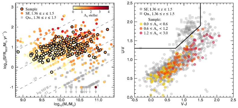
Figure 1.— Sample characteristics relative to all 3D-HST galaxies in the same redshift range. The left panel shows $\log M_{*}$ vs. log SFR (from SED fitting) for all 3D-HST galaxies at $1.36\leq z\leq 1.5$. The black circles indicate the sample selected for direct Balmer decrement measurements, consisting of galaxies with a strong $\mathrm{H\alpha}$ detection (i.e. S/N $\geq$ 5). Colors indicate the stellar $A_{\mathrm{V}}$ of the best-fit SED models found using the grism spectra and the photometry, as described in Section 2.1. The grey dashed lines show constant values of log SSFR. The right panel presents the rest-frame U-V and V-J colors for all 3D-HST galaxies between $1.36\leq z\leq 1.5$ (in grey) and our sample (color-coded by stellar $A_{\mathrm{V}}$ bin). We discard any galaxies lying within the quiescent box (using the definition from Whitaker et al. 2012a) from our sample, as the emission lines for these galaxies likely originate from AGNs. In both panels, objects within the quiescent box of the UVJ diagram are shown as grey squares, while star-forming objects are shown as circles.

2. Data

2.1. Observations and catalog

Our sample is drawn from the 3D-HST survey (Brammer et al., 2012), a Hubble Space Telescope (HST) Treasury program adding ACS and WFC3 slit-less grism observations to the well-covered CANDELS (Koekemoer et al., 2011) fields: AEGIS, COSMOS, GOODS-S, and UDS. The 3D-HST data also include observations of the GOODS-N field from program GO-11600 (PI: B. Weiner).

In this work we use the 3D-HST WFC3/G141 grism spectra, which cover $1.1\mathrm{\mu m}<\lambda<1.65\mathrm{\mu m}$. The raw grism dispersion is $46.5\,\mathrm{\AA\,pixel^{-1}}$, but interlacing during data reduction improves the dispersion to $\sim\!23\,\mathrm{\AA\,pixel^{-1}}$ (corresponding to about 10 restframe $\mathrm{\AA\,pixel^{-1}}$ for $z\sim 1.5$). The G141 grism has a maximum resolution of $R\sim 130$, corresponding to $\sim 110\,\mathrm{\AA}$ in the middle of our wavelength range.

The 3D-HST survey makes use of existing deep photometric coverage in each of the survey fields, combining the grism spectra with multi-wavelength photometric data. The 3D-HST photometric catalogs are discussed in detail in Skelton et al. (2014). This work uses version 2.1 of the photometric and grism catalogs.

A modified version of the Eazy code (Brammer et al., 2008) is used on the combined grism spectra + photometry to measure the redshifts, emission line fluxes, and rest-frame U, V, J fluxes of the individual 3D-HST galaxies. Stellar masses, integrated dust attenuation, SFRs, and specific star formation rates (SSFRs) are determined by fitting stellar population synthesis models to the photometric data using the FAST code (Kriek et al., 2009). We use a separate set of parameters than those used by Brammer et al. (2012), for reasons discussed in Section 4.4. We use the Bruzual & Charlot (2003) stellar population synthesis models, assuming a Chabrier (2003) stellar initial mass function, solar metallicity, an exponentially declining star formation history with a minimum e-folding time of $\log_{10}(\tau_{\mathrm{min}}/\mathrm{yr})=8.5$, a minimum age of 40 Myr, and an integrated dust attenuation $A_{\mathrm{V}}$ between 0 and 4 assuming the dust attenuation law by Calzetti et al. (2000).

Brammer et al. (2012) provide complete details on the 3D-HST survey data reduction and parameter measurement procedure.

2.2. Sample selection

We select galaxies in the redshift range $1.36\leq z\leq 1.5$, for which $\mathrm{H\alpha}$ and $\mathrm{H\beta}$ are generously covered by the G141 grism. In addition we impose a signal-to-noise ratio (SNR) cut for $\mathrm{H\alpha}$ of SNR $\geq 5$, to measure a decent line signal. We make no $\mathrm{H\beta}$ SNR cut, to avoid biasing our sample against the dustiest galaxies.

We have a number of additional selection criteria, to ensure high quality of the spectra. First, to avoid cases of line misidentification, the photometric-only and grism+photometry redshifts (hereafter referred to as the grism redshifts) must have good agreement, i.e. $|z_{\mathrm{phot}}-z_{\mathrm{grism}}|\leq 0.2$. Second, the contamination from other sources (which is an issue because of the slit-less nature of the grism spectra) may not exceed 15%. Third, there must be grism coverage of at least 95% and must include the $\mathrm{H\alpha}$ and $\mathrm{H\beta}$ lines. Fourth, no more than 50% of the spectrum may be flagged as problematic (due to bad pixels or cosmic rays) during reduction.

To study dust attenuation towards star forming regions, we do not want AGN to contaminate our emission lines. To reject AGN, we exclude any objects that have a detected X-ray luminosity $L_{X}>10^{42}\,\mathrm{erg\;s^{-1}}$ (Mendez et al., 2013; Rosario et al., 2013; Bauer et al., 2002) by matching against the Chandra Deep Field North and South surveys (Alexander et al., 2003; Xue et al., 2011) and the XMM-Newton serendipitous survey (Watson et al., 2009). Furthermore we reject all objects that fall within the Donley et al. (2012) IRAC AGN region, or that fall within the quiescent box in the UVJ diagram defined in Whitaker et al. (2012a) (as the line emission likely originates from an AGN).

Finally, we visually inspect the grism spectra and photometry of the preliminary sample to reject problematic objects (i.e. objects with incorrect line identification or poor quality broadband photometry). Our final sample includes 163 galaxies. Figure 1 shows how our sample compares to the full galaxy distribution at a similar redshift. The selected galaxies all have relatively high SFRs, and lie along the “star-forming main sequence” (e.g., Noeske et al., 2007b; Daddi et al., 2007; Wuyts et al., 2011a; Whitaker et al., 2012b; Nelson et al., 2013).

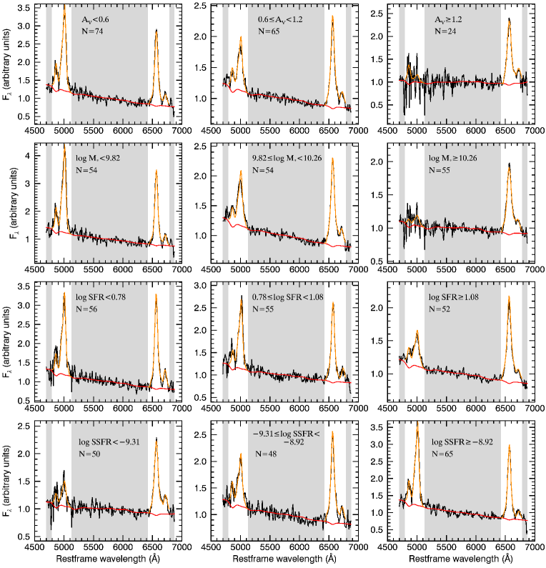
Figure 2.— Stacked spectra for bins in stellar $A_{\mathrm{V}}\!$ (top), $\log M_{*}$ (second row), log SFR (third row) and log SSFR (bottom). In each panel, the stacked spectrum is plotted in black, with the continuum fit shown in red. The best-fit line measurements (from shortest to longest wavelength: $\mathrm{H\beta}$, [OIII]$\lambda\lambda 4959,5007\mathrm{\AA}$, blended H$\alpha$+[NII]$\lambda\lambda 6548,6584\mathrm{\AA}$, and [SII]$\lambda\lambda 6717,6731\mathrm{\AA}$) are shown in orange. The additional continuum correction is done by fitting the portions of the spectra within the shaded grey regions.

2.3. Stacking

The spectra of individual galaxies in this sample are too noisy to yield a clear measurement of the Balmer decrement, the ratio of the flux of $\mathrm{H\alpha}$ to $\mathrm{H\beta}$ ($F_{\mathrm{H\alpha}}/F_{\mathrm{H\beta}}$). Thus, we bin galaxies by parameter (SED $A_{\mathrm{V}}$, SSFR, SFR, stellar mass) and stack the spectra before measuring line fluxes.

Prior to stacking, we scale the spectra to match the photometry, as the spectra and photometry have a slightly different slope for most galaxies. A linear correction for this effect is calculated during the reduction stage, and we apply this linear correction to the individual grism spectra. Individual spectra are also corrected for contamination from other sources during the reduction process.

We adopt a uniform methodology for stacking spectra within a bin. First, we only use the portion of the grism spectra that falls between $1.13\mathrm{\mu m}$ and $1.65\mathrm{\mu m}$ (observed wavelength) to avoid noise at the edge of the grism coverage. Then the individual spectra are continuum normalized by scaling the biweighted mean value of the flux between $5500-6000\mathrm{\AA{}}$ (rest-frame) to unity. The individual spectra are then interpolated onto a common rest-frame wavelength grid.

The normalized, interpolated spectra are stacked at each wavelength. For each bin, simulated spectra ($N=500$) are generated by perturbing the individual spectra, assuming that the flux errors are normally distributed, and then stacking the perturbed spectra using the same procedure as above. The simulated spectra are used in determining the errors of the emission lines (see Section 2.4).

The best-fit stellar population models are sampled over the same wavelength regime as the original spectra and used as the continua. The best fits are stacked in the same way: they are continuum normalized and interpolated onto a common rest-frame wavelength grid, then averaged together. We then convolve the stacked continua models with the stacked line profiles (discussed in Section 2.4) to match the resolution of the grism spectra.

To estimate the error in the continua, we perturb the photometry of an object and determine the FAST best-fit model for each perturbation. This procedure is repeated a number of times for each object. Within each bin, we randomly select a best-fit model to the perturbed photometry for each object and stack to construct a simulated continuum. This procedure is repeated 500 times, in order to create a continuum model for each simulated spectrum, as discussed above. The average photometry and stacked best-fit models with errors are shown in the Appendix.

Finally, we apply a second-order polynomial correction between the stacked grism spectra and the stacked best-fit stellar population continua, to further correct for possible mismatches. This small change corrects for otherwise uncharacterized differences across the grism spectra. The corrected, stacked spectra and continua for the different bins are shown in Figure 2.

The adopted continuum normalization scheme leads objects with higher scaled $\mathrm{H\alpha}$+[NII] (see Section 2.4) fluxes to have more weight in our line stack. To correctly compare the parameters from SED fitting ($A_{\mathrm{V\!,\,star}}$, stellar mass, SFR, SSFR) with values calculated from the stacked lines, we compute the weighted average of each parameter. We use the scaled $\mathrm{H\alpha}$+[NII] fluxes as the individual objects’ weights. Errors on the average parameters are estimated with bootstrapping.

2.4. Line measurement

To measure line fluxes for the stacked spectra, we subtract the convolved, stacked continua from the tilt-corrected, stacked spectra. We then fit the emission lines in the resulting spectra using least-squares minimization. For our sample’s redshift range, the grism spectra have rest-frame coverage of the following spectral lines: $\mathrm{H\beta}$, [OIII]$\lambda\lambda 4959,5007\mathrm{\AA}$, $\mathrm{H\alpha}$, [NII]$\lambda\lambda 6548,6584\mathrm{\AA}$, and [SII]$\lambda\lambda 6717,6731\mathrm{\AA}$. However, the resolution of the grism data is insufficient to separate the $\mathrm{H\alpha}$ and [NII] lines, so we measure the blended H$\alpha$+[NII]$\lambda\lambda 6548,6584\mathrm{\AA}$ line.

The grism line shapes are not well described by gaussian profiles. Because the spatial resolution of the WFC3 detector ($\sim\!\!0^{\prime\prime}\!\!.13\,\mathrm{pixel^{-1}}$) is much greater than the spectral resolution, the spectral line profiles are dominated by the object shapes. Thus, for each object the line profile is measured by summing the direct image from F140W or F160W over the spatial direction, which is perpendicular to the dispersion direction. The composite line profiles are created by flux-normalizing the individual profiles, multiplying each profile by the object’s scaled $\mathrm{H\alpha}$+[NII] flux (described in Section 2.3), and finally averaging. This method yields a composite profile with the same effective weighting of the objects as results from the spectrum stacking method. Finally, we scale the profile width to match the width of $\mathrm{H\alpha}$+[NII], yielding the line profile template for each stack. The grism spectra have roughly constant spectral resolution. Thus for each line, we scale the line profile width by $\lambda_{\mathrm{line}}/\lambda_{\mathrm{H\alpha}}$.

Lines in a spectrum may not have the same profile, possibly due to dust, age gradients, or AGN contribution (e.g., Wuyts et al., 2012). However, the line fits obtained while using the same line profile (with appropriate width and amplitude scaling) match the data very well, suggesting that assuming a single profile for a stack is a reasonable approximation.

Because of the low spectral resolution of the grism spectra, we simultaneously fit the [OIII] doublet and $\mathrm{H\beta}$, and similarly the blended H$\alpha$+[NII] line and the [SII] doublet. We fix the line ratio between [OIII]$\lambda 5007\mathrm{\AA}$ and [OIII]$\lambda 4959\mathrm{\AA}$ to 3:1 to reduce the number of degrees of freedom in our fit, and we fix the redshift of all lines to the value measured for $\mathrm{H\alpha}$.

We compute the emission line fluxes and ratios from the best-fit line profile parameters. The errors on the line fluxes and ratios are estimated using the simulated stacked spectra and continua. For each simulation we measure the best-fit line fluxes and ratios in a similar fashion as for the real stacked spectrum. The errors on the line fluxes and ratios are calculated from the resulting distributions. The best-fit line measurements for our stacks are shown in Figure 2.

2.4.1 [NII] correction

To measure the Balmer decrement, we need to correct the blended H$\alpha$+[NII] line for the [NII] contribution. We use the stellar mass versus [NII]$\lambda 6584$/$\mathrm{H\alpha}$ relation measured in Erb et al. (2006a) for galaxies at $z\sim 2$, as our sample covers a similar range of masses and SFRs, and is close in redshift.

In Erb et al. (2006a) the stellar masses are calculated using the integrated SFH, while we use the current stellar mass. For the galaxies in our sample, which are all reasonably young, the mass from the integrated SFH is about 10% higher than the current stellar mass. We use this estimate to scale down the masses given by Erb et al. to match our stellar mass definition.

We interpolate the values Erb et al. report in Table 2 to estimate the ratio of [NII]$\lambda 6584$/$\mathrm{H\alpha}$ given the weighted average stellar mass in each bin. We assume an intrinsic line ratio of 3:1 between [NII]$\lambda 6584$ and [NII]$\lambda 6548$ to scale this ratio to include the second [NII] line. We use the resulting ratio to calculate the $\mathrm{H\alpha}$ flux in each stack. We do not include the systematic errors in the [NII]/$\mathrm{H\alpha}$ ratio in our flux errors.

3. Dust attenuation compared with galaxy properties

3.1. Measuring dust attenuation towards star-forming regions

The Balmer decrement, $\mathrm{H\alpha/H\beta}$, lets us determine the amount of dust attenuation towards star-forming regions by comparing the measured ratio with the expected line ratio given the physical conditions of the region. We assume that the Hii region has a temperature $T=10^{4}\ \mathrm{K}$, an electron density of $n_{e}=10^{2}\ \mathrm{cm^{-3}}$, and that the ions undergo case B recombination. These assumptions result in an intrinsic ratio of $(\mathrm{H\alpha/H\beta})_{\mathrm{int}}=2.86$ (Osterbrock & Ferland, 2006). We assume the reddening curve $k(\lambda)$ of Calzetti et al. (2000), which gives us

$$E(\mathrm{B-V})=1.97\log_{10}\left[\frac{(\mathrm{H\alpha/H\beta})_{\mathrm{obs}}}{2.86}\right].$$ (1)

We combine this expression with $R_{\mathrm{V}}\equiv A_{\mathrm{V}}/E(\mathrm{B-V})$, assuming the value $R_{\mathrm{V}}=(4.05\pm 0.80)$ from Calzetti et al. (2000) to calculate the attenuation $A_{\mathrm{V\!,\,\textsc{Hii}}}$ from the $\mathrm{H\alpha}$ and $\mathrm{H\beta}$ flux measured for each stack.

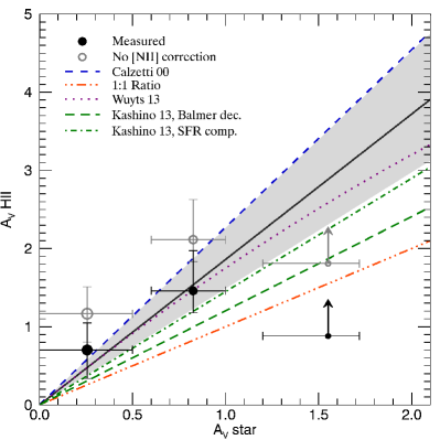
Figure 3.— Weighted average of individual $A_{\mathrm{V\!,\,star}}$ vs. $A_{\mathrm{V\!,\,\textsc{Hii}}}$ measured from the spectra stacked in bins of $A_{\mathrm{V\!,\,star}}$, shown in the top panel of Fig 2, both corrected (black circles) and uncorrected (open grey circles) for [NII] contamination. The size of the data points corresponds to the fraction of the scaled $\mathrm{H\alpha}$+[NII] flux in each bin. Bins without a significant detection ($\geq 2\sigma$) of $\mathrm{H\beta}$ are shown as $2\sigma$ lower limits. The $A_{\mathrm{V\!,\,star}}$ errors shown are the $1\sigma$ scatter within the bins. The black line shows the best-fit line to our [NII] corrected values, which has a slope of 1.86. The fit error is shown with the shaded grey region. The best-fit indicates there is extra attenuation towards emission line regions. The data are consistent with the ratio of $A_{\mathrm{V\!,\,\textsc{Hii}}}$ to $A_{\mathrm{V\!,\,star}}$ from Calzetti et al. (2000) (blue dashed line), Wuyts et al. (2013) (purple dotted line), and both relations found by Kashino et al. (2013) (green long dash, dash-dot lines). The data are inconsistent with the assumption of no extra dust attenuation towards emission line regions (orange dash-dot-dot line).

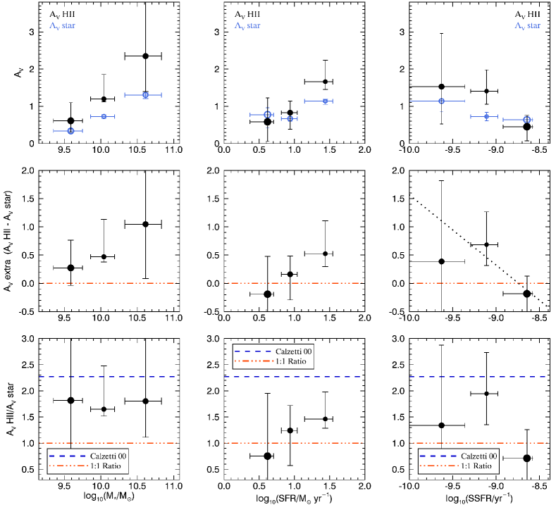
Figure 4.— $A_{\mathrm{V}}$ measurements for bins in $\log M_{*}$, log SFR and log SSFR. The top row shows $A_{\mathrm{V\!,\,star}}$ and $A_{\mathrm{V\!,\,\textsc{Hii}}}$ vs. the binned parameters. The middle row shows the difference between emission and stellar $A_{\mathrm{V}}$ ($A_{\mathrm{V\!,\,extra}}$) vs. the binned parameters. The orange dash-dot-dot line shows the case of no extra attenuation towards star-forming regions. The bottom row shows the ratio of $A_{\mathrm{V\!,\,\textsc{Hii}}}$ to $A_{\mathrm{V\!,\,star}}$ vs. the binned parameters. The blue dashed and orange dash-dot-dot lines in the third row are the ratio between emission $A_{\mathrm{V}}$ and stellar $A_{\mathrm{V}}$ used in Calzetti et al. (2000) and the case of no extra attenuation towards star-forming regions, respectively. The size of the data points is described in Fig. 3. The errors in $\log M_{*}$, log SFR and log SSFR are the $1\sigma$ scatter within the bins. In the right panel the black dotted line shows the best-fit relation of $A_{\mathrm{V\!,\,extra}}=A_{\mathrm{V\!,\,\textsc{Hii}}}-A_{\mathrm{V\!,\,star}}$ vs. log SSFR, with the fit errors shown with the shaded grey region.

3.2. Integrated stellar $A_{\mathrm{V}}$

We first investigate $A_{\mathrm{V\!,\,\textsc{Hii}}}$ in bins of $A_{\mathrm{V\!,\,star}}$, to better constrain the currently contested relationship between the integrated dust content and the dust associated with SF regions for high-redshift galaxies. We choose bins of $A_{\mathrm{V\!,\,star}}$ to probe the full range of integrated stellar dust attenuation in our sample, from low to medium to high attenuation. We stack the spectra in these bins and measure $A_{\mathrm{V\!,\,\textsc{Hii}}}$ on the stack using the relations given in Section 3.1. The results are shown in Figure 3.

We perform a least-squares ratio fit to the data. The best-fit relation, assuming $R_{\mathrm{V}}$ is the same for the stellar continuum and the Hii regions, is

$$A_{\mathrm{V\!,\,\textsc{Hii}}}=1.86_{-0.37}^{+0.40}\ A_{\mathrm{V\!,\,star}},$$ (2)

indicating that on average $A_{\mathrm{V\!,\,\textsc{Hii}}}$ is 1.86 times higher than $A_{\mathrm{V\!,\,star}}$ in star-forming galaxies at $z\sim 1.5$. This is a slightly lower amount of extra attenuation than the ratio of 2.27 which Calzetti et al. (2000) find for low redshift star-forming galaxies, but our data are not statistically different from the Calzetti et al. (2000) relation. The data are inconsistent with the assumption of no extra dust attenuation towards star-forming regions and are inconsistent with a constant value at the $\sigma=1.2,\ 1.7$ levels, respectively.

The data are consistent with the results by Wuyts et al. (2013), who find an average relation between $A_{\mathrm{V\!,\,star}}$ and $A_{\mathrm{V\!,\,extra}}=A_{\mathrm{V\!,\,\textsc{Hii}}}-A_{\mathrm{V\!,\,star}}$ for galaxies at $0.7\leq z\leq 1.5$. Their relation (shown in Figure 3 by the dotted purple line) is the dust attenuation required for agreement between $\mathrm{H\alpha}$ SFRs and UV+IR SFRs, or if there was no IR detection, SED SFRs. Our data are also consistent with the relations Kashino et al. (2013) find by comparing UV and $\mathrm{H\alpha}$ SFR indicators (green dash-dot line) and measured from the Balmer decrement (green long dash line).

We also show the results without correcting the $\mathrm{H\alpha}$ flux for [NII] (open grey circles). These points overestimate the amount of $A_{\mathrm{V\!,\,\textsc{Hii}}}$ relative to $A_{\mathrm{V\!,\,star}}$, demonstrating the necessity of correcting for [NII] when measuring the attenuation of the star-forming regions using grism data.

However, it is important to note that there may be considerable scatter in the $A_{\mathrm{V\!,\,star}}$ and $A_{\mathrm{V\!,\,\textsc{Hii}}}$ values for individual galaxies, so this result only holds on average for a collection of galaxies.

3.3. Stellar mass, SSFR, and SFR

In this section we probe the change in dust properties over bins of stellar mass, SSFR, and SFR. We select bin boundaries for each of these properties to distribute the number of galaxies as equally as possible between the bins.

The left panels of Figure 4 show the results for the stacks in stellar mass, including the measured $A_{\mathrm{V\!,\,\textsc{Hii}}}$ and weighted average $A_{\mathrm{V\!,\,star}}$ (top) and the difference between $A_{\mathrm{V\!,\,\textsc{Hii}}}$ and $A_{\mathrm{V\!,\,star}}$ ($A_{\mathrm{V\!,\,extra}}$, middle) as a function of stellar mass. We also plot the ratio $A_{\mathrm{V\!,\,\textsc{Hii}}}/A_{\mathrm{V\!,\,star}}$ (bottom) to facilitate comparison with previous studies.

We see an increase in both $A_{\mathrm{V\!,\,star}}$ and $A_{\mathrm{V\!,\,\textsc{Hii}}}$ with increasing stellar mass, inconsistent with a constant value at the $\sigma=12,\,1.2$ levels, respectively. The plot of $A_{\mathrm{V\!,\,extra}}$ shows a roughly constant amount of extra attenuation with mass. The data are consistent with a constant value of $A_{\mathrm{V\!,\,extra}}$. The ratio $A_{\mathrm{V\!,\,\textsc{Hii}}}/A_{\mathrm{V\!,\,star}}$ is consistent with the value found by Calzetti et al. (2000) for all mass bins.

The results for stacks in SFR are shown in the center panel of Figure 4. Both $A_{\mathrm{V\!,\,star}}$ and $A_{\mathrm{V\!,\,\textsc{Hii}}}$ show an increase with SFR, at the $\sigma=4.3,\,1.0$ levels, respectively. $A_{\mathrm{V\!,\,extra}}$ is consistent with no trend with SFR. As before, we show the ratio $A_{\mathrm{V\!,\,\textsc{Hii}}}/A_{\mathrm{V\!,\,star}}$ for direct comparison with past work. On average, the ratio is below the value found in Calzetti et al. (2000).

The results for stacks in SSFR are shown in the right panel of Figure 4. Both $A_{\mathrm{V\!,\,star}}$ and $A_{\mathrm{V\!,\,\textsc{Hii}}}$ decrease with increasing SSFR, and are inconsistent with a constant value at the $\sigma=3.2,\,1.2$ levels, respectively.

We also find a slight decreasing trend in $A_{\mathrm{V\!,\,extra}}$ with SSFR, however this trend is not significant as the difference between the data and a constant value is only $\sigma=0.7$. Again, we show the ratio $A_{\mathrm{V\!,\,\textsc{Hii}}}/A_{\mathrm{V\!,\,star}}$ for comparison. Our ratio is consistent with the Calzetti et al. (2000) value for the lowest two SSFR bins, while our ratio for the highest SSFR bin is lower.

Interestingly, $A_{\mathrm{V\!,\,extra}}$ is most strongly correlated with SSFR, rather than stellar mass or SFR. We perform a least-squares linear fit to $A_{\mathrm{V\!,\,extra}}$ vs. log SSFR, using an offset in log SSFR to avoid correlated intercept and slope errors. We find a best-fit relation of

$$A_{\mathrm{V\!,\,extra}}=0.48_{-0.32}^{+0.41}-1.25_{-0.91}^{+0.87}\,\left[\log_{10}(\mathrm{SSFR/yr^{-1}})+9.13\right].$$ (3)

This possible trend could be explained by the two-component dust model, as we discuss in Section 4.1.

4. Discussion

4.1. Physical interpretation

The observed extra attenuation towards emission-line regions, and the decrease in the amount of extra attenuation with increasing SSFR, are consistent with a two-component dust model (e.g., Calzetti et al., 1994; Charlot & Fall, 2000; Granato et al., 2000; Wild et al., 2011). This model assumes there is a diffuse (but possibly clumpy) dust component in the ISM that affects both the older stellar populations and star-forming regions, as well as a component associated with the short-lived stellar birth clouds that only affects the stars within those regions.

For galaxies with the highest SSFRs, the continuum light is dominated by young, massive stars. These massive stars would predominately still reside in the birth clouds. So for the two-component model, both the emission lines and the continuum features would be attenuated by both the birth cloud and the diffuse dust components, resulting in $A_{\mathrm{V\!,\,\textsc{Hii}}}\approx A_{\mathrm{V\!,\,star}}$. Galaxies with lower SSFRs would have a smaller continuum contribution from massive stars, so more of the continuum light would come from stars only attenuated by the diffuse dust, resulting in $A_{\mathrm{V\!,\,\textsc{Hii}}}$ greater than $A_{\mathrm{V\!,\,star}}$. These different cases are illustrated in Figure 5.

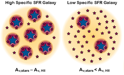
Figure 5.— Illustration of the two-component dust model in galaxies with high (left panel) and low (right panel) specific SFRs. The yellow regions indicate the diffuse dust component in the ISM. The red regions indicate the dust component associated with the short-lived stellar birth clouds. The large blue stars show the young, massive stars which mostly are found in the birth clouds. The small red stars show the less massive stars (both young and old), which are found both within the birth clouds and elsewhere. For galaxies with higher specific SFRs, we expect the continuum light to be dominated by the young, massive stars in the birth clouds, so both the continuum and emission lines are attenuated by both dust components. Galaxies with lower specific SFRs would have a higher contribution to the continuum emission from less massive stars, which generally reside outside the birth clouds and are only attenuated by the diffuse dust component, while the emission lines are still attenuated by both dust components. Thus this leads to larger differences between $A_{\mathrm{V\!,\,star}}$ and $A_{\mathrm{V\!,\,\textsc{Hii}}}$.

We compare our results with those of Wild et al. (2011) for local galaxies. They also find increasing amounts of extra attenuation with decreasing SSFRs, in agreement with the trend we observe. Wild et al. find higher amounts of extra attenuation than we do, but the average SSFRs of their sample are lower than for our sample. The two-component dust model naturally explains this difference, based on the dependence of extra attenuation on SSFR as discussed above. This model may also explain the higher amount of extra attenuation found by Calzetti et al. (2000) if their sample has higher average SSFRs than our sample.

The two-component dust model could also explain the discrepancies found between different high-redshift studies, if the samples consist of galaxies with different ranges in specific SFR. For example, the Kashino et al. (2013) SFR-M_∗ relation implies a higher average SSFR than our sample, and they find a lower amount of extra attenuation. Erb et al. (2006a) find evidence for no extra attenuation, but the average SSFR is higher than for the Kashino et al. sample.

Our explanation for the trend between extra $A_{\mathrm{V}}$ and SSFR was previously mentioned by Wild et al. (2011). They suggest that the trend may alternatively be caused by a decline in diffuse dust with decreasing SSFR. However, we observe that $A_{\mathrm{V\!,\,star}}$ increases slightly with decreasing SSFR, so we do not expect a decline in diffuse dust with decreasing SSFR.

In absolute terms, we find that $A_{\mathrm{V\!,\,\textsc{Hii}}}$ increases with mass and SFR, and decreases with SSFR. As stellar mass and SFR are correlated, the trend of increasing dustiness with SFR and mass could share the same cause. The trend of increasing $A_{\mathrm{V\!,\,star}}$ and $A_{\mathrm{V\!,\,\textsc{Hii}}}$ with decreasing SSFR could also share the same cause, as the SSFR decreases slightly with increasing mass both in the local universe (Brinchmann et al., 2004) and at higher redshifts (Elbaz et al., 2007; Noeske et al., 2007b; Zheng et al., 2007; Damen et al., 2009; Whitaker et al., 2012a). As the trends of $A_{\mathrm{V\!,\,star}}$ and $A_{\mathrm{V\!,\,\textsc{Hii}}}$ with increasing mass are the strongest, it is likely that mass is the key property. This finding may be explained by the fact that more massive star-forming galaxies have higher gas-phase metallicities (Tremonti et al., 2004; Erb et al., 2006a).

We do note that we assume a fixed attenuation law in our work. Recent work (e.g., Wild et al., 2011; Buat et al., 2012; Kriek & Conroy, 2013) shows that the dust attenuation curve varies with SSFR. As the origin of these observed trends are not well understood, and this variation may be the consequence of age-dependent extinction in a two-component dust model, we have decided to use the same dust law for the derivation of the two dust measurements. However, we cannot rule out the possibility that variations in the dust attenuation law may have impacted the trends found in this work.

4.2. Dust attenuation vs. axial ratio

The two-component dust model also predicts a dependence of dust attenuation properties on the axial ratio. Under this model, the amount of dust attenuation from the stellar birth clouds is similar in face-on or edge-on systems, while the longer path length in edge-on systems results in a larger overall $A_{\mathrm{V\!,\,star}}$ and a smaller amount of extra attenuation towards the star-forming regions. Wild et al. (2011) find evidence for the two-component model from the trends of attenuation with axial ratio for objects in the local universe.

The spatially resolved WFC3 images yield excellent axial ratio measurements. However, the axial ratio distribution for our sample is heavily biased towards face-on systems. The more edge-on systems may be dustier, so our selection criteria likely introduce this bias against edge-on systems. It might also be that our sample objects are not disk-like galaxies. Because of sample incompleteness and the small range in axial ratios, we are unable to test the two-component model using the inclinations of the galaxies.

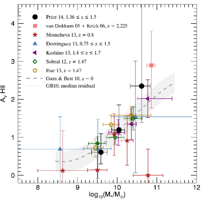
Figure 6.— $A_{\mathrm{V\!,\,\textsc{Hii}}}$ vs. stellar mass comparison between this work and past studies. The filled data (this work; van Dokkum et al., 2005; Momcheva et al., 2013; Domínguez et al., 2013; Kashino et al., 2013) indicate direct measurements of $A_{\mathrm{V\!,\,\textsc{Hii}}}$ using Balmer decrements, while the open data indicate $A_{\mathrm{V\!,\,\textsc{Hii}}}$ measured with a different method that is calibrated using Balmer decrements. The dashed line gives the median relation derived by Garn & Best (2010) using SDSS star-forming galaxies. With the exception of the single object from van Dokkum et al. (2005) (combined with information from Kriek et al., 2006), all other data are the result of stacks (using various stacking schemes, both mean and median) or are mean (Momcheva et al., 2013, combined with stacking) or median values (Garn & Best, 2010; Sobral et al., 2012) from samples.

4.3. Comparison of results for $A_{\mathrm{V\!,\,\textsc{Hii}}}$ vs. stellar mass

A number of past studies have measured Balmer decrements (and often $A_{\mathrm{V\!,\,\textsc{Hii}}}$) versus stellar mass (Kashino et al., 2013; Domínguez et al., 2013; Momcheva et al., 2013; van Dokkum et al., 2005). Other studies have employed different methods of measuring $A_{\mathrm{V\!,\,\textsc{Hii}}}$ versus stellar mass. These methods include comparing $L_{\mathrm{IR}}$ to $L_{\mathrm{H\alpha}}$ as by Ibar et al. 2013, or calibrating [OII]/$\mathrm{H\alpha}$ ratio as an alternate to Balmer decrements as by Sobral et al. 2012. We compare our results with their findings in Figure 6. As necessary, we convert stellar masses derived using a Salpeter or Kroupa IMF to match our assumption of a Chabrier IMF using the relations given in Equations 12 and 13 of Longhetti & Saracco (2009).

The collection of results over a range of redshifts makes it tempting to speculate that there is no redshift evolution in the mass-$A_{\mathrm{V\!,\,\textsc{Hii}}}$ relation. However, the current data are not conclusive. First, there is incompleteness at all masses. Second, the measurements of $A_{\mathrm{V\!,\,\textsc{Hii}}}$ are not necessarily equivalent.

The samples of Domínguez et al. (2013) and Kashino et al. (2013) are similar to ours in redshift and method (stacking) for measuring $A_{\mathrm{V\!,\,\textsc{Hii}}}$. Concerning the work by Domínguez et al. (2013), we first note that their sample contains fewer objects than our sample. Second, we have a broad range of deep photometric coverage for our objects, which reduces the errors in our masses taken from SED modeling. We also do not combine measurements between different grisms, to avoid possible normalization mismatches affecting line fluxes. Compared with Kashino et al. (2013), our sample is larger and on average has slightly lower SSFRs. The trend we observe between $A_{\mathrm{V\!,\,\textsc{Hii}}}$ and SSFR shows that the average $A_{\mathrm{V\!,\,\textsc{Hii}}}$ decreases with increasing SSFR, which explains why their values of $A_{\mathrm{V\!,\,\textsc{Hii}}}$ are lower (though consistent within the errors) than what we measure for similar masses.

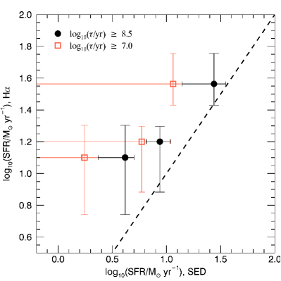
Figure 7.— Comparison between measured $\mathrm{H\alpha}$ SFRs (Kennicutt, 1998) and the SED SFRs. The two sets of SED SFRs differ only in the choice of the minimum star formation e-folding timescale, $\tau$: $\log_{10}(\tau/\mathrm{yr})\geq 7.0$ (open red squares) and $\log_{10}(\tau/\mathrm{yr})\geq 8.5$ (closed black circles). (The dashed black line shows equal $\mathrm{H\alpha}$ SFRs and SED SFRs.) The $\mathrm{H\alpha}$ SFRs agree better with the SED SFRs calculated with the higher $\tau_{min}$, which is similar to previous findings that setting $\tau_{min}\sim 300\ \mathrm{Myr}$ yields the most reasonable SED fits for star-forming galaxies. (See Section 4.4 for a full discussion.) The errors in log SED SFR are the $1\sigma$ scatter within the bins.

4.4. Implications for H$\alpha$ SFR compared with SED SFR

With our measurements of dust attenuation towards Hii regions, we can for the first time directly measure $\mathrm{H\alpha}$ SFRs for a large sample of $z\sim 1.5$ galaxies. We calculate the $\mathrm{H\alpha}$ SFRs using the relation from Kennicutt (1998) converted to a Chabrier (2003) IMF. $\mathrm{H\alpha}$ fluxes are taken from the stacks in SED SFR, and are converted to physical units by comparing the flux of the stack with the weighted average (see Section 2.4) of the individual objects’ $\mathrm{H\alpha}$ fluxes, each corrected for [NII]. The luminosity distance is taken as the weighted average of the individual objects’ luminosity distances. We then use the $\mathrm{H\alpha}$ SFRs to test the much more debated SED SFRs.

The comparison of SFR indicators is shown in Figure 7. The $\mathrm{H\alpha}$ SFRs are compared to the weighted average of SED SFRs derived assuming an exponentially decaying SFH and a minimum e-folding time of $\log_{10}(\tau_{\mathrm{min}}/\mathrm{yr})=8.5$ (shown as filled black circles). For these parameters, the SED SFR values underestimate the $\mathrm{H\alpha}$ SFRs, and are inconsistent at the $\sim 1.5\sigma$ level. However, if a shorter decay time of $\log_{10}(\tau_{\mathrm{min}}/\mathrm{yr})=7$ (open red squares) is adopted, the SED SFRs are low and inconsistent with the $\mathrm{H\alpha}$ SFRs at the $\sim 4\sigma$ level. Thus for our sample, SED SFRs derived with $\log_{10}(\tau_{\mathrm{min}}/\mathrm{yr})=8.5$ are more in line with the $\mathrm{H\alpha}$ SFRs.

This is in general agreement with the work of Wuyts et al. (2011b). They compare UV+IR and SED SFRs and find good agreement between the SFR indicators for $\log_{10}(\tau_{\mathrm{min}}/\mathrm{yr})=8.5$, but when a shorter time of $\log_{10}(\tau_{\mathrm{min}}/\mathrm{yr})=7$ is adopted, they find that the SED SFRs underestimate the true SFRs. Reddy et al. (2012) also compare UV+IR SFRs with SED SFRs. However, instead of using a longer $\tau_{\mathrm{min}}$ for a decreasing SFH, they find the SED SFRs agree with UV+IR SFRs when increasing SFHs are adopted.

The SFR indicators may also differ because they probe different stellar mass ranges, and thus different star formation timescales. The $\mathrm{H\alpha}$ SFRs depend on OB stars, so are averaged over $\sim 10\ \mathrm{Myr}$, while SED SFRs are limited by the discrete nature of SED fitting and depend on the UV flux from O, B and A stars, which live longer. These timescale differences could cause discrepancies for galaxies with episodic or rapidly increasing or decreasing SFHs. However, as we stack multiple objects and thus average over many SFHs, we expect that the timescale differences should not significantly influence the measured SFRs.

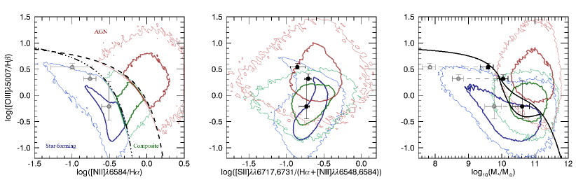
Figure 8.— Left: Traditional BPT (Baldwin et al., 1981) diagram used to identify the ionizing mechanism for optical emission lines. The dashed line is the theoretical limit between star-forming (SF) galaxies and AGN, as derived in Kewley et al. (2001), and the dashed-dot line is the empirical division derived in Kauffmann et al. (2003) for galaxies in the SDSS. The color contours represent SDSS galaxies, divided into three regions according to these dividing lines. The darker, thicker lines enclose 68% of the population, while the lighter, thinner lines enclose 95%. The grey open points represent our stacked spectra (in bins of $M_{*}$), with the [NII]/$\mathrm{H\alpha}$ measurement inferred from the average stellar masses (i.e. not directly measured from the data.) Middle: alternative BPT diagram, using the blended lines observed with the grism. Color contours correspond to the SDSS galaxies in the left panel. The black circles show the measurements from our stacked spectra. This panel illustrates that the combination of blended emission lines does not enable us to discriminate between SF galaxies and AGN. Right: the Mass-Excitation (MEx) diagnostic from Juneau et al. (2011), where the solid lines are the empirical divisions between SF galaxies and AGN, valid for $z<1$ galaxies. Our stacked spectra (black circles) lie on the dividing line between the SF and AGN regions of the diagram. Recently Newman et al. (2014) have shown that high redshift SF galaxies tend to be offset to the right from lower redshift SF galaxies in this diagram. We also apply the empirical correction they derive for $z\sim 2$ galaxies (open grey circles) to better compare our sample to the $z\sim 0$ MEx divisions. (See Section 4.5 for more discussion.)

4.5. AGN contamination

As discussed in Section 2.2, we use a number of methods to reject AGNs from our sample. However, as almost all individual objects do not have sufficient line SNRs, and more importantly we do not have separate [NII] and $\mathrm{H\alpha}$ measurements, we cannot use a BPT (Baldwin et al., 1981) diagram to distinguish whether the line emission originates from star formation or AGN.

After stacking, there is sufficient line SNR to place the binned values in the BPT and alternative diagrams, which we show in Figure 8. These diagrams allow us to assess if there is AGN contamination in the stacks. We use the data from the stacks in stellar mass in these diagrams.

In the left panel, we show the traditional BPT diagram: [NII]/$\mathrm{H\alpha}$ vs. [OIII]/$\mathrm{H\beta}$. Included are the theoretical limit for star-forming (SF) galaxies from Kewley et al. (2001) (dashed line) and the more conservative empirical division between SF galaxies and AGN by Kauffmann et al. (2003) (dashed-dot line), both of which are derived for galaxies at $z\sim 0$. The SDSS DR7 galaxies (Abazajian et al., 2009) are divided into three categories based on these dividing lines: SF galaxies (blue contours), composite (green contours), and AGN (red contours). These same group definitions are used in the alternate BPT diagrams (middle and right of Figure 8). Because we do not measure [NII] directly (instead inferring a value as described in Section 2.4.1), we cannot use the traditional BPT diagram as a post-analysis check. Instead, we show that our inferred [NII]/$\mathrm{H\alpha}$ ratios and the observed [OIII]/$\mathrm{H\beta}$ ratios, shown as open grey circles, are consistent with values for SF galaxies. However, in agreement with other observational (e.g., Shapley et al., 2005; Liu et al., 2008) and theoretical studies (Kewley et al., 2013) of distant galaxies, the data points are moved slightly up (and possibly to the right) in the BPT diagram compared to the average values found in the local star-forming sequence.

An alternate BPT diagram is [SII]/$\mathrm{H\alpha}$ vs. [OIII]/$\mathrm{H\beta}$. However, $\mathrm{H\alpha}$ is not a directly measured quantity, so using the deblended $\mathrm{H\alpha}$ values makes it impossible to detangle the assumptions of the [NII] correction with the possible presence of AGN. Instead, we make an alternate diagram with only directly measured quantities: [SII]/(H$\alpha$+[NII]) vs. [OIII]/$\mathrm{H\beta}$, which we show in the middle panel of Figure 8. There is significant overlap between the different categories of SDSS galaxies, so we are unable to discriminate between SF galaxies and AGN using combinations of blended emission lines.

A final alternate to the BPT diagram, the Mass-Excitation (MEx) diagram (Juneau et al., 2011), is useful as we directly measure the necessary lines ([OIII] and $\mathrm{H\beta}$) and derive stellar mass with SED fitting, which we show in the right panel of Figure 8. The solid black lines are their empirical divisions between SF, composite, and AGN, which are valid up to $z\sim 1$. We include the SDSS categories, using stellar masses from the MPA/JHU value-added catalogs (Kauffmann et al., 2003), to demonstrate that while the separation is not as clean as the traditional BPT diagram, it does separate SF galaxies from AGN in the local universe. Our data are consistent with the SF region as defined by Juneau et al. (2011), though the data do lie on the division boundary. However, work by Newman et al. (2014) at $z\sim 2$ has shown that the low redshift empirical divisions in the MEx diagram incorrectly classify $z\sim 2$ SF galaxies as AGN. They use the shift in the mass-metallicity relation between $z\sim 0$ and 2 to derive a shift to lower mass to bring the high-$z$ values into agreement with the $z\sim 0$ MEx diagram (see Fig. 14 of Newman et al., 2014). This empirical correction (shown as open grey circles in the right panel of Figure 8) shifts our data securely into the SF region of the diagram. These diagnostics demonstrate that there is likely not much AGN contamination to the line emission in our sample.

4.6. [NII] contamination

One of the largest sources of uncertainty in this analysis is our correction for [NII] in our measurement of $\mathrm{H\alpha}$ from the blended H$\alpha$+[NII] line. Figure 3 demonstrates how much our results change when we do not correct for [NII]. We use the relation between [NII]/$\mathrm{H\alpha}$ and stellar mass by Erb et al. (2006a) as a way of detangling the blended lines. We infer the [NII] contribution from the weighted average mass of each stack. Because the two samples have similar masses and SFRs, and are close in redshift, the average sample properties should be fairly similar. Still, the use of this relation may introduce bias into our results.

However, our gas phase metallicities may be different from those of Erb et al. (2006a), due to slight differences in redshift, mass or (S)SFR, which could affect both the slope and scaling of the [NII]/$\mathrm{H\alpha}$ relation. Such trends have been proposed by Mannucci et al. (2010), in the form of the fundamental metallicity relation (FMR). The FMR suggests that metallicity depends on both stellar mass and SFR.

We repeat our analysis using the FMR in conjunction with the Maiolino et al. (2008) [NII]/$\mathrm{H\alpha}$ metallicity calibration as an alternative way of calculating the [NII] correction. This allows us to test whether the trend of $A_{\mathrm{V\!,\,extra}}$ versus SSFR may be due to a variation in [NII]/$\mathrm{H\alpha}$ with SFR. If the FMR is adopted, the $A_{\mathrm{V\!,\,\textsc{Hii}}}$ values are slightly lower than the $A_{\mathrm{V\!,\,\textsc{Hii}}}$ values derived using the Erb et al. (2006a) values, which reduces the strength of the trend of $A_{\mathrm{V\!,\,extra}}$ with SSFR. In this case, the relation we observe between $A_{\mathrm{V\!,\,extra}}$ and SSFR is weaker than the trend presented in Section 3.3, and is consistent with no trend, as the difference is only $\sigma=0.4$. However, the data are still suggestive of a possible decreasing trend of $A_{\mathrm{V\!,\,extra}}$ with SSFR, which would imply the signal is not entirely caused by trends with metallicity.

It is also possible that there is some AGN contamination at the highest masses (Kriek et al., 2007), which would also result in an underestimate of the [NII] fraction. In most cases, our corrected $\mathrm{H\alpha}$ flux would be higher than the true value, leading to an overestimate of $A_{\mathrm{V\!,\,\textsc{Hii}}}$.

We use the mass-[NII]/$\mathrm{H\alpha}$ relation presented in Erb et al. (2006a) for our analysis over the FMR due to uncertainty about metallicity relations at high redshifts. First, the FMR is still not well tested at these redshifts (Cullen et al., 2014). Second, recent work has also questioned whether [NII]/$\mathrm{H\alpha}$ correlates with metallicity at these redshifts (Kulas et al., 2013; Newman et al., 2014). Erb et al. (2006a) present direct measurements of [NII]/$\mathrm{H\alpha}$, which allows us to avoid systematic problems with metallicity calibrations.

4.7. Incompleteness and other systematic uncertainties

One of the strengths of our analysis is that we draw a sample from a non-targeted grism survey, with sample cuts designed to avoid bias as much as possible. However, bias and incompleteness most likely still affect our sample.

The dustiest star-forming galaxies have very attenuated $\mathrm{H\alpha}$ fluxes. Our $\mathrm{H\alpha}$ SNR selection cut, designed to avoid adding noise to our analysis, introduces bias against galaxies with large $A_{\mathrm{V\!,\,\textsc{Hii}}}$. This bias affects the high mass, high SFR end of the sample, as these objects have the largest $A_{\mathrm{V}}$. As lower mass, lower SFR galaxies tend to have lower $\mathrm{H\alpha}$ luminosities, the $\mathrm{H\alpha}$ SNR cut will also exclude objects with the largest $A_{\mathrm{V}}$ values in that mass range.

Our continuum normalization scheme also introduces bias into our analysis. We adopt a normalization scheme to improve the signal of our stack, but the cost is that some objects have much higher scaled $\mathrm{H\alpha}$ fluxes, and thus they dominate our stacks. This biases our results towards those objects with higher $\mathrm{H\alpha}$ equivalent widths in a given bin. Because the line measurements are biased based on the $\mathrm{H\alpha}$ flux, we take the weighted average of the continuum values within a bin to ensure a fair comparison. However, if we instead used a non-weighted average for $A_{\mathrm{V\!,\,star}}$, the $A_{\mathrm{V\!,\,star}}$ vs. $A_{\mathrm{V\!,\,\textsc{Hii}}}$ relationship does not change much.

5. Summary

In this paper, we investigate dust attenuation in $z\sim 1.5$ star-forming galaxies using data from the 3D-HST survey. We measure both the dust towards Hii regions, using Balmer decrements, and the integrated dust properties, using SED modeling. We find that there is extra attenuation towards star-forming regions. On average the total attenuation of these regions, $A_{\mathrm{V\!,\,\textsc{Hii}}}$, is 1.86 times the integrated dust attenuation, $A_{\mathrm{V\!,\,star}}$.

However, the amount of extra attenuation is not the same for all galaxies. We find that the amount of extra attenuation decreases with increasing SSFR, in agreement with the results by Wild et al. (2011) for low-redshift galaxies. Our findings are consistent with the two-component dust model, which assumes there is a diffuse dust component in the ISM and a dust component associated with the short-lived stellar birth clouds. For galaxies with high SSFR, the stellar light will be dominated by continuum emission from the younger stellar population in the birth clouds, resulting in similar attenuation toward the line and continuum emission. For more evolved galaxies, much of the stellar light will only be attenuated by the diffuse ISM, leading to larger discrepancies between the two dust measures. The observed trend of $A_{\mathrm{V\!,\,extra}}$ with SSFR may be affected by uncertainties in the [NII] correction and possible dust attenuation law variations. Future work is necessary to determine what role these effects have on the relation between $A_{\mathrm{V\!,\,extra}}$ and SSFR.

Similar to previous studies (Förster Schreiber et al., 2009; Yoshikawa et al., 2010; Wuyts et al., 2011b, 2013; Kashino et al., 2013), we find less extra attenuation in distant galaxies than is found in the local universe (Calzetti et al., 2000). This effect can also be explained by the two-component model, as lower redshift objects tend to have lower SSFRs than higher redshift galaxies (e.g., Noeske et al., 2007a; Whitaker et al., 2012b; Fumagalli et al., 2012).

We find that both $A_{\mathrm{V\!,\,\textsc{Hii}}}$ and $A_{\mathrm{V\!,\,star}}$ increase with increasing SFR and stellar mass, and decreasing specific SFRs. However, our data are biased against the dustiest objects, which may affect these trends. We also observe there to be little redshift evolution in the $A_{\mathrm{V\!,\,\textsc{Hii}}}$-$M_{*}$ relation, although uncertainties and incompleteness makes it impossible to make a definite claim.

Using the Balmer decrements, we calculate dust-corrected $\mathrm{H\alpha}$ SFRs to test the accuracy of SFRs derived from SED fitting. We find better agreement between the SFR indicators if short SFH decay times are not allowed and the constraint $\log_{10}(\tau/\mathrm{yr})\geq 8.5$ is used. This generally agrees with the results of past studies comparing UV+IR and SED SFRs (Wuyts et al., 2011b) or $\mathrm{H\alpha}$ and SED SFRs (Wuyts et al., 2013). However, even with this constraint the SED SFRs slightly underestimate the $\mathrm{H\alpha}$ SFRs.

We note that our results are slightly impacted by incompleteness and systematic uncertainties. First, we employ SNR cuts on $\mathrm{H\alpha}$ to ensure quality data, which likely results in incompleteness of the dustiest galaxies. Second, to obtain significant $\mathrm{H\beta}$ detections, we stack spectra, and thus our normalization scheme or incorrectly measured integrated properties could impact our measurements.

Most of these issues can be overcome with future observations by a number of new multi-object near infrared spectrographs on 8-10 m class telescopes, among which is MOSFIRE on Keck (McLean et al., 2010). These instruments have higher spectral resolutions, which will avoid blended lines. They will also allow for deeper measurements, which will yield more accurate Balmer decrements of individual objects as well as allowing for investigation of dust to higher $A_{\mathrm{V}}$ limits. Additionally, including rest-frame mid- and far-IR data in future work will ensure more accurate values of $A_{\mathrm{V\!,\,star}}$. Better measurements of $A_{\mathrm{V\!,\,\textsc{Hii}}}$ and $A_{\mathrm{V\!,\,star}}$ are necessary to better constrain the geometric distribution of dust in high redshift galaxies and the effects of the dust-to-star geometry on dust attenuation.

In addition to the stacked spectra (presented in Fig. 2), we also present the average photometry for each bin (see Fig. 9). The photometry covers a much greater wavelength range, so the average photometry allows us to examine the average SED shape outside the limited range covered by the grism spectra. The photometry for each object is first normalized to match the grism normalization (see Section 2.3), and the central wavelength of each filter is de-redshifted using the object’s grism redshift. The data are averaged within each bin, using the normalized fluxes and rest-frame wavelengths. If not all objects in the bin have coverage in a given filter, nearby filters are combined so each averaged photometric point contains at least the same number of measurements as number of objects in the bin, provided the photometry are not too widely separated in wavelength.

For comparison with the average photometry, we also show the average best-fit continuum model and the errors on the best-fit model. Plotting the continuum model and error allows us to examine the error in the amount of Balmer absorption. The average best-fit stellar population model and simulated best-fit models are calculated as described in Section 2.3. The $\pm 3\sigma$ continuum errors are estimated at every wavelength using the simulated continuum models.

The perturbations of the photometry of the individual objects do not lead to large variation in the stacked best-fit models, especially near the Balmer lines. The broad wavelength coverage of the photometry, specifically across the Balmer break, provides reasonably tight constraints on the average amount of Balmer absorption for the stacks.

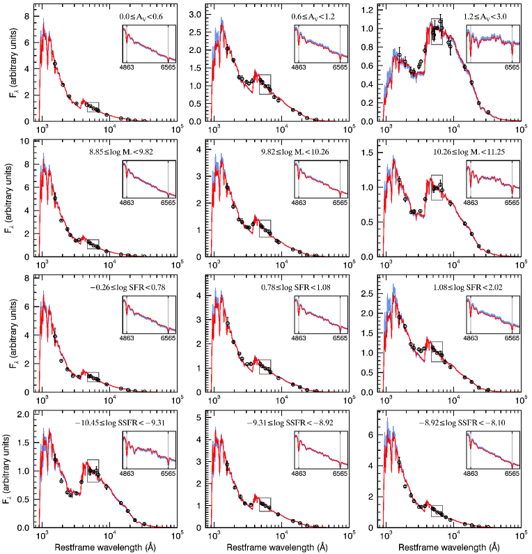
Figure 9.— Binned photometry and stacked best-fit stellar models for bins in stellar $A_{\mathrm{V}}\!$ (top), $\log M_{*}$ (second row), log SFR (third row) and log SSFR (bottom). The photometry is averaged in wavelength bins, and the error is taken to be the error on the mean. The binned photometry is shown by the black circles. The stacked best-fit FAST models are plotted in red. The $3\sigma$ errors in the stacked models are plotted in blue. The insets show the best-fit models (and $3\sigma$ errors) plotted linearly with wavelength near $\mathrm{H\beta}$ and $\mathrm{H\alpha}$ (denoted by left and right vertical grey lines, respectively).

References

- Abazajian et al. (2009) Abazajian, K. N., Adelman-McCarthy, J. K., Agüeros, M. a., et al. 2009, ApJS, 182, 543
- Alexander et al. (2003) Alexander, D. M., Bauer, F. E., Brandt, W. N., et al. 2003, AJ, 126, 539
- Atek et al. (2010) Atek, H., Malkan, M., McCarthy, P., et al. 2010, ApJ, 723, 104
- Baldwin et al. (1981) Baldwin, J. A., Phillips, M. M., & Terlevich, R. 1981, PASP, 93, 5
- Bauer et al. (2002) Bauer, F. E., Alexander, D. M., Brandt, W. N., et al. 2002, AJ, 124, 2351
- Bouwens et al. (2012) Bouwens, R. J., Illingworth, G. D., Oesch, P., et al. 2012, ApJ, 754, 83
- Brammer et al. (2008) Brammer, G. B., van Dokkum, P. G., & Coppi, P. 2008, ApJ, 686, 1503
- Brammer et al. (2012) Brammer, G. B., van Dokkum, P. G., Franx, M., et al. 2012, ApJS, 200, 13
- Brinchmann et al. (2004) Brinchmann, J., Charlot, S., White, S. D. M., et al. 2004, MNRAS, 351, 1151
- Bruzual & Charlot (2003) Bruzual, G., & Charlot, S. 2003, MNRAS, 344, 1000
- Buat et al. (2012) Buat, V., Noll, S., Burgarella, D., et al. 2012, A&A, 545, A141
- Calzetti et al. (2000) Calzetti, D., Armus, L., Bohlin, R. C., et al. 2000, ApJ, 533, 682
- Calzetti et al. (1994) Calzetti, D., Kinney, A. L., & Storchi-Bergmann, T. 1994, ApJ, 429, 582
- Chabrier (2003) Chabrier, G. 2003, PASP, 115, 763
- Charlot & Fall (2000) Charlot, S., & Fall, S. M. 2000, ApJ, 539, 718
- Conroy (2013) Conroy, C. 2013, ARA&A, 51, 393
- Conroy et al. (2010) Conroy, C., Schiminovich, D., & Blanton, M. R. 2010, ApJ, 718, 184
- Cullen et al. (2014) Cullen, F., Cirasuolo, M., McLure, R. J., Dunlop, J. S., & Bowler, R. a. a. 2014, MNRAS, 440, 2300
- Daddi et al. (2007) Daddi, E., Dickinson, M., Morrison, G., et al. 2007, ApJ, 670, 156
- Dale et al. (2012) Dale, D. a., Aniano, G., Engelbracht, C. W., et al. 2012, ApJ, 745, 95
- Damen et al. (2009) Damen, M., Labbé, I., Franx, M., et al. 2009, ApJ, 690, 937
- Domínguez et al. (2013) Domínguez, A., Siana, B., Henry, A. L., et al. 2013, ApJ, 763, 145
- Donley et al. (2012) Donley, J. L., Koekemoer, A. M., Brusa, M., et al. 2012, ApJ, 748, 142
- Draine et al. (2007) Draine, B. T., Dale, D. a., Bendo, G., et al. 2007, ApJ, 663, 866
- Elbaz et al. (2007) Elbaz, D., Daddi, E., Le Borgne, D., et al. 2007, A&A, 468, 33
- Erb et al. (2006a) Erb, D. K., Shapley, A. E., Pettini, M., et al. 2006a, ApJ, 644, 813
- Erb et al. (2006b) Erb, D. K., Steidel, C. C., Shapley, A. E., et al. 2006b, ApJ, 647, 128
- Finkelstein et al. (2012) Finkelstein, S. L., Papovich, C., Salmon, B., et al. 2012, ApJ, 756, 164
- Förster Schreiber et al. (2009) Förster Schreiber, N. M., Genzel, R., Bouché, N., et al. 2009, ApJ, 706, 1364
- Fumagalli et al. (2012) Fumagalli, M., Patel, S. G., Franx, M., et al. 2012, ApJ, 757, L22
- Galliano et al. (2008) Galliano, F., Dwek, E., & Chanial, P. 2008, ApJ, 672, 214
- Garn & Best (2010) Garn, T., & Best, P. N. 2010, MNRAS, 409, 421
- Gonzalez-Perez et al. (2013) Gonzalez-Perez, V., Lacey, C. G., Baugh, C. M., Frenk, C. S., & Wilkins, S. M. 2013, MNRAS, 429, 1609
- Granato et al. (2000) Granato, G. L., Lacey, C. G., Silva, L., et al. 2000, ApJ, 542, 710
- Hainline et al. (2009) Hainline, K. N., Shapley, A. E., Kornei, K. a., et al. 2009, ApJ, 701, 52
- Hathi et al. (2013) Hathi, N. P., Cohen, S. H., Ryan, R. E., et al. 2013, ApJ, 765, 88
- Ibar et al. (2013) Ibar, E., Sobral, D., Best, P. N., et al. 2013, MNRAS, 434, 3218
- Johnson et al. (2007) Johnson, B. D., Schiminovich, D., Seibert, M., et al. 2007, ApJS, 173, 392
- Juneau et al. (2011) Juneau, S., Dickinson, M., Alexander, D. M., & Salim, S. 2011, ApJ, 736, 104
- Kashino et al. (2013) Kashino, D., Silverman, J. D., Rodighiero, G., et al. 2013, ApJ, 777, L8
- Kauffmann et al. (2003) Kauffmann, G., Heckman, T. M., Tremonti, C., et al. 2003, MNRAS, 346, 1055
- Kennicutt (1998) Kennicutt, R. C. 1998, ApJ, 498, 541
- Kewley et al. (2013) Kewley, L. J., Dopita, M. a., Leitherer, C., et al. 2013, ApJ, 774, 100
- Kewley et al. (2001) Kewley, L. J., Dopita, M. A., Sutherland, R. S., Heisler, C. A., & Trevena, J. 2001, ApJ, 556, 121
- Koekemoer et al. (2011) Koekemoer, A. M., Faber, S. M., Ferguson, H. C., et al. 2011, ApJS, 197, 36
- Kong et al. (2004) Kong, X., Charlot, S., Brinchmann, J., & Fall, S. M. 2004, MNRAS, 349, 769
- Kriek & Conroy (2013) Kriek, M., & Conroy, C. 2013, ApJ, 775, L16
- Kriek et al. (2009) Kriek, M., van Dokkum, P. G., Labbé, I., et al. 2009, ApJ, 700, 221
- Kriek et al. (2006) Kriek, M., van Dokkum, P. G., Franx, M., et al. 2006, ApJ, 645, 44
- Kriek et al. (2007) —. 2007, ApJ, 669, 776
- Kulas et al. (2013) Kulas, K. R., McLean, I. S., Shapley, A. E., et al. 2013, ApJ, 774, 130
- Liu et al. (2008) Liu, X., Shapley, A. E., Coil, A. L., Brinchmann, J., & Ma, C. 2008, ApJ, 678, 758
- Longhetti & Saracco (2009) Longhetti, M., & Saracco, P. 2009, MNRAS, 394, 774
- Ly et al. (2012) Ly, C., Malkan, M. A., Kashikawa, N., et al. 2012, ApJ, 747, L16
- Maiolino et al. (2008) Maiolino, R., Nagao, T., Grazian, A., et al. 2008, A&A, 488, 463
- Mancini et al. (2011) Mancini, C., Förster Schreiber, N. M., Renzini, A., et al. 2011, ApJ, 743, 86
- Mannucci et al. (2010) Mannucci, F., Cresci, G., Maiolino, R., Marconi, A., & Gnerucci, A. 2010, MNRAS, 408, 2115
- McLean et al. (2010) McLean, I. S., Steidel, C. C., Epps, H., et al. 2010, in Proceedings of SPIE, ed. I. S. McLean, S. K. Ramsay, & H. Takami, Vol. 7735, 77351E–77351E–12
- Mendez et al. (2013) Mendez, A. J., Coil, A. L., Aird, J., et al. 2013, ApJ, 770, 40
- Meurer et al. (1999) Meurer, G. R., Heckman, T. M., & Calzetti, D. 1999, ApJ, 521, 64
- Momcheva et al. (2013) Momcheva, I. G., Lee, J. C., Ly, C., et al. 2013, AJ, 145, 47
- Nelson et al. (2013) Nelson, E. J., van Dokkum, P. G., Momcheva, I., et al. 2013, ApJ, 763, L16
- Newman et al. (2014) Newman, S. F., Buschkamp, P., Genzel, R., et al. 2014, ApJ, 781, 21
- Noeske et al. (2007a) Noeske, K. G., Faber, S. M., Weiner, B. J., et al. 2007a, ApJ, 660, L47
- Noeske et al. (2007b) Noeske, K. G., Weiner, B. J., Faber, S. M., et al. 2007b, ApJ, 660, L43
- Osterbrock & Ferland (2006) Osterbrock, D. E., & Ferland, G. J. 2006, Astrophysics of gaseous nebulae and active galactic nuclei, 2nd edn. (Sausalito, CA: University Science Books)
- Reddy et al. (2010) Reddy, N. A., Erb, D. K., Pettini, M., Steidel, C. C., & Shapley, A. E. 2010, ApJ, 712, 1070
- Reddy et al. (2012) Reddy, N. A., Pettini, M., Steidel, C. C., et al. 2012, ApJ, 754, 25
- Reddy et al. (2006) Reddy, N. A., Steidel, C. C., Fadda, D., et al. 2006, ApJ, 644, 792
- Rosario et al. (2013) Rosario, D. J., Mozena, M., Wuyts, S., et al. 2013, ApJ, 763, 59
- Savaglio et al. (2005) Savaglio, S., Glazebrook, K., Le Borgne, D., et al. 2005, ApJ, 635, 260
- Shapley (2011) Shapley, A. E. 2011, ARA&A, 49, 525
- Shapley et al. (2005) Shapley, A. E., Coil, A. L., Ma, C., & Bundy, K. 2005, ApJ, 635, 1006
- Skelton et al. (2014) Skelton, R. E., Whitaker, K. E., Momcheva, I. G., et al. 2014, ApJS, submitted, (arXiv:1403.3689)
- Sobral et al. (2012) Sobral, D., Best, P. N., Matsuda, Y., et al. 2012, MNRAS, 420, 1926
- Teplitz et al. (2000) Teplitz, H. I., McLean, I. S., Becklin, E. E., et al. 2000, ApJ, 533, L65
- Tremonti et al. (2004) Tremonti, C. A., Heckman, T. M., Kauffmann, G., et al. 2004, ApJ, 613, 898
- van Dokkum et al. (2005) van Dokkum, P. G., Kriek, M., Rodgers, B., Franx, M., & Puxley, P. 2005, ApJ, 622, L13
- van Dokkum et al. (2011) van Dokkum, P. G., Brammer, G., Fumagalli, M., et al. 2011, ApJ, 743, L15
- Villar et al. (2008) Villar, V., Gallego, J., Pérez‐González, P. G., et al. 2008, ApJ, 677, 169
- Watson et al. (2009) Watson, M. G., Schröder, A. C., Fyfe, D., et al. 2009, A&A, 493, 339
- Whitaker et al. (2012a) Whitaker, K. E., Kriek, M., van Dokkum, P. G., et al. 2012a, ApJ, 745, 179
- Whitaker et al. (2012b) Whitaker, K. E., van Dokkum, P. G., Brammer, G., & Franx, M. 2012b, ApJ, 754, L29
- Wild et al. (2011) Wild, V., Charlot, S., Brinchmann, J., et al. 2011, MNRAS, 417, 1760
- Wilkins et al. (2011) Wilkins, S. M., Bunker, A. J., Stanway, E., Lorenzoni, S., & Caruana, J. 2011, MNRAS, 417, 717
- Wuyts et al. (2011a) Wuyts, S., Förster Schreiber, N. M., van der Wel, A., et al. 2011a, ApJ, 742, 96
- Wuyts et al. (2011b) Wuyts, S., Förster Schreiber, N. M., Lutz, D., et al. 2011b, ApJ, 738, 106
- Wuyts et al. (2012) Wuyts, S., Förster Schreiber, N. M., Genzel, R., et al. 2012, ApJ, 753
- Wuyts et al. (2013) Wuyts, S., Förster Schreiber, N. M., Nelson, E. J., et al. 2013, ApJ, 779, 135
- Xue et al. (2011) Xue, Y. Q., Luo, B., Brandt, W. N., et al. 2011, ApJS, 195, 10
- Yoshikawa et al. (2010) Yoshikawa, T., Akiyama, M., Kajisawa, M., et al. 2010, ApJ, 718, 112
- Zheng et al. (2007) Zheng, X. Z., Bell, E. F., Papovich, C., et al. 2007, ApJ, 661, L41