High redshift signatures in the 21 cm forest due to cosmic string wakes

Abstract

Cosmic strings induce minihalo formation in the early universe. The resultant minihalos cluster in string wakes and create a “21 cm forest” against the cosmic microwave background (CMB) spectrum. Such a 21 cm forest can contribute to angular fluctuations of redshifted 21 cm signals integrated along the line of sight. We calculate the root-mean-square amplitude of the 21 cm fluctuations due to strings and show that these fluctuations can dominate signals from minihalos due to primordial density fluctuations at high redshift ($z\gtrsim 10$), even if the string tension is below the current upper bound, $G\mu<1.5\times 10^{-7}$. Our results also predict that the Square Kilometre Array (SKA) can potentially detect the 21 cm fluctuations due to strings with $G\mu\approx 7.5\times 10^{-8}$ for the single frequency band case and $4.0\times 10^{-8}$ for the multi-frequency band case.

1 Introduction

Cosmic strings are linear topological defects that could form at phase transitions in the early universe [1] (see refs. [2, 3] for reviews). Probing the observational signatures of cosmic strings therefore allows us to constrain high energy particle physics and the early universe.

Since cosmic strings have energies which depend on the energy scale of early phase transitions, they can gravitationally induce various observational phenomena. In particular, cosmic strings can produce density fluctuations [4, 5] and serve as seeds for the formation of large-scale structures and galaxies [6]. Recent cosmological observations have shown that the cosmic string contribution to the density fluctuations and large-scale structure formation is sub-dominant [7, 8, 9]. Constraints on the gravitational interaction of cosmic strings are given in terms of $G\mu$ where $G$ is Newton’s constant and $\mu$ is the string tension. A current strong constraint on $G\mu$ is obtained from CMB anisotropy observations. Planck data provide the limit, $G\mu<1.5\times 10^{-7}$ [10]. However, cosmic strings below the current limit still have the potential to induce early structure formation and early reionization [11, 12, 13, 14, 15]. In particular, moving long cosmic strings can develop virialized planar objects called ’string wakes’ after the epoch of radiation-matter equality.

Observations of redshifted 21 cm lines from neutral hydrogen are expected to be good probes for the signatures of structure formation due to cosmic strings. The intensity of redshifted 21 cm lines depends on the number density and temperature of neutral hydrogen. Therefore, the measurement of redshifted 21 cm lines enables us to access the evolution of structure formation and the thermal state of the intergalactic medium through the epoch of reionization ($8\lesssim z\lesssim 20$) to the dark ages ($z\gtrsim 20$) (for reviews, see refs. [16, 17]). Currently, there are several ongoing and future projects for measuring highly redshifted 21 cm lines; MWA, LOFAR, GMRT, SKA and Omniscope [18]. Several papers have investigated redshifted 21 cm signatures from string wakes produced by long strings [19, 20, 21, 22] and filaments created by string loops [23, 24]. However, since planar and filamentary objects are gravitationally unstable, string wakes and filaments can fragment to “minihalos” whose virial temperature is below $10^{4}~{}$K [13, 15]. The minihalos due to string wakes can dominate nonlinear structures at $z\gtrsim 15$, even if $G\mu$ is set to the current upper bound.

Minihalos are virialized nonlinear objects whose masses span the range from less than $10^{4}~{}M_{\odot}$ to $10^{8}~{}M_{\odot}$. Therefore detection of minihalos is an important channel for accessing information about small-scale density fluctuations. Since the virial temperature of minihalos is generally below the threshold for atomic hydrogen line cooling, and in the lower mass range even below the threshold for molecular hydrogen cooling, they cannot further collapse to form stars. Accordingly, it is difficult to observe minihalos directly because they are not accompanied by luminous objects. However, the hydrogen density and the temperature in minihalos is high enough to contribute to deviations of the population of the hyperfine levels in neutral hydrogen from the background values. Therefore, minihalos can in principle be detectable as sources of redshifted 21 cm lines [25, 26, 27, 28].

In this paper, we study redshifted 21 cm signals from minihalos due to cosmic strings. Such minihalos cluster in cosmic string wakes and create a “21 cm forest” that is detectable against the CMB spectrum. Since wakes are distributed discretely, the 21 cm forest in wakes contributes to the angular fluctuations of 21 cm signals. Generally, clustering (or non-Gaussianity) of minihalo distributions can enhance the fluctuations of 21 cm signals integrated along the line of sight [29]. Clustering depends on the fragmentation of wakes to minihalos. Adopting a simple analytic model, we calculate the fluctuations of 21 cm signals due to string wakes.

This paper is organized as follows. In section 2, we briefly review the formation of minihalos due to cosmic strings. In section 3, we discuss the 21 cm signal from a single minihalo. In section 4, we calculate observational predictions of rms fluctuations of the redshifted 21 cm lines from minihalos due to cosmic strings. We also discuss the detectability of the fluctuation signals by SKA. We conclude in section 5. Throughout the paper, we are using natural units, $\hbar=c=1$. We also assume a flat $\Lambda$CDM model with cosmological parameters, $h=0.7$, $h^{2}\Omega_{b}=0.023$ and $h^{2}\Omega_{c}=0.115$.

2 Minihalo formation in cosmic string wakes

Due to the geometrical effects of a moving long string, matter accretes onto a planar wake formed behind this string. The wake grows by matter accretion and finally becomes a planar virialized object. However, since a planar object is unstable by virtue of its own self-gravity, the wake fragments into minihalos. In this section, following ref. [15], we briefly review minihalo formation in cosmic string wakes.

2.1 Cosmic string wakes

The geometry around a straight cosmic string is conical with the deficit angle, $\alpha=8\pi\mu$ [30]. Due to this geometrical effect, a moving long string with relativistic velocity $v_{s}$ gives matter a kick velocity in the direction of the plane swept out by the string,

$$v_{k}=4\pi G\mu v_{s}\gamma_{s},$$ (2.1)

where $\gamma_{s}$ is the Lorentz factor of $v_{s}$. Accordingly, the two streams of matter overlap in the string wake and produce an overdense region. After radiation-matter equality, the wake evolves by gravitational instability and finally collapses to a virialized planar object [6].

The evolution of a string wake has been studied by using the Zel’dovich approximation [31, 2]. We consider a matter particle at an initial comoving distance $x$ on a wake. At the initial time $t_{i}$, the matter particle obtains a kick velocity $v_{k}$. The trajectory of this particle can be written as

$$r(x,t)=a(t)(x+\psi(x,t)),$$ (2.2)

where $\psi$ is the comoving displacement (for simplicity, we assume that the scale factor is normalized as $a(t_{i})=1$ in this section). In the Zel’dvich approximation, the evolution of $\psi$ in the matter dominated epoch is given by

$$\ddot{\psi}+\frac{4}{3t}\dot{\psi}-\frac{2}{3t^{2}}\psi=0,$$ (2.3)

with the initial condition, $\psi(x,t_{i})=0$ and $\dot{\psi}(x,t_{i})=-v_{k}\epsilon(x)$ where $\epsilon(x)=1$ for $x>0$ and $\epsilon(x)=-1$ for $x<0$. In eq. (2.3), the dot denotes the time-derivative. The solution of eq. (2.3) can be written in the limit of $t\gg t_{i}$ as

$$\psi(t)\approx-\frac{3v_{k}t_{i}}{5}\left(\frac{t}{t_{i}}\right)^{2/3}.$$ (2.4)

The turn-around comoving surface $x_{\rm ta}$ at time $t$, which is the distance of a matter particle decoupling from the Hubble expansion, is obtained by the condition $\dot{r}(x_{\rm ta},t)=0$. This condition is equivalent with $x_{\rm ta}(t)+2\psi(x_{\rm ta},t)=0$. The turn-around condition provides the turn-around comoving surface as

$$x_{\rm ta}(t,t_{i})=\pm\frac{6}{5}v_{k}t_{i}\left(\frac{t}{t_{i}}\right)^{2/3}.$$ (2.5)

From the turn-around condition, $x_{\rm ta}(t)+2\psi(x_{\rm ta},t)=0$, the wake width, which is the physical distance from the wake’s center to the turnaround surface, is

$$w(t,t_{i})=|r(x_{\rm ta},t)|=\frac{1}{2}a(t)x_{\rm ta}(t,t_{i}).$$ (2.6)

After turn-around, accretion proceeds, and accreted matter is finally virialized. We assume that accreted matter reaches a virialized state when its radius shrinks by a factor of 2 from that at turnaround. This assumption for virialization gives the relation between the virialization time $t_{c}$ and the turnaround time $t_{\rm ta}$; $t_{c}=(1+1/\sqrt{2})^{3/2}t_{\rm ta}$.

Due to virialization, the accreted matter is thermalized in a wake and heated to $T_{w}$ provided by

$$T_{w}=\frac{\mu_{m}m_{p}}{3k_{B}}v_{c}^{2},$$ (2.7)

where $k_{B}$ is the Boltzmann constant, $m_{p}$ is the proton mass, $\mu_{m}$ is the mean molecular weight, and $v_{c}$ is the velocity of accreted matter at the time $t_{c}$. With the relation between $t_{\rm ta}$ and $t_{c}$, the thermalized temperature is evaluated as

$$T_{w}\approx 0.7~{}(v_{s}\gamma_{s})^{2}\left(\frac{G\mu}{10^{-7}}\right)^{2}\left(\frac{z_{i}+1}{z+1}\right)~{}[{\rm K}],$$ (2.8)

where $z$ and $z_{i}$ correspond to the redshifts at $t$ and $t_{i}$, respectively.

2.2 Minihalo formation

The size of a cosmic string wake depends on the initial time $t_{i}$ at which a string starts to produce the wake. Therefore, we need to model the cosmic string network. The string network is likely to evolve toward a scaling solution at which the string distribution is statistically independent of time if string lengths are scaled to the Hubble radius. For a representation of the cosmic string network, we adopt an analytical toy model given in refs. [20, 15].

Cosmic strings can produce wakes after the time of matter-radiation equality, $t_{eq}$. We divide time from the time $t_{eq}$ to the present time $t_{0}$ into Hubble time steps. We label the Hubble time steps as $t_{1}=t_{eq},~{}t_{2}=2t_{eq},...,t_{m}=2^{m-1}t_{eq}$. In each time step, we assume $N_{s}$ long strings per Hubble volume. Each string has a length $\gamma t$ ($\gamma\lesssim 1$) and a velocity $v_{s}$ in a random direction. We also assume that the string networks are uncorrelated between different Hubble time steps.

Now we consider a long string laid down at time $t_{m}$. We assume that the string makes a virialized wake with the initial dimension $\gamma t_{m}\times v_{s}\gamma_{s}t_{m}\times w_{m}(z_{m})$ where $w_{m}(z)=w(t,t_{m})$ and $z_{m}$ denotes the redshift at time $t_{m}$. A wake evolves with time. The planar dimension $\gamma t_{m}\times v_{s}\gamma_{s}t_{m}$ grows due to the Hubble expansion, while the growth of the wake width $w_{m}$ follows eq. (2.6). Therefore, the volume of the wake at a redshift $z$,

$$V_{\rm wake}(z,z_{m})=(\gamma t_{m}\times v_{s}\gamma_{s}t_{m}\times w_{m}(z))\left(\frac{z_{m}+1}{z+1}\right)^{2}.$$ (2.9)

The mass of the wake at $z$ is given by

$$M_{\rm wake}(z,z_{m})=4\rho_{b}(z)V_{\rm wake}(z,z_{m}),$$ (2.10)

where $\rho_{b}(z)$ is the background density at $z$ and, in a factor of four, a factor of two comes from eq. (2.6) and the another of two is due to the fact that the virial radius is half of the wake width.

A planar wake is gravitationally unstable. A wake fragments into filamentary structures and, finally, these filaments break into beads. The length scale of the fastest growing mode is roughly $2\pi w(t)$ in both fragmentations to filaments and to beads [32, 33, 13]. Therefore, we assume that a string wake fragments to beads with radius $w_{m}(z)$. Since the density in a virialized wake is four times larger than the background one, the mass of a fragmented bead is given by

$$M_{m}(z)=\frac{16\pi}{3}\rho_{b}(z)w_{m}^{3}(z).$$ (2.11)

Finally, the resulting beads are virialized to form quasi-spherical halos. The virial temperature of a virialized halo can be obtained from

$$T_{\rm vir}=\frac{\mu_{m}}{3}\frac{m_{p}}{k_{B}}v_{\rm vir}^{2},$$ (2.12)

where $v_{\rm vir}$ is the gas velocity of the halo. Assuming that the virialization is accomplished at the half-radius of the wake $w$, $r_{\rm vir}=\omega/2$, we can obtain $v_{\rm vir}$ by solving equations for the virial relation,

$$2\frac{1}{2}v_{\rm vir}^{2}=\frac{3}{5}\frac{GM}{r_{\rm vir}},$$ (2.13)

and the energy conservation between a pre-virialized bead and a virialized halo,

$$\frac{1}{2}v_{\rm b}^{2}-\frac{3}{5}\frac{GM}{w}=\frac{1}{2}v_{\rm vir}^{2}-\frac{3}{5}\frac{GM}{r_{\rm vir}},$$ (2.14)

where $r_{\rm vir}$ is the radius of a virialized halo and $v_{b}$ is the thermal velocity in a bead. Since the fragmentation does not change the thermal energy significantly, we assume that the velocity $v_{b}$ corresponds to the wake temperature $T_{w}$ given in eq. (2.8).

We plot the redshift evolutions of halo mass and virial temperature in wakes produced at different $z_{m}$ in figure 1. In the figure, we take $G\mu=10^{-7}$. We also use $v_{s}=0.5$ and $\gamma=1$. As the redshift decreases, both values increase. The redshift dependences of halo mass and virial temperature are roughly $z^{-3}$ and $z^{-1}$. Halos due to string wakes have lower density and cooler virial temperature than in the standard $\Lambda$CDM model (cf. $T_{\rm vir}\approx 700(M/10^{6}M_{\odot})^{2/3}(z/10)$ K [34]). As shown in the right panel of figure 1, the virial temperature of halos in wakes is below 200 K even at $z=5$. The virial temperature of the halos is not high enough for atomic cooling ($T_{\rm vir}\gtrsim 10^{4}$ K) nor even for hydrogen molecular cooling ($T_{\rm vir}\gtrsim 200$ K). Therefore, these “minihalos” cannot contribute to star and galaxy formations in the early universe.

For reference, we plot the CMB temperature as the thin line in the right panel of figure 1. At high redshifts, the virial temperature of halos is lower than the CMB temperature. Therefore, the 21 cm signals of minihalos are expected as absorption signals against the CMB. On the other hand, the virial temperature of halos in old wakes at lower redshifts becomes larger than the CMB temperature. The signals from such minihalos are emission signals. We discuss these in more detail in the following section.

Since we assume that the virial radius is a half of the bead radius, $w(z)/2$, the typical density of minihalos is eight times larger than the one of a virialized planar wake. Therefore, in terms of the background matter density $\rho_{b}$, the typical density of the minihalos can be expressed by $\overline{\rho}_{\rm vir}=32\rho_{b}$.

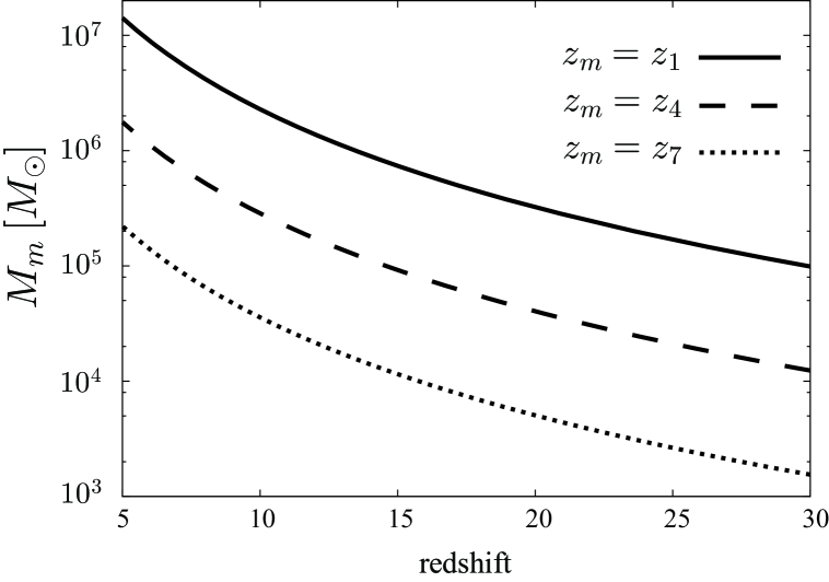
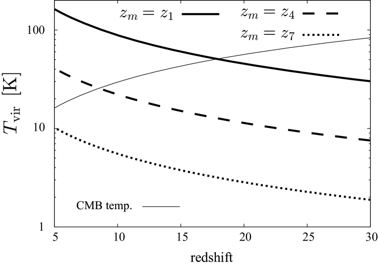
Figure 1: Redshift evolutions of halo mass (left panel) and halo virial temperature (right panel) in a string wake. We set $G\mu=10^{-7}$. In both panels, different types of lines represent different $z_{m}$ at which a wake formed. The solid, dashed and dotted lines are for $z_{m}=z_{1}\sim 3000$, $z_{4}\sim 1000$ and $z_{7}\sim 300$, respectively. In the right panel, the thin line represents the CMB temperature.

3 Redshifted 21 cm lines from a minihalo

Although a minihalo cannot produce stars and galaxies, the density of neutral hydrogen becomes denser and the gas temperature is heated higher than the background values. As a result, the spin temperature of a minihalo is decoupled from the CMB temperature and is different from the background spin temperature. Therefore, a single minihalo can generate an observable 21 cm line signal.

The 21 cm signal from a minihalo depends on the profiles of the hydrogen density and temperature in a minihalo. The shock thermalization at the virialization of a minihalo makes the minihalo isothermal at $T_{\rm vir}$. For simplicity, we assume that the baryon density of a minihalo inside the virial radius is also uniform due to the shock, $\rho_{\rm vir}=32\rho_{b}$.

The 21 cm signal from a single halo is observed as an emission or absorption signal against the CMB. Therefore, it is useful to express the observed 21 cm line flux from a minihalo per unit frequency relative to the CMB photon flux [25],

$$\frac{d\delta F}{d\nu}=2{\nu^{2}}{\delta T_{b}}\Delta\Omega_{\rm halo},$$ (3.1)

where $\delta F$ is the differential total flux from the CMB photon flux, $\Delta\Omega_{\rm halo}$ is the solid angle subtended by the minihalo, $\Delta\Omega_{\rm halo}=\pi R_{\rm vir}^{2}/D_{A}^{2}$ with the comoving minihalo radius, $R_{\rm vir}=(1+z)r_{\rm vir}$, and the comoving angular diameter distance $D_{A}$ to $z$. In eq. (3.1), ${\delta T_{b}}$ is the redshifted differential brightness temperature averaged over the minihalo cross-section, $A=\pi R_{\rm vir}^{2}$,

$${\delta T_{b}}=\frac{1}{1+z}\left(\frac{\int dA~{}T_{b}(\alpha)}{A}-T_{\rm CMB}(z)\right),$$ (3.2)

where $T_{b}(\alpha)$ is the brightness temperature along a line of sight through the minihalo and a function of impact parameter $\alpha$ (in unit of $R_{\rm vir}$) from the centre of the minihalo.

We obtain $T_{b}(\alpha)$ from the equation,

$$T_{b}(\alpha)=T_{\rm CMB}(z)e^{-\tau(\alpha)}+\int_{0}^{\tau(\alpha)}T_{S}e^{-\tau^{\prime}}d\tau^{\prime}.$$ (3.3)

where $\tau$ is the 21 cm optical depth of neutral hydrogen to photons along a line of sight with impact parameter $\alpha$ and $T_{S}$ is the spin temperature.

The 21 cm optical depth with $\alpha$ at frequency $\nu$ is provided by [26]

$$\tau(\nu)=\frac{3A_{10}T_{*}}{32\pi\nu_{*}^{2}}\int_{-\infty}^{\infty}\frac{n_{\rm HI}(\ell)\phi(\nu_{\rm em})}{T_{S}(\ell)}dR^{\prime},$$ (3.4)

where $A_{10}=2.85\times 10^{-15}~{}{\rm s}^{-1}$ is the Einstein $A$-coefficient for the 21 cm transition, $n_{\rm HI}$ is the number density of neutral hydrogen in the minihalo, $\phi(\nu)$ is the normalized line profile, $\nu_{\rm em}$ is $\nu_{\rm em}=(1+z)\nu$, $\ell$ is a radial comoving distance given by $\ell^{2}=R^{\prime 2}+(\alpha R_{\rm vir})^{2}$, and the subscript $*$ denotes the values corresponding to $21~{}$cm. Since gas inside the minihalo is thermalized at $T_{\rm vir}$, the line profile is broadened by the thermal Doppler shift,

$$\phi(\nu_{\rm em})=(\Delta\nu_{D}\sqrt{\pi})^{-1}\exp\left(-\frac{(\nu_{\rm em}-\nu_{*})^{2}}{\Delta\nu_{D}^{2}}\right),$$ (3.5)

where $\Delta\nu_{D}=\nu_{*}\sqrt{2k_{B}T_{\rm vir}/m_{\rm H}}$ with hydrogen mass $m_{\rm H}$.

The spin temperature $T_{S}$ is determined by the balance between CMB photon absorption, collision between atoms and scattering off Ly$\alpha$ photons [35],

$${T_{S}}=\frac{T_{\rm CMB}+y_{c}T_{\rm vir}+y_{\alpha}T_{\alpha}}{1+y_{c}+y_{\alpha}},$$ (3.6)

where $y_{c}$ and $y_{\alpha}$ are the collisional and Ly$\alpha$ coupling constants. Throughout this paper, we neglect the Ly$\alpha$ coupling terms, because we are interested in high redshifts where Ly$\alpha$ photon sources (stars and galaxies) do not form efficiently. For $y_{c}$, we use the values in ref. [36].

Since the 21 cm signals are either line emission or absorption, the total (integrated) differential flux from a minihalo is obtained by multiplying the flux at $\nu=(1+z)\nu_{*}$ by a redshifted effective line width $\Delta\nu_{\rm eff}$ [25],

$$\delta F={2\nu^{2}}{\delta T_{b}}\Delta\Omega_{\rm halo}{\Delta\nu_{\rm eff}.}$$ (3.7)

For the case of a thermal Doppler shift, the effective line width is given by $\Delta\nu_{\rm eff}=\sqrt{\pi}{\Delta\nu_{D}}/(1+z)$.

Since we assume that the gas density and temperature are homogeneous in a minihalo, the spin temperature of the minihalo is also homogeneous. According to eq. (3.3) in the limit of $\tau\ll 1$, the differential 21 cm flux from the minihalo is proportional to ${T_{S}}-T_{\rm CMB}$. We plot the redshift evolution of this value for wakes with different $z_{m}$ in figure 2. With the gas temperature increasing, the collision coupling becomes large and the spin temperature is more efficiently dragged to the gas temperature from the CMB temperature. The virial temperature of minihalos is larger in old wakes (small $m$ label) than in young wakes, as shown in figure 1. Therefore, the deviation of the spin temperature from the CMB temperature is larger in minihalos inside wakes with small $m$ label.

Figure 2 also shows that the difference between ${T_{S}}$ and $T_{\rm CMB}$ becomes large, as the redshift increases. This is because the virial temperature is low at high redshifts as shown in figure 1. The collisional coupling at high redshifts is efficient due to the redshift dependence of the density, even though the virial temperature decreases. The spin temperature is dragged down to the low virial temperature and the difference from the CMB temperature is enhanced.

As wakes grow, the virial temperature of minihalos increases and, finally, it becomes larger than the CMB temperature as shown in figure 1. At this time, the 21 cm signal changes from absorption lines (${T_{S}}-T_{\rm CMB}<0$) to emission lines (${T_{S}}-T_{\rm CMB}>0$). We can see this transition for $z_{m}=z_{1}$ or $z_{4}$ in figure 2 where the absorption and emission signals are represented as thick and thin lines, respectively. The redshifts at which the signal transitions occur correspond to those at which each virial temperature exceeds the CMB temperature in figure 1.

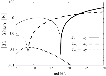
Figure 2: Redshift evolution of the difference between spin temperature and CMB temperature in halos inside a string wake. We set $G\mu=10^{-7}$. The meaning of the line types is the same as in figure 1. The thin lines at lower redshifts for $z_{m}=z_{1}$ and $z_{4}$ represent positive values (i.e. emission signals), while the thick lines denote negative values (i.e. absorption signals).

4 Fluctuations due to the 21 cm forest in cosmic string wakes

Minihalos cluster inside a cosmic string wake. These minihalos create a “21 cm forest” of emission or absorption lines against the CMB spectrum, when CMB photons pass through a string wakes. Therefore, the distribution of a 21 cm forest depends on that of the string wakes and it can contribute to the angular fluctuations of redshifted 21 cm signals. In planning observations by a radio array, the key observable value is the root-mean-square (rms) fluctuations of redshifted 21 cm signals integrated along the line of sight with observation frequency bandwidth. In this section, we evaluate the rms fluctuations, assuming an observation at a mean frequency $\nu_{\rm obs}$ where the survey volume is pixelized with frequency bandwidth $\Delta\nu$ and beam size $\Delta\theta$ in the longitudinal and transverse directions, respectively

We consider a spherical redshift shell at $z_{\rm obs}$, which satisfies $\nu_{\rm obs}=(1+z_{\rm obs})\nu_{*}$, with width $\Delta z$ corresponding to the observation frequency bandwidth $\Delta\nu$. We divide the shell into cells whose angular size equals the beam size $\Delta\theta$ of the observation. We begin by evaluating the fraction of cells where a wake is produced by strings laid down at time $t_{m}$.

When we consider strings with number density $n_{s}$ and velocity $v_{s}$, the number of strings that cross this shell is given by [20]

$$N_{m}=4\pi r_{m}^{2}n_{s}v_{s}\cos\theta_{s}/H_{m}=4\pi r_{m}^{2}N_{s}v_{s}\cos\theta_{s}H_{m}^{2},$$ (4.1)

where $r_{m}$ is the physical radius of the shell at $z_{m}$, $H_{m}$ is the Hubble parameter at $z_{m}$ and $\theta_{s}$ is the angle between the direction of velocity and the normal vector to the shell. For simply, we assume the averaged angle is $\langle\cos^{2}\theta_{s}\rangle=1/2$. At the last equality sign, we rewrite $N_{m}$ in terms of the number of strings per Hubble volume, $N_{s}$, for convenience. The number $N_{m}$ corresponds to the number of wakes on the shell.

For simplicity, we consider the case where a string vertically crosses the shell sphere ($\cos\theta_{s}=1$). The cross section dimension of the string crossing the sphere is $\gamma t_{m}\times w_{m}(z_{m})$ at $z_{m}$. As time increases, the wake grows and the cross section dimension reaches $\gamma t_{m}(1+z_{m})/(1+z_{\rm obs})\times w_{m}(z_{\rm obs})$ at $z_{\rm obs}$. Since the angular size of $w_{m}(z_{\rm obs})$ much less than $\Delta\theta$, the wake at $z_{\rm obs}$ stretches $\gamma t_{m}(1+z_{m})/(1+z_{\rm obs})/\Delta d$ cells on the sphere where $\Delta d$ corresponds to the physical scale of $\Delta\theta$ at $z_{\rm obs}$. Therefore, the fraction of cells at which we can find a wake produced by strings laid down at time $t_{m}$ is provided by

$$f_{{\rm cell},m}=\frac{(1+z_{m})\gamma t_{m}}{(1+z_{\rm obs})\Delta d}\frac{N_{m}}{N_{\rm total}},$$ (4.2)

where $N_{\rm total}$ is the total number of cells on the sphere, $N_{\rm total}=4\pi/\Delta\Omega_{\rm beam}$ with $\Delta\Omega_{\rm beam}=\pi(\Delta\theta/2)^{2}$. For $f_{{\rm cell},m}\ll 1$, the fluctuations of redshifted $21~{}$cm lines are caused by cells occupied by wakes. On the other hand, for $f_{{\rm cell},m}\sim 1$, the fluctuations are made by void cells (non-occupied cells). In our parameter region, $f_{{\rm cell},m}$ is below 0.5. Therefore, it is assumed that the fluctuations are caused by cells occupied by wakes in this paper.

In a cell occupied by a wake, the volume of the wake at $z_{\rm obs}$ is $\Delta d\times\Delta l\times w_{m}(z_{\rm obs})$ where $\Delta l$ is the physical scale corresponding to the redshift width $\Delta z$. As discussed in section 2.2, a wake fragments into beads with radius $w_{m}(z_{\rm obs})$ and, then, they are virialized to minihalos with radius $w_{m}(z_{\rm obs})/2$. Accordingly, the number of minihalos (beads) in a cell occupied by a wake is written as

$$N_{h,m}=\frac{\Delta d\times\Delta l\times w_{m}(z_{\rm obs})}{4\pi w_{m}^{3}(z_{\rm obs})/3}.$$ (4.3)

The minihalos are biased tracers of string wakes. Therefore, $N_{h,m}$ corresponds to the linear bias of halos due to the primordial density fluctuations.

So far, we have considered only the case for $\cos\theta_{s}=1$. The different $\theta_{s}$ modifies the projected cross section on the observation shell and the occupied volume in a cell. As a result, $f_{\rm cell}$ and $N_{h}$ should be functions of $\theta_{s}$. However, the averaged direction of strings is $\langle\cos^{2}\theta_{s}\rangle=1/2$. The difference from the case for $\cos\theta_{s}=1$ is expected to be a factor of a few. Therefore, we neglect the effect of $\cos\theta_{s}\neq 1$ on $f_{\rm cell}$ and $N_{h}$.

We have calculated the differential flux from a single minihalo in eq. (3.7). Using this equation, we can write the differential flux per unit frequency from all minihalos in a cell occupied by a wake as

$$\delta{\cal F}_{\nu,m}=\frac{N_{h,m}}{\Delta\nu}\delta F_{m},$$ (4.4)

where $\delta F_{\nu,m}$ is the differential total flux of a minihalo induced by a cosmic string laid down at $t_{m}$. We define the effective differential brightness temperature $\overline{\delta T}_{b,m}$ in a cell occupied by a wake as

$$\delta{\cal F}_{\nu,m}\equiv 2\nu^{2}k_{B}\overline{\delta T}_{b,m}\Delta\Omega_{\rm beam}.$$ (4.5)

According to eqs. (3.7), (4.4) and (4.5), we can obtain $\overline{\delta T}_{b,m}$ as

$$\overline{\delta T}_{b,m}=N_{h,m}\frac{\Delta\Omega_{\rm halo}}{\Delta\Omega_{\rm beam}}\frac{\Delta\nu_{\rm eff}}{\Delta\nu}\delta T_{b,m},$$ (4.6)

where $\delta T_{b,m}$ is obtained from eq. (3.2) for wakes produced at $t_{m}$.

Since the fraction of cells occupied by a wake is $f_{{\rm cell},m}$, the fluctuations of the differential brightness temperature induced by string wakes laid down at $t_{m}$ can be expressed as

$$\langle\delta T_{b}^{2}\rangle_{m}=f_{{\rm cell},m}~{}\overline{\delta T}_{b,m}^{2}.$$ (4.7)

There is no correlation between string networks at different time steps, $t_{m}$. Hence, the total rms fluctuations are obtained by taking the summation of the contributions from all wakes existing at $z_{\rm obs}$,

$$\langle\delta T_{b}^{2}\rangle^{1/2}=\left[\sum_{m}\langle\delta T_{b}^{2}\rangle_{m}\right]^{1/2}.$$ (4.8)

We show $\langle\delta T_{b}^{2}\rangle^{1/2}$ for different $G\mu_{7}~{}(G\mu=G\mu_{7}\times 10^{-7})$ as functions of redshift $z_{\rm obs}$ in figure 3. Here, we set $\Delta\nu=1~{}$MHz and $\Delta\theta=9^{\prime}$, considering the current status of SKA. The significant contributions to $\langle\delta T_{b}^{2}\rangle^{1/2}$ are made by minihalos in wakes produced at earlier times (small $m$ labels). As shown by the solid lines ($z_{m}=z_{1}$) in figure 2, such halos create emission signals at lower redshifts and absorption signals at higher redshifts. As a result, most of the 21 cm fluctuations are measured as emission signals at lower redshifts ($z_{\rm obs}<15$) for $G\mu_{7}=1.0$, while the absorption signals dominate at higher redshifts ($z_{\rm obs}>15$). For $G\mu_{7}=0.5$, the gravitational interaction of cosmic strings is small so that the strings cannot create halos whose spin temperature is larger than the CMB temperature at lower redshifts. Therefore, absorption signals are dominant even at $z_{\rm obs}\gtrsim 10$ and the emission signals are smaller than 0.1 mK even at lower redshifts for small $G\mu$.

Minihalos are also formed from primordial density fluctuations. These halos can create the observable fluctuations of redshifted 21 cm lines for future observations. In figure 3, we plot the expected $\langle\delta T_{b}^{2}\rangle^{1/2}$ due to the primordial minihalos, following ref. [25] with a Sheth-Tormen mass function [37] and a “truncated isothermal sphere” halo model [38, 39]. Since the mass function of primordial minihalos overwhelms that of wake minihalos, which we study in this paper, at low redshifts, the fluctuations due to the primordial minihalos are dominant at $z\lesssim 8$. However, wake minihalos are strongly clustered in a wake. Accordingly, even though the mass function of string halos is subdominant around $8\lesssim z\lesssim 20$ (see figure 2 in ref. [15]), the fluctuations of redshifted 21 cm lines by wake minihalos become larger than the ones by primordial minihalos.

In order to illustrate the detectability of the 21 cm signals, we plot the noise for SKA. The telescope noise for a radio interferometer is given by [16]

$$\Delta T_{N}\approx 0.2~{}\left(\frac{A_{\rm eff}}{10^{6}~{}{\rm m}^{2}}\right)^{-1}\left(\frac{10^{\prime}}{\Delta\theta}\right)^{2}\left(\frac{1+z}{10}\right)^{4.6}\left(\frac{{\rm MHz}}{\Delta\nu}\frac{100{\rm hr}}{t_{\rm int}}\right)^{1/2}~{}[{\rm mK}],$$ (4.9)

where $A_{\rm eff}$ is the effective collecting area and $t_{\rm int}$ is the integration time. In this equation, the system temperature for an observation is set to the sky temperature of Galactic synchrotron radiation at high latitudes. For SKA sensitivity, we adopt $A_{\rm eff}=10^{6}~{}{\rm m}^{2}$ and $t_{\rm int}=1000~{}$hr. Due to the strong frequency dependence of the sky temperature, the SKA noise grows as $z_{\rm obs}$ increases. However, figure 3 shows that 21 cm emission fluctuations due to string wakes with $G\mu_{7}\sim 1.0$ can dominate the noise at low redshifts, $z_{\rm obs}<15$. We find that SKA can detect the fluctuation signals due to string wakes up to $G\mu_{7}\sim 0.75$. This detection limit can be improved when the beam size $\Delta\theta$ increases. This is because the fluctuation signal $\langle\delta T_{b}^{2}\rangle^{1/2}$ is proportional to $\Delta\theta^{-1/2}$ while the noise $\Delta T_{N}$ depends on $\Delta\theta^{-2}$. For the beam size $\Delta\theta=15$, we find that the fluctuation signals with $G\mu_{7}=0.5$ can dominate the noise around $z\sim 13$. However, taking too large $\Delta\theta$ leads to $f_{{\rm cell},m}\sim 1$ for which the fluctuation signals start to decrease as mentioned above.

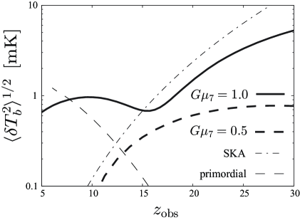
Figure 3: The rms fluctuations of the differential brightness temperature due to string wakes. The thick solid and dashed lines represent the rms fluctuations for $G\mu_{7}=1.0$ and $0.5$, respectively, where $G\mu_{7}$ denotes the normalized $G\mu$ in units of $10^{-7}$. The SKA noise is plotted as the thin dashed line.

5 Conclusion

In this paper, we have evaluated the redshifted 21 cm fluctuations due to minihalos in cosmic wakes. Cosmic strings produce string wakes, and wakes fragment to minihalos in the early universe. Although minihalos due to strings can dominate nonlinear structures at high redshifts, the virial temperature is below 200 K in our models. Accordingly, they cannot contribute to star and galaxy formation with atomic cooling and even hydrogen molecular cooling. However, we have shown that they can create 21 cm line signals, because the density and temperature of neutral hydrogen in minihalos are high enough to make the spin temperature of minihalos decouple from the CMB temperature and differ from the background spin temperature. The signals are emission lines against CMB at low redshifts, while they are observed as absorption lines.

Since minihalos due to cosmic strings are clustered in string wakes, they can strongly enhance the angular fluctuations of redshifted 21 cm signals integrated over the line of sight. We have evaluated the root-mean-square fluctuations due to minihalos clustered in string wakes with a toy model of string networks. The amplitude of the fluctuations due to wake minihalos becomes large as the redshift increases. Therefore, these fluctuations can dominate those due to minihalos induced by primordial density fluctuations at high redshifts, even if the cosmic string tension is smaller than the current upper limit, $G\mu\sim 10^{-7}$. In order to estimate the feasibility of the constraint on $G\mu$ by SKA, we have compared the 21 cm fluctuations from minihalos due to string wakes with the SKA noise. Although the SKA noise increases rapidly at high redshifts, we have found that the fluctuations from such minihalos with $G\mu\sim 7.5\times 10^{-8}$ at $10<z<15$ is potentially detectable by SKA.

Here we have considered only one frequency band to evaluate the detection limit on $G\mu$ by SKA. However, SKA will observe a large range of frequency and many frequency bands will be available. A multi-frequency analysis of 21 cm signals can increase the signal to noise (SN) ratio. We have performed the SN ratio analysis for SKA multi-frequency observation whose redshift range is $7<z<15$. We have found that, for the multi-frequency observation, the SN ratio with $G\mu=4.0\times 10^{-8}$ becomes larger than one.

The rms fluctuations are enhanced by the number density of minihalos in string wakes. In this paper, we have calculated the rms fluctuations, making simple assumptions about the fragmentation of string wakes. The number density of minihalos strongly depends on the process of fragmentation from wakes. For a detailed study of the fragmentations, numerical simulations are essential. We will address these issues in a future paper.

The amplitude of the rms fluctuations due to strings also depends on the details of the string network. However, our calculation is based on a simple toy model of a scaling solution. Although we have not considered the case of a network, string loops are also produced in the evolution of string networks. The loops can induce early structure formation and contribute to the 21 cm fluctuations. To take into account loop contributions, our future calculations will be applied with a self-consistent string network model including the loop distributions.

References

- [1] T. W. B. Kibble, Topology of cosmic domains and strings, Journal of Physics A Mathematical General 9 (Aug., 1976) 1387–1398.
- [2] A. Vilenkin and E. P. S. Shellard, Cosmic strings and other topological defects. 1994.
- [3] M. B. Hindmarsh and T. W. B. Kibble, Cosmic strings, Reports on Progress in Physics 58 (May, 1995) 477–562
- [4] I. B. Zeldovich, Cosmological fluctuations produced near a singularity, MNRAS 192 (Sept., 1980) 663–667.
- [5] A. Vilenkin, Cosmological density fluctuations produced by vacuum strings, Physical Review Letters 46 (Apr., 1981) 1169–1172.
- [6] J. Silk and A. Vilenkin, Cosmic strings and galaxy formation, Physical Review Letters 53 (Oct., 1984) 1700–1703.
- [7] A. Albrecht, R. A. Battye, and J. Robinson, The Case against Scaling Defect Models of Cosmic Structure Formation, Physical Review Letters 79 (Dec., 1997) 4736–4739.
- [8] L. Pogosian, S.-H. H. Tye, I. Wasserman, and M. Wyman, Observational constraints on cosmic string production during brane inflation, Phys. Rev. D 68 (July, 2003) 023506.
- [9] M. Wyman, L. Pogosian, and I. Wasserman, Bounds on cosmic strings from WMAP and SDSS, Phys. Rev. D 72 (July, 2005) 023513.
- [10] Planck Collaboration, P. A. R. Ade, N. Aghanim, C. Armitage-Caplan, M. Arnaud, M. Ashdown, F. Atrio-Barandela, J. Aumont, C. Baccigalupi, A. J. Banday, and et al., Planck 2013 results. XXV. Searches for cosmic strings and other topological defects, ArXiv e-prints (Mar., 2013) [arXiv:1303.5085].
- [11] L. Pogosian and A. Vilenkin, Early reionization by cosmic strings reexamined, Phys. Rev. D 70 (Sept., 2004) 063523.
- [12] K. D. Olum and A. Vilenkin, Reionization from cosmic string loops, Phys. Rev. D 74 (Sept., 2006) 063516.
- [13] B. Shlaer, A. Vilenkin, and A. Loeb, Early structure formation from cosmic string loops, J. Cosmology Astropart. Phys. 5 (May, 2012) 26, [arXiv:1202.1346].
- [14] H. Tashiro, E. Sabancilar, and T. Vachaspati, Constraints on superconducting cosmic strings from early reionization, Phys. Rev. D 85 (June, 2012) 123535, [arXiv:1204.3643].
- [15] F. Duplessis and R. Brandenberger, Note on structure formation from cosmic string wakes, J. Cosmology Astropart. Phys. 4 (Apr., 2013) 45, [arXiv:1302.3467].
- [16] S. R. Furlanetto, S. P. Oh, and F. H. Briggs, Cosmology at low frequencies: The 21 cm transition and the high-redshift Universe, Phys. Rep. 433 (Oct., 2006) 181–301.
- [17] J. R. Pritchard and A. Loeb, 21 cm cosmology in the 21st century, Reports on Progress in Physics 75 (Aug., 2012) 086901, [arXiv:1109.6012].
- [18] M. Tegmark and M. Zaldarriaga, Omniscopes: Large area telescope arrays with only NlogN computational cost, Phys. Rev. D 82 (Nov., 2010) 103501, [arXiv:0909.0001].
- [19] R. H. Brandenberger, R. J. Danos, O. F. Hernández, and G. P. Holder, The 21 cm signature of cosmic string wakes, J. Cosmology Astropart. Phys. 12 (Dec., 2010) 28, [arXiv:1006.2514].
- [20] O. F. Hernández, Y. Wang, R. Brandenberger, and J. Fong, Angular 21 cm power spectrum of a scaling distribution of cosmic string wakes, J. Cosmology Astropart. Phys. 8 (Aug., 2011) 14, [arXiv:1104.3337].
- [21] O. F. Hernández and R. H. Brandenberger, The 21 cm signature of shock heated and diffuse cosmic string wakes, J. Cosmology Astropart. Phys. 7 (July, 2012) 32, [arXiv:1203.2307].
- [22] E. McDonough and R. H. Brandenberger, Searching for signatures of cosmic string wakes in 21cm redshift surveys using Minkowski Functionals, J. Cosmology Astropart. Phys. 2 (Feb., 2013) 45, [arXiv:1109.2627].
- [23] M. Pagano and R. Brandenberger, The 21 cm signature of a cosmic string loop, J. Cosmology Astropart. Phys. 5 (May, 2012) 14, [arXiv:1201.5695].
- [24] H. Tashiro, 21 cm angular spectrum of cosmic string loops, Phys. Rev. D 87 (June, 2013) 123535, [arXiv:1305.4779].
- [25] I. T. Iliev, P. R. Shapiro, A. Ferrara, and H. Martel, On the Direct Detectability of the Cosmic Dark Ages: 21 Centimeter Emission from Minihalos, ApJ 572 (June, 2002) L123–L126.
- [26] S. R. Furlanetto and A. Loeb, The 21 Centimeter Forest: Radio Absorption Spectra as Probes of Minihalos before Reionization, ApJ 579 (Nov., 2002) 1–9.
- [27] P. R. Shapiro, K. Ahn, M. A. Alvarez, I. T. Iliev, H. Martel, and D. Ryu, The 21 cm Background from the Cosmic Dark Ages: Minihalos and the Intergalactic Medium before Reionization, ApJ 646 (Aug., 2006) 681–690.
- [28] A. Meiksin, The micro-structure of the intergalactic medium - I. The 21 cm signature from dynamical minihaloes, MNRAS 417 (Oct., 2011) 1480–1509, [arXiv:1102.1362].
- [29] S. Chongchitnan and J. Silk, The 21-cm radiation from minihaloes as a probe of small primordial non-Gaussianity, MNRAS 426 (Oct., 2012) L21–L25, [arXiv:1205.6799].
- [30] A. Vilenkin, Gravitational field of vacuum domain walls and strings, Phys. Rev. D 23 (Feb., 1981) 852–857.
- [31] L. Perivolaropoulos, R. H. Brandenberger, and A. Stebbins, Dissipationless clustering of neutrinos in cosmic-string-induced wakes, Phys. Rev. D 41 (Mar., 1990) 1764–1774.
- [32] S. M. Miyama, S. Narita, and C. Hayashi, Fragmentation of Isothermal Sheet-Like Clouds. I —Solutions of Linear and Second-Order Perturbation Equations—, Progress of Theoretical Physics 78 (Nov., 1987) 1051–1064.
- [33] A. C. Quillen and J. Comparetta, Jeans Instability of Palomar 5’s Tidal Tail, ArXiv e-prints (Feb., 2010) [arXiv:1002.4870].
- [34] R. Barkana and A. Loeb, In the beginning: the first sources of light and the reionization of the universe, Phys. Rep. 349 (July, 2001) 125–238.
- [35] G. B. Field, Excitation of the Hydrogen 21-CM Line, Proceedings of the IRE 46 (Jan., 1958) 240–250.
- [36] M. Kuhlen, P. Madau, and R. Montgomery, The Spin Temperature and 21 cm Brightness of the Intergalactic Medium in the Pre-Reionization era, ApJ 637 (Jan., 2006) L1–L4.
- [37] R. K. Sheth and G. Tormen, Large-scale bias and the peak background split, MNRAS 308 (Sept., 1999) 119–126.
- [38] P. R. Shapiro, I. T. Iliev, and A. C. Raga, A model for the post-collapse equilibrium of cosmological structure: truncated isothermal spheres from top-hat density perturbations, MNRAS 307 (July, 1999) 203–224.
- [39] I. T. Iliev and P. R. Shapiro, The post-collapse equilibrium structure of cosmological haloes in a low-density universe, MNRAS 325 (Aug., 2001) 468–482.