A new approach to detailed structural decomposition
from the SPLASH and PHAT surveys:
Kicked-up disk stars in the Andromeda Galaxy?

Abstract

We characterize the bulge, disk, and halo subcomponents in the Andromeda galaxy (M31) over the radial range $4~{}{\rm kpc}<R_{\rm proj}<225$ kpc. The cospatial nature of these subcomponents renders them difficult to disentangle using surface brightness (SB) information alone, especially interior to $\sim 20$ kpc. Our new decomposition technique combines information from the luminosity function (LF) of over $1.5$ million bright $(20<m_{\rm 814W}<22)$ stars from the Panchromatic Hubble Andromeda Treasury (PHAT) survey, radial velocities of over $5000$ red giant branch stars in the same magnitude range from the Spectroscopic and Photometric Landscape of Andromeda’s Stellar Halo (SPLASH) survey, and integrated $I$-band SB profiles from various sources. We use an affine-invariant Markov chain Monte Carlo algorithm to fit an appropriate toy model to these three data sets. The bulge, disk, and halo SB profiles are modeled as a Sérsic, exponential, and cored power-law, respectively, and the LFs are modeled as broken power-laws. We present probability distributions for each of 32 parameters describing the SB profiles and LFs of the three subcomponents. We find that the number of stars with a disk-like LF is $5.2\pm 2.1\%$ larger than the the number with disk-like (dynamically cold) kinematics, suggesting that some stars born in the disk have been dynamically heated to the point that they are kinematically indistinguishable from halo members. This is the first kinematical evidence for a “kicked-up disk” halo population in M31. The fraction of kicked-up disk stars is consistent with that found in simulations. We also find evidence for a radially varying disk LF, consistent with a negative metallicity gradient in the stellar disk.

1. INTRODUCTION

Spiral galaxies like the Milky Way (MW) and Andromeda (M31) are composed of several structural subcomponents, each with its own formation history. Tracing the evolution of such a galaxy, then, depends on characterization of the individual subcomponents. This decomposition is especially difficult in the inner regions, where the cospatial bulge, disk, and halo complicate characterization of any single subcomponent.

The most commonly used way to characterize the stellar component of a large spiral galaxy is via surface brightness (SB) decomposition. SB profiles of disks tend to fall off exponentially, whereas bulges follow more general Sérsic profiles [Sérsic, 1968]. Widely used SB decomposition codes such as GIM2D [Simard, 2002] and GALFIT [Peng et al., 2002] fit a sum of a Sérsic spheroid and an exponential disk to the SB distribution of a galaxy to estimate the relative contributions of the components. Unfortunately, such fitting is plagued by degeneracies that arise because the different subcomponents are cospatial and because the procedure generally relies on ad hoc fitting formulae that do not necessarily separate the galaxy into dynamically distinct subcomponents [e.g., Abadi et al., 2003].

In this paper, we present a new technique for decomposing the stellar component of M31 into distinct bulge, disk, and halo subcomponents. This technique can be applied to any galaxy close enough to measure radial velocities and a luminosity function of stars down to about 1.5 magnitudes fainter than the tip of the red giant branch (TRGB). In addition to fitting a toy model (exponential disk, powerlaw halo, and Sérsic bulge) to the SB distribution, we attempt to break the aforementioned degeneracies by including an additional constraint: the fraction of stars that belong to the disk (“disk fractions”), as measured from stellar kinematics of individual red giant branch (RGB) stars. We perform the decomposition using Bayesian techniques so that we can identify covariances between model parameters, quantifying lingering degeneracies.

Two large-scale, ongoing resolved stellar population surveys of M31 make it an ideal galaxy in which to develop and test our decomposition technique. The Spectroscopic and Panchromatic Landscape of Andromeda’s Stellar Halo (SPLASH) survey has used the Keck/DEIMOS multiobject spectrograph to measure radial velocities of over 15,000 stars in M31 [Guhathakurta et al., 2005, 2006], including over 10,000 in the crowded inner 20 kpc [Dorman et al., 2012, Gilbert et al., 2012, Howley et al., 2013]. Meanwhile, the Panchromatic Hubble Andromeda Treasury (PHAT) survey, a five-year Hubble Space Telescope/Multi-Cycle Treasury (HST/MCT) program, has so far imaged over $10^{8}$ stars in six filters in the UV, optical, and near-IR in the same quadrant of the disk most densely sampled by SPLASH [Dalcanton et al., 2012].

The decomposition technique presented here builds directly on the work of Courteau et al. [2011] and Dorman et al. [2012]. The former performed SB-only decompositions of M31 using two different techniques: Markov chain Monte Carlo (MCMC) sampling and a nonlinear least-squares (NLLS) fitting method. In each case, the authors fit a sum of Sérsic bulge, exponential disk, and powerlaw halo to I-band SB profiles of the galaxy. The profiles were a composite of major- and minor- axis cuts of an $I$-band image of the central $\sim 20$ kpc of M31 [Choi et al., 2002] plus minor-axis profiles measured from RGB star counts [Pritchet & van den Bergh, 1994, Irwin et al., 2005, Gilbert et al., 2009]. They found that the best-fit bulge, disk, and halo structural parameters depended significantly on the decomposition method, data points used (major vs. minor axis), and even on the binning of the data. Despite the uncertain results, their model was still relatively restrictive, not allowing for a flattened halo or for variations from the canonical values in the ellipticities or position angles of the bulge and disk.

In Dorman et al. [2012], we performed a kinematical decomposition of M31’s dynamically cold disk (without distinguishing between thin and thick components) and dynamically hot spheroid (without distinguishing between bulge or halo components) using radial velocity measurements of $\sim 6000$ bright ($20<I<22$) RGB stars in the inner parts of the galaxy ($5<R_{\rm proj}<20$ kpc; the region dominated by the disk in optical and UV images). In each of $24$ small spatial subregions, we measured the fraction of stars that belonged to the hot component. This fraction is nonzero ($>10\%$) everywhere in the survey region. The origin of this dynamically hot population is unclear a priori: is it an outward extension of the central bulge or the innermost reaches of the extended halo? On one hand, the bulge appears too small in SB decompositions to contribute stars past a few kpc [Courteau et al., 2011]; on the other hand, CMD analyses of fields between $11$ and $45$ kpc on the minor axis reveal populations with young/intermediate ages and intermediate metallicities [Brown et al., 2003, Richardson et al., 2008] — quite unlike the old, metal-poor halo field stars in the MW [e.g., Carollo et al., 2007, Kalirai, 2012].

In this paper, we use kinematically derived disk fractions measured as in Dorman et al. [2012] as constraints in a SB decomposition of M31’s $I$-band SB profile. Simultaneously fitting to the total SB profile of the galaxy and the fraction contributed by the disk may help to reduce degeneracies in the best fit parameters — and possibly understand the structural association and origin of the dynamically hot population identified in Dorman et al. [2012]. With more constraints, we can relax some of the assumptions made in Courteau et al. [2011], fitting for the ellipticities and position angle of the bulge, disk, and halo.

A primary challenge in our work is that our disk fraction measurements come from star count data, whereas we model the contributions to the integrated surface brightness. Thus, we must convert a disk fraction in star counts to a disk fraction in SB units. In general, this conversion factor is such that the kinematical survey undersamples the disk: the SPLASH target selection function happens to peak at magnitudes where the spheroid and disk both contribute stars, and to fall off at brighter magnitudes where only the disk contributes light. In addition, while it is easily recoverable, the selection function is somewhat arbitrary, varying across the galaxy. In order to quantify how fairly it samples the three subcomponents, we model and fit for the disk, bulge, and halo luminosity functions (LFs).

The model presented here incorporates stellar population, kinematics, and SB data for the first time. Including complexities like the boxy bulge [Beaton et al., 2007] or separate thin, thick, and extended disks [Collins et al., 2011, Ibata et al., 2005] are beyond the scope of the paper, which nonetheless our analysis represents a significant improvement over using only SB profile fits to characterize a galaxy’s physical components.

This paper is organized as follows. First, in § 2, we outline the analysis procedures that will be described in detail in § 3-4. In § 3 we summarize the kinematical, integrated-light, and resolved stellar photometric data sets used as constraints. In § 4 we present the mathematical formalism used to find the probability distribution functions (PDFs) of each of the model parameters. In § 5 we discuss the probability distributions of our parameters, comparing them to previous measurements of M31’s structural parameters. In § 6, we show that the dynamically hot population in our kinematical sample is more closely associated with the extended halo than the central bulge, and propose that some fraction of that population originated in the disk. Finally, we summarize in § 7.

2. Overview of Analysis Procedure

Simultaneously fitting even a simple toy model to the observed SB map, disk fractions, and LF is relatively complicated. We must process three different data sets, develop a multiparameter model, combine the model and data into a likelihood function, and sample that likelihood to obtain a probability distribution function (PDF) for each parameter. Each of these steps will be described in detail in § 3-4, but first we will present a brief road map to those sections.

The flow chart in Figure 1 illustrates the path from data processing to model parameter PDFs. We start with three sets of observational constraints: SB profiles, the kinematically-derived disk fraction probability distribution in each of the spatial subregions, and the $F814W$ ($I$) LF in each subregion. The processing of these three data sets is described in § 3.1-3.3.

As the left-hand side of Figure 1 shows, each data set has an accompanying toy model. We model the SB as the sum of three profiles: a Sérsic bulge, an exponential disk, and a cored power-law halo (§ 4.1.1). Similarly, we model the luminosity function as a sum of three broken powerlaws, one each for the disk, bulge, and halo, in the magnitude range $m_{\rm F814W}=[20,22]$ (§ 4.1.3). The model for the disk fraction comes from a combination of the previous two: the disk fraction in flux units at a given location is the ratio of the disk to total SB at that location; however, we must convert this integrated-light disk fraction to star counts using the disk LF (§ 4.1.2).

Given a certain vector $w$ in parameter space, we compute the probability $P_{\rm SB}(w)$ that the SB model represents the observed SB map; similarly, we define and compute $P_{\rm f}(w)$ and $P_{\rm LF}(w)$ as the probabilities that the model matches the kinematical and LF data sets, respectively. The total probability of that vector $w$ is then $P(w)=P_{\rm SB}P_{\rm f}P_{\rm LF}$. § 4.2 gives the equation for $P$.

We then sample this probability distribution $P$ using the Markov chain Monte Carlo (MCMC) sampler emcee [Foreman-Mackey et al., 2013], as described in § 4.3. The sampler yields a PDF of each model parameter. In § 5, we discuss the median values and confidence intervals of the PDFs in the context of previous measurements.

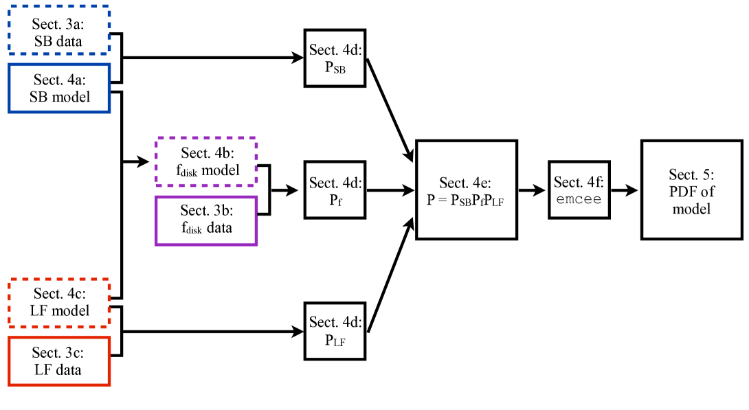
Figure 1.— Flow chart illustrating the analysis procedure. Each box is labeled with the section of the text in which that step is described. See text of § 2 for description.

3. Observational Constraints

The integrated-light, resolved stellar photometric, and spectroscopic data sets used in this work are described in more detail in Courteau et al. [2011], Gilbert et al. [2012], Dalcanton et al. [2012], and Dorman et al. [2012]. In this section we briefly recap the salient information.

3.1. Surface Brightness

The SB map is derived from two classes of data: major- and minor-axis wedge cuts from a mosaic image, and RGB star counts. All of the profiles are in the $I$ band to minimize the effects of inhomogeneities such as dust lanes or the UV-bright star-forming rings. The SB data used in this work are identical to those used in Courteau et al. [2011], with the addition of new halo fields out to a galactocentric projected radius of $R=225$ kpc first presented in Gilbert et al. [2012].

3.1.1 Integrated Light Profiles

We use the major- and minor-axis SB profiles of M31 that Courteau et al. [2011] constructed from an $I$-band CCD mosaic image of M31 taken with the Kitt Peak National Observatory Burrell Schmidt telescope and presented in Choi et al. [2002]. Rather than relying on azimuthally averaged isophotal fitting, which smears together components with very different ellipticities such as bulge and disk, they cut wedges from the major and minor axes of the galaxy. They measured the median SB in each of 186 bins on the major axis and 152 on the minor axis. The sizes of the bins increased with galactocentric radius. Bright stars were removed via an iterative sigma-clipping process. The quoted error bar in each bin is the RMS deviation about the median value of the pixels in that bin. The locations of these bins on the sky are marked as teal circles in Figure 2 and in Figure 3, the latter zooming in on the the portion of the galaxy dominated by the bright disk and bulge.

Because the CCD pixel size is $2^{\prime\prime}$ and the telescope was not well focused during some of the observations, some of the images that went into the final mosaic image are out of focus at the $2^{\prime\prime}-5^{\prime\prime}$ level. (See § 2 of Choi et al. [2002].) To avoid the effects of finite spatial resolution, we exclude from our analysis the two bins within projected radius $R=10^{\prime\prime}~{}(40~{}\rm pc)$ of the center of M31.

3.1.2 Star Counts

In the outer regions of the galaxy, where crowding is less severe, the SB profile can be measured, up to a normalization factor, from RGB star counts. Like Courteau et al. [2011], we have combined the extended star counts of the M31 stellar halo by Pritchet & van den Bergh [1994], Irwin et al. [2005], Gilbert et al. [2009], and Gilbert et al. [2012]. These profiles cover the range $20~{}{\rm kpc}<R<225$ kpc.

The Pritchet & van den Bergh [1994] data set — which combines digital star counts to measure the SB in three fields along the minor axis of the galaxy — is identical to that used in Courteau et al. [2011]. These fields are marked in yellow squares in Figures 2 and 3.

The Irwin et al. [2005] data set is also identical to that used in Courteau et al. [2011]. Irwin et al. [2005] combined the data from Pritchet & van den Bergh [1994] with faint RGB star counts to trace the minor-axis stellar distribution out to a projected radius of $55$ kpc. They used star counts from the Isaac Newton Telescope, exposing typically $800-1000$ s per field in the Gunn $i$ band. These fields are shown as blue triangles in Figures 2 and 3.

The final SB data set, presented in Gilbert et al. [2009] and Gilbert et al. [2012], is based on RGB star counts from a Keck/DEIMOS spectroscopic survey of 38 fields between $9-225$ kpc in projected radius [rather than just the 12 fields used by [Courteau et al., 2011]]. Members of M31’s smooth halo were identified and distinguished from foreground MW dwarf star contaminants and substructure in the M31 halo using a combination of photometric and spectroscopic diagnostics [Guhathakurta et al., 2006, Gilbert et al., 2006]. To estimate M31’s stellar surface density as a function of radius, the observed ratio of M31 red giants to MW dwarf stars was multiplied by the surface density of MW dwarf stars predicted by the Besançon Galactic star-count model [e.g., Robin et al., 2003, 2004]. The surface density was converted to SB units by scaling to match the minor axis profile from Choi et al. [2002]. These fields are shown as magenta stars in Figures 2 and 3.

In summary, we have 637 SB measurements $\mu_{\rm obs}$ from 4 data sets. Though the SB data are given in magnitudes, we perform the SB fits using flux units; the conversion is given through the usual formula:

$$\displaystyle\Sigma_{\rm obs}(R,\Delta PA)=10^{-(\mu_{\rm obs}+zp)/2.5}$$ (1)

where $\Sigma_{\rm obs}$ is in flux units, $\mu_{\rm obs}$ is in magnitudes, and $zp$ is the zeropoint. To ensure consistency between datasets, we anchor the zeropoints of the Pritchet & van den Bergh [1994], Gilbert et al. [2012], and Irwin et al. [2005] datasets to that of the Choi et al. [2002] image by first fitting to the composite SB map only (i.e., not including constraints on the disk fraction), leaving the zeropoint as a free parameter with a flat prior between $\pm 2$ magnitude of the Choi et al. [2002] value. For each dataset, the median (best fit) zeropoint of the resulting posterior distribution is adopted for the rest of the analysis.

The composite, zeropoint-adjusted major- and minor-axis SB profiles are shown in the two panels of Figure 4.

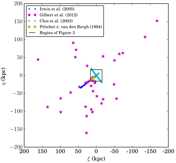
Figure 2.— Locations of 637 fields from 4 datasets used for SB measurements. The Choi et al. [2002] measurements (teal circles) come from a wedge cut of an I-band image from KPNO; the rest of the SB measurements, including Irwin et al. [2005] (blue triangles), Gilbert et al. [2012] (violet stars), and Pritchet & van den Bergh [1994] (yellow squares) are derived from RGB star counts. The inner black box has a side length of 32 kpc, approximately the size of the GALEX image of M31. A zoom-in of this region is shown in Figure 3.

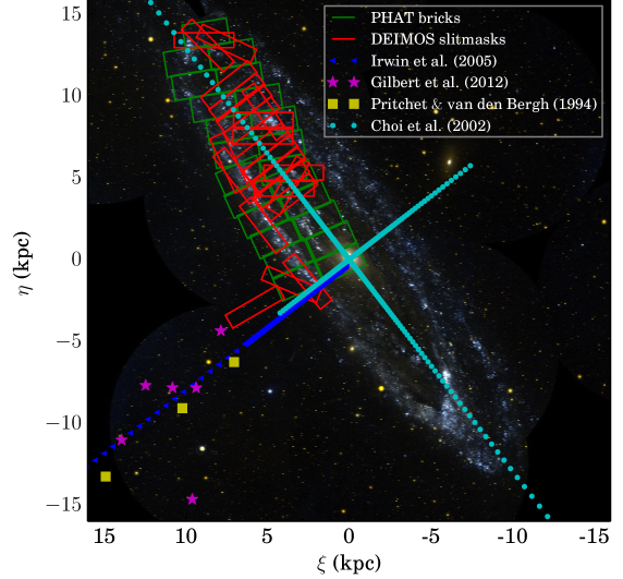
Figure 3.— Zoom-in on the map of SB fields from Figure 2 that fall in the inner regions of M31, overlaid on a GALEX image. Points are color-coded as in Figure 2. The Irwin et al. [2005] points (blue triangles) are drawn slightly offset from the minor axis for clarity; they actually overlap the Choi et al. [2002] minor axis points (teal circles). For comparison, bricks in the HST PHAT survey (from which we measure the bright end of the luminosity function) are shown in green and Keck/DEIMOS slitmasks from the SPLASH survey (from which we measure radial velocities of RGB stars) are outlined in red. The kinematical and LF analyses presented in this paper are carried out in the regions where the green bricks and red slitmasks overlap.

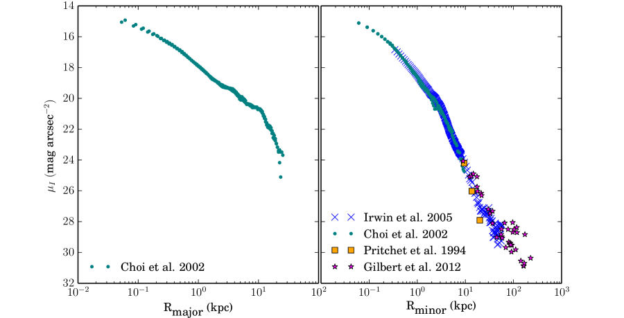
Figure 4.— Major- (left) and minor- (right) axis projections of the SB profiles, assuming a major axis position angle of $37.7^{\circ}$. Samples from opposite sides of the galactic center are collapsed onto a single set of axes. Gilbert et al. [2012] points (violet stars) do not lie on either axis, so for display purposes we project them to the minor axis assuming a circularly symmetric halo. Photometric uncertainties are typically smaller than the point size.

3.2. Velocity distribution

The constraints on the fraction of stars dynamically associated with the disk are obtained via a kinematical decomposition of the stellar velocity distribution into dynamically cold (disk) and hot (spheroid, or combined bulge and halo) components, described in detail in Dorman et al. [2012].

3.2.1 Kinematical data

We obtain spectra of 5257 stars in the inner 20 kpc of M31 using the DEIMOS multi-object spectrograph on the Keck II telescope as part of the SPLASH survey [Guhathakurta et al., 2005, 2006, Gilbert et al., 2009, Dorman et al., 2012, Howley et al., 2013]. The positions of the 29 DEIMOS slitmasks are shown as red rectangles overlaid on a GALEX image of M31 in Figure 3. The targets on 19 of these masks contain targets selected from an $i^{\prime}$-band CFHT/MegaCam image, while the targets on 5 masks were selected exclusively from the PHAT catalog and the targets on the remaining 5 were selected using a combination of PHAT and CFHT data. In each case, the targets are selected based on a complex set of factors: apparent degree of isolation in the source catalog, magnitude bright enough to yield a high-S/N spectrum but not so bright as to be a likely foreground MW dwarf, and position on the sky so as to optimize the use of the slitmask. Hence, the luminosity function of DEIMOS-observed stars is different in each slitmask, but in general is nonzero between $20<i^{\prime}<22$ and peaks somewhere around $i^{\prime}\sim 21$.

Each spectrum is collapsed in the spatial direction and cross-correlated against a suite of template rest-frame spectra to measure its radial velocity. The velocity measurement is then quality-checked by eye, and only robust velocities (those based on at least two strong spectral features) are included in the analysis.

We perform a number of cuts on this preliminary kinematical dataset. First, we retain only the 3247 (63% of) targets that are also present in the existing PHAT catalog. (The other targets lie in regions on the sky not sampled by the PHAT survey at the time of writing.) Second, we cut out the 25% of the remaining objects that are located in regions with $A_{v}>1.0$ mag. The low extinction regions were identified by modeling the NIR CMD as a sum of a foreground unreddened RGB and a background RGB, reddened by a log-normal distribution of dust reddening, in 10 arcsecond bins. This modeling produced a map of the median $A_{V}$ across the disk, independent of the fraction of reddened stars along a given line of sight. Details can be found in Dalcanton et al. (2013, in prep), and an overview of the technique can be found in Dalcanton et al. [2012]. All of the 2443 remaining stars are redder than $m_{\rm F475W}-m_{\rm F814W}=1.5$, so are likely to be RGB stars rather than bright main sequence (MS) objects. In the following text, we describe how we use these 2443 stars to measure disk fractions in each of 14 spatial subregions.

3.2.2 Review of Disk Fraction Measurements

In Dorman et al. [2012], the SPLASH and PHAT survey region was divided into four spatial “regions”: three straddling the NE major axis and one along the SE minor axis. The boundaries of the regions (lines of constant $R_{\rm proj}$ or position angle P.A.) were chosen such that each region contained enough SPLASH targets to constrain the velocity distribution of the subdominant spheroid component. Each region was then subdivided along lines of constant P.A. into multiple “subregions,” each large enough to contain $>100$ stars but small enough that the rotation velocity of the disk component does not vary substantially. We measured the mean velocity $v$, velocity dispersion $\sigma_{v}$, and fraction $f$ of the disk and spheroid components in each of the resulting 24 subregions by fitting a sum of two Gaussians (representing a dynamically cold disk and dynamically warmer spheroid) to the velocity distribution in each subregion.

Because in the current paper we use only the subset of spectroscopic targets also identified in the PHAT survey, we must combine some subregions from Dorman et al. [2012] to have sufficient number statistics to reliably separate the disk and spheroid. The 14 subregions we use are shown in the right-hand panel of Figure 5. The subregions are named using the same formalism as in Dorman et al. [2012]. The survey area is still divided into four regions: SE (along the SE minor axis), and NE1, NE2, and NE3 (along the NE major axis, in order of increasing projected radius). The subregions within each region are identified with subscripts that increase with distance from the major axis: $\rm NE1_{1},NE1_{2},\ldots,NE1_{5};~{}NE2_{1},\ldots,NE2_{4}$, and $\rm NE3_{1},NE3_{2},NE3_{3}.$ In the SE region, the inner south, and inner north subregions are named $\rm SE_{2}$ and $\rm SE_{3},$ respectively. (Subregion $SE_{1}$ is not used because it does not overlap with the PHAT survey region.)

We fit a sum of two Gaussians (representing a dynamically cold disk and dynamically warmer spheroid) to the velocity distribution in each subregion with the MCMC sampler emcee [Foreman-Mackey et al., 2013, see the Appendix for more information]. We allow the disk velocity distribution to change from subregion to subregion, but require that the mean velocity and dispersion of the spheroid remain constant between subregions within a region. The decomposition makes almost no assumptions about the nature of the disk, except that its velocity distribution is symmetric and locally colder than that of the spheroid.

The latter is perfectly reasonable; however, one could imagine that asymmetric drift in a stellar disk could skew the distribution of circular velocities towards lower speeds and upweighting the spheroid in the decomposition. We found that asymmetric drift does not in fact have a significant effect on the kinematically derived disk fractions. We tested the effects of asymmetric drift using the velocity distribution presented in Schönrich & Binney [2012] to measure disk fractions in the major axis subregions, where the effect of asymmetric drift should be most significant. In near-major-axis subregions ($NE1_{1-3}$, $NE2_{1-2}$, $NE3_{1-3}$), the disk fractions computed by assuming symmetric and asymmetric velocity distributions are consistent to within $1\sigma$. In subregions that are closer to the minor axis, it is difficult to fit the asymmetric function to the velocity distribution because the line-of-sight velocity measurements do not well constrain the rotation velocity. However, for the same reason, we expect the effects of asymmetric drift on the measured disk fraction to be decrease towards the minor axis. The line-of-sight velocity of a star on the minor axis is independent of the circular velocity of that star, and so a slight change in the circular velocity distribution should not affect the line-of-sight distribution. Therefore, we can safely ignore the effect of asymmetric drift and use a Gaussian disk velocity distribution without affecting the disk fraction measurements.

Figure 6 illustrates the velocity decomposition in each subregion within a representative region, NE2, which is centered along the northeast major axis at a projected radius of about 10 kpc. Note that in each subregion within the NE2 region, some nonzero fraction of stars belong to the dynamically hot component. Nearly half of these spheroid stars are counterrotating relative to the disk (that is, they have radial velocities less than $v_{\rm M31}=-300$ km/s), and thus must be spheroid stars regardless of the detailed shape of the disk velocity distribution. In § 6, we will show that these stars are more closely associated with the extended halo than the central bulge, and that some of them likely originated in the disk.

The cold fraction in each subregion $s$ is the ratio of the areas of the cold Gaussian and the total velocity distribution. At the end of the 10,000-step MCMC chain, the disk fractions measured from the 32 walkers over the final 2000 steps of the chain are compiled and binned by $0.5\%$ into a normalized PDF $p_{s}(f_{\rm d})$.

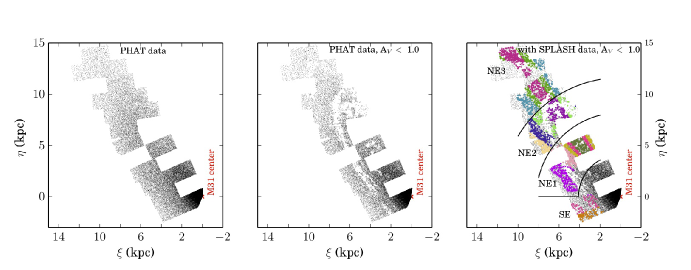
Figure 5.— Map of target locations in the PHAT and SPLASH surveys. Left: Stars in the magnitude range $m_{F814W}=[20,22]$ in PHAT. (Only a random 4% of the objects are shown.) Middle: Same as left panel, but without stars in dusty ($A_{v}>1.0$) pixels. The star-forming $10$ kpc ring is effectively excluded. Right: Same as middle panel, with stars from the SPLASH survey in non-extincted regions overplotted as colored dots. Black lines separate the 4 large “regions,” while colors demarcate the 14 smaller “subregions.” The $F814W$ luminosity functions and kinematically-derived disk fractions are measured in each subregion, where the kinematical and PHAT surveys overlap. Note that the central few kpc are not used in the fits to the kinematics and LF, because this region is too crowded for resolved stellar spectroscopy with DEIMOS.

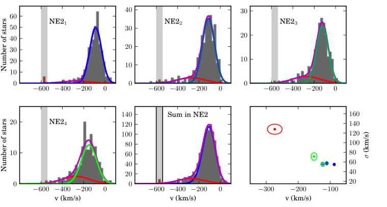
Figure 6.— First four panels: fits to the velocity distribution of RGB stars from the SPLASH survey in each of four subregions in the NE2 (middle northeast major axis) region, plotted over velocity histograms of stars in each subregion. Each velocity distribution is fit by a sum of two Gaussians corresponding to a dynamically hot spheroid (red) and dynamically cold disk (blue to green). The sum of the two curves is shown in violet. Velocity ranges excluded from the fits due to possible contamination by tidal debris from the Giant Southern Stream (GSS) are shown in two equivalent ways: by the gray shaded regions and by the stars shaded red on the histogram. Bottom middle panel: Sum of hot components in the NE2 region (red curve) and sum of cold components (blue curve) overplotted on a histogram of all radial velocities in NE2. Bottom right panel: Ellipses represent the mean and uncertainty of each of the parameter pairs $(v,\sigma_{v})$. The four blue and green ellipses represent the kinematical parameters of the disk components in the four subregions. The red ellipse respresents the spheroid component, which has the same $(v,\sigma_{v})$ in every subregion within this region.

Because it will be more useful to have an analytic form for $p_{s}(f_{\rm d})$, we fit a skew-normal function $\phi_{s}$ to $p_{s}(f_{\rm d})$ in each subregion $s$ using a Levenberg-Marquardt minimization. The form of $\phi_{s}$ is

$$\displaystyle\phi_{s}(f)=A_{s}e^{-(z_{s}/\sqrt{2})^{2}}\bigg{(}1+{\rm erf}\bigg{(}\frac{\tau_{s}z_{s}}{\sqrt{2}}\bigg{)}\bigg{)}$$ (2)

where

$$\displaystyle z_{s}=(f_{s}-\mu_{s})/\sigma_{s}.$$ (3)

The best-fit skew-normal parameters $\mu_{s},\sigma_{s},\tau_{s}$, along with the medians and standard deviations of the $p_{s}$ distributions, are given in Table 1. Figure 7 shows an example fit to $p_{s}(f_{\rm d})$ in representative subregion $\rm NE2_{4}$. The PDFs are very well approximated by a skew-normal function: the $\chi^{2}~{}p$-statistic is 1.000 in every subregion. The uncertainties in the disk fraction measurements in each subregion are parameterized by the width of the skew-normal function; the entire function (not just an error bar) will be used as a prior on the disk fraction in the decomposition presented. Note that because the subregions are our smallest resolution elements in our kinematical analysis, we cannot map the variation in kinematically-derived disk fraction within a subregion. However, in subregions where the true disk fraction varies significantly, the PDF is broad — in other words, systematic uncertainties in the measured disk fractions derived from finite spatial binning are incorporated into the error bars.

Table 1Skew-Normal Parameters of
Disk Fraction Probability Distribution $p_{s}(f_{\rm d})$

Subregion	$\mu$	$\sigma$	$\tau$	A	Median	Std. dev.
${\rm{NE1_{1}}}$	0.75	0.11	-1.64	1.83	0.68	0.08
${\rm{NE1_{2}}}$	0.82	0.11	-1.73	1.86	0.75	0.08
${\rm{NE1_{3}}}$	0.56	0.11	-0.78	1.88	0.51	0.09
${\rm{NE1_{4}}}$	0.83	0.22	-1.65	0.95	0.70	0.15
${\rm{NE1_{5}}}$	0.77	0.10	-1.11	1.97	0.72	0.08
${\rm{NE2_{1}}}$	0.96	0.04	-2.43	4.61	0.93	0.03
${\rm{NE2_{2}}}$	0.86	0.08	-2.04	2.4	0.81	0.06
${\rm{NE2_{3}}}$	0.87	0.08	-2.00	2.57	0.82	0.05
${\rm{NE2_{4}}}$	0.84	0.15	-2.53	1.38	0.75	0.10
${\rm{NE3_{1}}}$	0.83	-0.04	1.47	5.12	0.81	0.03
${\rm{NE3_{2}}}$	0.86	0.05	-1.35	4.04	0.84	0.04
${\rm{NE3_{3}}}$	0.84	0.06	-1.34	3.50	0.81	0.04
${\rm{SE_{2}}}$	0.30	0.25	-0.07	4.53	0.33	0.21
${\rm{SE_{3}}}$	-2.68	3.16	-1.26	19.30	0.37	0.29

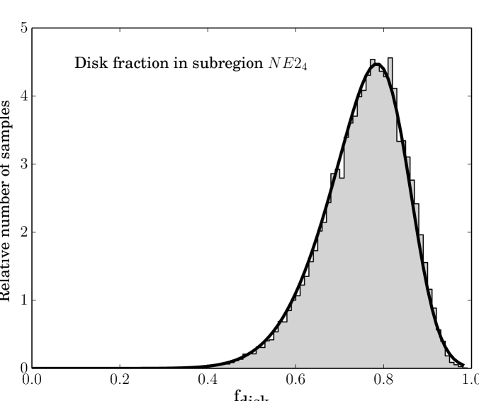
Figure 7.— Probability distribution of the kinematically derived disk fraction in the off-major-axis subregion $\rm{NE2}_{4}$. The gray filled histogram is constructed from 50,000 samples from the end of the MCMC chain used to fit the sum of two Gaussians (disk and spheroid) to the observed velocity distribution in this subregion. The black curve represents the skew-normal function $\phi$ that best fits the histogram. $\phi$ is later used as the prior on the disk fraction; that is, a model that predicts a disk fraction near the peak (e.g., $f_{\rm d}\sim 0.8$) will be more favorable than one that predicts a disk fraction far from the peak (e.g., $f_{\rm disk}\sim 0.3$).

3.3. Luminosity Function

The bright end of M31’s LF is the crucial link between the kinematical and SB data. The kinematics measure the fraction of stars, as sampled by the SPLASH survey, that belong to the disk in each small subregion, while a SB decomposition yields the fraction of integrated light contributed by the disk. To convert between these units, we must know how fairly the SPLASH survey samples the bulge, disk, and halo LFs. We therefore fit three model LFs to the observed PHAT LF in each subregion. This section describes the observed LF; the model LFs are discussed in § 4.1.3.

We measure the PHAT LF in the magnitude range sampled by SPLASH ($20<m_{\rm F814W}<22$). While the PHAT survey is crowding-limited and thus incomplete at faint magnitudes, within our radial range,$6<R<20$ kpc in deprojected radius, it is $100\%$ complete down to $m_{\rm F814W}=22$ for colors $m_{\rm F475W}-m_{\rm F814W}<4.5$. (We have tried a decomposition excluding the few percent of stars redder than this cutoff, but the qualitative results are not affected.) We clean the sample in the same way as for the SPLASH data set, using only stars redder than $m_{F475W}-m_{F814W}=1.5$ and in pixels with $A_{v}<1.0$ mag. We bin these stars by $0.1$ mag in the range $20<m_{F814W}<22$. Figure 5 shows the PHAT stars in this magnitude range before (left) and after (right) excluding stars in extincted regions.

In each subregion $s$, we measure two normalized luminosity functions in the magnitude range sampled by the SPLASH spectroscopic survey $(I=[20,22])$. $\mathcal{L}_{\rm PHAT,s}$ contains stars from the PHAT catalog that fall into subregion $s$. $\mathcal{L}_{\rm SPLASH,s}$ contains stars found in both the SPLASH and PHAT surveys in subregion $s$. Each has units of number/$\textrm{arcsec}^{2}$/mag. The uncertainty on each observed LF is simply the Poisson counting uncertainty on each bin $\sqrt{N}$, where $N$ is the number of stars in the subregion that fall into that magnitude bin.

We display the PHAT and SPLASH luminosity functions from two representative subregions in Figure 8. The shape of the PHAT LF is similar in all subregions: the slope is shallow at the faint end, gradually steepens brightward of $m_{\rm F814W}\sim 21$, and finally flattens again brightward of $m_{\rm F814W}\sim 20.5$. These changes in slope can be explained by the position of the TRGB in M31 and the presence of intermediate-age stars brighter than the TRGB. The magnitude of the TRGB at the distance of M31 is $m_{I}=20.35$ near $[M/H]=-1$, changing by only about $0.1$ dex between $-2.5<[M/H]<-0.57$ [Salaris & Cassisi, 1997]. However, the metallicity distribution of M31’s disk and bulge extend to supersolar values [Sarajedini & Jablonka, 2005, Brown et al., 2006]. At such high metallicities, line blanketing in the red can push the TRGB even fainter than $m_{I}=21$. The wide shoulder seen in the PHAT LF between the TRGB and $m_{\rm F814W}\sim 21$ is a signature of a broad metallicity distribution with a broad range of TRGB magnitudes. The shallow slope brightward of the metal-poor TRGB at $m_{\rm F814W}=20.35$ suggests a high fraction of young or intermediate-age populations with bright AGB stars, as described by Méndez et al. [2002].

The SPLASH luminosity function varies from subregion to subregion, but usually peaks in the range $20.5<m_{\rm F814W}<21.5$ due to the design of the spectroscopic survey. (Targets in this magnitude range were bright enough to yield high-quality spectra, but faint enough to likely be M31 members rather than foreground MW dwarfs, so they were given highest priority in the target selection process.) Because there are so many fewer stars in the SPLASH sample than in PHAT, for display purposes we have scaled the SPLASH LF by a factor of 100, and scaled the Poisson errors accordingly.

We can measure the spectroscopic selection function $S_{s}(M)$ in each subregion $s$:

$$\displaystyle S_{s}(M)=\mathcal{L}_{\rm SPLASH,s}/\mathcal{L}_{\rm PHAT,s}$$ (4)

$S_{s}(M)$ is a purely empirical measure of the complicated target selection criteria of the spectroscopic survey. Examples of $S_{s}(M)$ in two representative subregions are shown in the bottom panels of Figure 8. The variation in the selection function with subregion and with magnitude means that the SPLASH survey may over- or under-sample the spheroid relative to the disk. We correct for this effect, as described late in the following section.

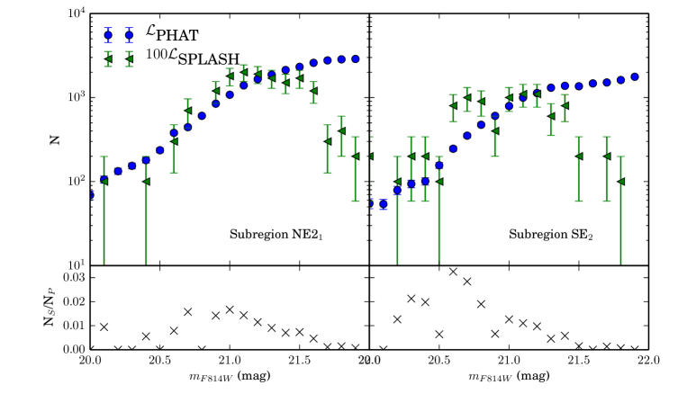
Figure 8.— Top panels: PHAT (blue) and SPLASH (green) luminosity functions (LFs) in two subregions: NE2₁, which lies on the major axis, and SE₂, which lies on the minor axis. The SPLASH LF has been scaled by a factor of 100. Error bars represent Poisson uncertainties. Note that the slope of the PHAT LF changes twice: at $m_{\rm F814W}\sim 20.4$ mag (the TRGB of a population with $[M/H]\lesssim-0.6$) and around $21$ mag (the TRGB of a more metal-rich population). Bottom panels: The empirical selection function $N_{\rm SPLASH}/N_{\rm PHAT}$ is shown for each subregion. The selection function varies from subregion to subregion.

4. Analysis

Our goal is to find the most probable combination of structural and LF parameters for a Sérsic bulge, exponential disk, and power-law halo given the three sets of constraints described above: surface brightness, PHAT LF in each of 14 subregions, and kinematically-derived disk fraction in each subregion. As shown in Figure 1, we build a toy model to represent the SB, disk fraction and LF across the galaxy. In § 4.1 we describe our model: a 2D surface brightness profile and LF for each structural subcomponent. In § 4.2 we show the likelihood function to be sampled. Finally, in § 4.3, we describe the Markov chain Monte Carlo sampler emcee [Foreman-Mackey et al., 2013] that we use to sample the parameter space.

4.1. Model

The model parameters are listed in the first column of Table 2. All parameters have flat priors within the range specified in the fourth column of the table. The only fixed parameter is the bright-end slope (log $N$/mag = $500$/mag) of the halo LF, chosen for reasons described in § 4.1.3.

4.1.1 Surface Brightness Profiles

As discussed in the introduction, we choose simple, standard SB profiles for three components: the bulge, disk, and halo. Each profile is given in terms of position on the sky $(R,PA)$, where $R$ is the projected radius and and $PA$ is the position angle measured east of north. Hence, we can fit to an entire SB map, rather than only to data points that happen to fall on the major or minor axis. We assume that the three model components have the same major axis position angle $pa$.

Bulge

For the bulge, we assume a generalized Sérsic profile with Sérsic index $n_{b}$, half-light radius $R_{b}$ and intensity $I_{b}$ at $R_{b}$:

$$\displaystyle\Sigma_{b}(R_{\rm eff,b})=I_{b}\exp\left\{-A_{n_{b}}\left[\bigg{(}\frac{R_{\rm eff,b}}{R_{b}}\bigg{)}^{1/n_{b}}-1\right]\right\}$$ (5)

$$\displaystyle R_{\rm eff,b}(R,\Delta PA,\epsilon_{b})=R\sqrt{\cos^{2}\Delta\rm PA+\bigg{(}\frac{\sin\Delta\rm PA}{1-\epsilon_{b}}\bigg{)}^{2}}$$ (6)

$$\displaystyle\Delta PA=PA-pa$$ (7)

where $A_{n_{b}}=1.9992n_{b}-0.3271$ [Capaccioli, 1989]. The formula is given in terms of the effective major axis (deprojected) coordinate $R_{\rm eff,b}$, which is a function of the major axis position angle $pa$ and bulge ellipticity $\epsilon_{b}$. With $n_{b}=1$ or $n_{b}=4$, the profile reduces to the exponential or de Vaucouleurs profile, respectively.

Disk

We assume an exponential SB profile for the disk:

$$\displaystyle\Sigma_{d}(R_{\rm eff,d})=I_{d}\exp{(-R_{\rm eff,d}/R_{d})},$$ (8)

where $I_{d}$ is the disk surface brightness at the galactic center and $R_{d}$ is the scale length in the plane of the disk. The formula is given in terms of deprojected radius $R_{\rm eff,d}$, computed as before in terms of ($R,\Delta\rm PA$) and disk ellipticity $\epsilon_{d}$.

Halo

Finally, we assume a 2D cored power-law halo SB profile. Though it is also possible to model a halo as a Sérsic function, we adopt a power-law because Courteau et al. [2011] demonstrate that such a model is a more reasonable description of the M31 halo. The halo surface brightness is then given as

$$\displaystyle\Sigma_{h}(R_{\rm eff,h})=\frac{I_{h}}{(1+(R_{\rm eff,h}/R_{h})^{2})^{\alpha/2}}$$ (9)

where $I_{h}$ is the halo surface brightness at the galactic center, $R_{h}$ is the radius of the core, and the effective major axis coordinate $R_{\rm eff,h}$ is defined as before in terms of coordinates $(R,\Delta PA)$ and halo ellipticity $\epsilon_{h}$.

We define

$$\displaystyle\Sigma_{T}(R,\Delta PA)=\Sigma_{b}+\Sigma_{d}+\Sigma_{h}$$ (10)

to be the total surface brightness of the model at coordinates $(R,\Delta PA)$.

For each profile, we fit for the central intensity in units of $\rm mag~{}arcsec^{-2}$ rather than $\rm counts~{}arcsec^{-2}$. So our model parameters describing central magnitudes are $\mu_{b},~{}\mu_{d},~{}\mu_{h}$ rather than $I_{b},~{}I_{d},~{}I_{h}$. The three central magnitude parameters $\mu_{k}$ are defined as follows:

$$\displaystyle\mu_{b}=-2.5\log_{10}I_{b}+25.6$$ (11)

$$\mu_{d}=-2.5\log_{10}I_{d}+25.6$$ (12)

$$\mu_{h}=-2.5\log_{10}I_{h}+25.6$$ (13)

Here the zeropoint $25.6$ is chosen to match that of the Choi et al. [2002] SB data.

Because the fractional photometric uncertainties $e_{m}$ on the SB measurements are typically very small, we introduce an uncertainty parameter $\epsilon_{\rm SB}$ into the model to allow for additional photometric uncertainty as well as departures from the assumed functional form of the SB profile. $\epsilon_{\rm SB}$ is allowed to have a unique value for each SB dataset $j$, but may not vary between points $i$ within a given data set. The total fractional uncertainty of a given SB measurement $\Sigma_{ij}$ is then the quadrature sum of the Poisson uncertainty and the error parameter:

$$\displaystyle\epsilon_{ij}=\Sigma_{ij}\sqrt{e^{2}_{m,ij}+\epsilon_{{\rm SB},j}^{2}}$$ (14)

4.1.2 Disk Fractions

We have measured the disk fraction distribution $\phi_{s}(f_{d})$ in each subregion $s$, and we want to know what disk fraction our SB model predicts. The fraction of integrated I-band light contributed by the disk is of course $\Sigma_{d}/\Sigma_{T}$. However, to compare this to a kinematically-derived disk fraction, we must convert it to a fraction of stars, as sampled by the somewhat arbitrary SPLASH survey, contributed by the disk. This conversion requires knowledge of the intrinsic disk luminosity function $\mathcal{L}_{d}$, the total luminosity function $\mathcal{L}_{T}$, and the subregion-specific SPLASH selection function $S_{s}(m_{\rm F814W})$. The model disk fraction in SPLASH star count units in subregion $s$ is

$$\displaystyle f_{\rm d,s}=\frac{\int S_{s}n_{d,s}\mathcal{L}_{d}dm_{\rm F814W}}{\int S_{s}n_{t,s}\mathcal{L}_{T,s}dm_{\rm F814W}}$$ (15)

where the integration only needs to be performed over the magnitude range $m_{\rm F814W}=[20,22]$, where the SPLASH selection function is nonzero.

Later in this paper (section 5.4), we will use a conversion factor $C_{s}$ to convert between disk fraction units. $C_{s}$ is defined as the ratio between $f_{\rm d,s}$ (the disk fraction as measured in SPLASH star counts, as defined in Equation 15) and the disk fraction as measured in SB units:

$$\displaystyle C_{s}\equiv\frac{f_{\rm d,s}}{\Sigma_{d,s}/\Sigma_{T,s}}.$$ (16)

$C_{s}$ is constant within a subregion $s$, but varies from subregion to subregion.

As with the SB data, we introduce a kinematical uncertainty parameter $e_{k}$ (expressed as a fraction of the empirical skew-normal width $\sigma_{s}$) to account for non-ideal $f_{\rm d}$ calculation due to, e.g., any non-Gaussianity in the disk line-of-sight velocity distribution. We add this parameter in quadrature to $\sigma_{s}$ and re-normalize the widenened skew-normal PDF.

4.1.3 Luminosity Functions

Equation 15 shows that computing the predicted disk fraction $f_{\rm d}$ (in star count units) requires knowledge of the disk luminosity function $\mathcal{L}_{d}$ in the magnitude range $m_{\rm F814W}=[20,22]$. Therefore, we model the bright end of the disk, bulge, and halo luminosity functions. This magnitude range includes the tip of the red giant branch (TRGB), which lies near $m_{\rm F814W}=20.5$ at the distance of M31 for stars with $[M/H]\lesssim-0.5$ and fainter for more metal-rich populations (see discussion in § 3.3).

Because RGB stars dominate the stellar population faintward of the TRGB, while younger objects such as AGB stars fill in the brightward portion of the LF, there is reason to expect that the number density of stars should fall at different rates faintward and brightward of the TRGB. Hence, we parameterize the LF of each component $k$ = (disk, bulge, halo) as a broken powerlaw in log(number density) vs. magnitude space:

$$\displaystyle\log\mathcal{L}_{k}(m_{\rm F814W})=c_{0k}+\begin{cases}p_{k}m&{~{}m<l_{k}}\\ q_{k}m+l_{k}(p_{k}-q_{k})&{~{}m\geq l_{k}}\\ \end{cases}\$$ (17)

where $c_{0k}$ is chosen such that $\mathcal{L}_{k}$ is normalized to unity over this magnitude range.

Since it is reasonable to expect that the stellar disk may have an age or metallicity gradient, we allow each of the disk LF parameters to depend linearly on radius on the plane of the disk $R_{\rm eff,d}$ in the radial range of interest $5~{}{\rm kpc}<R_{\rm eff,d}<20$ kpc:

$$\displaystyle p_{d}=p_{d0}+\delta p_{d}\ln(R_{\rm eff,d})$$ (18)

$$q_{d}=q_{d0}+\delta q_{d}\ln(R_{\rm eff,d})$$ (19)

$$l_{d}=l_{d0}+\delta l_{d}\ln(R_{\rm eff,d})$$ (20)

However, for simplicity, we require that the power-law slopes $p,q$ and the break magnitude $l$ for the bulge and the halo be constant with radius. This assumption does not affect our results, since the portion of the galaxy covered by the LF and kinematical surveys is almost entirely disk-dominated according to SB-only decompositions [Courteau et al., 2011] as well as our decomposition. Even if the halo does contribute a significant number of stars in the SPLASH survey region, its range of metallicities is confined to the metal-poor regime [Kalirai et al., 2006], where the magnitude of the TRGB is insensitive to metallicity. Near the end of Section 6.1, we discuss this point further.

We require for each component that $p,q$ be nonnegative within the radial range $5~{}{\rm kpc}<R_{\rm eff,d}<20$ kpc, and that $l$ lie within the magnitude range of interest, $m_{F814W}=[20,22]$. We also require that the bright-end slope of the halo LF to be extremely steep ($p_{h}=500$, because an old component should not have stars brighter than the TRGB) and that the break magnitude of each component be fainter than the brightest expected TRGB components ($l_{k}<20.3$).

The total normalized LF ${\mathcal{L}_{T,s}}$ in subregion $s$ is then the weighted sum of those of the disk, bulge, and halo, where the weights correspond to the number density of stars in each subcomponent in the magnitude range of interest. To compute the weights, we assume that in each component, the ratio of the number density $n_{k}$ of stars in the range $I=[20,22]$ to the surface brightness $\Sigma_{k}$ of that component is a constant $y_{k}$. Hence, we introduce four new model parameters $y_{b},~{}y_{h},~{}y_{d0},$ and $\delta y_{d}$, defined by the following relationships:

$$\displaystyle y_{b}\equiv\frac{n_{b,s}}{\Sigma_{b,s}}$$ (21)

$$y_{h}\equiv\frac{n_{h,s}}{\Sigma_{h,s}}$$ (22)

$$y_{d}(R_{\rm eff,d})\equiv\frac{n_{d,s}}{\Sigma_{d,s}}$$ (23)

$$y_{d}(R_{\rm eff,d})=y_{d0}+R_{\rm eff,d}\delta y_{d}$$ (24)

where $\Sigma_{k,s}$ is the average surface brightness of subcomponent $k$ integrated over the area of subregion $s$. The ratio $y_{k}$ is a constant independent of subregion $s$ for the bulge and for the halo, and depends linearly on $R_{\rm eff,d}$ for the disk. Then the total number density of stars in subregion $s$ is

$$\displaystyle n_{t,s}=(y_{d0}+R_{\rm eff,d}\delta y_{d})\Sigma_{d,s}+y_{b}\Sigma_{b,s}+y_{h}\Sigma_{h,s}$$ (25)

and the normalized model LF is

$$\displaystyle{\mathcal{L}}_{T,s}(m)=\frac{n_{d,s}{\mathcal{L}}_{d}+n_{b,s}{\mathcal{L}}_{b}+n_{h,s}{\mathcal{L}}_{h}}{n_{t,s}}$$ (26)

As with the SB and kinematical data, we introduce an uncertainty parameter $\epsilon_{\mathcal{L}}$ to account for differences between the assumed broken power law and the actual shape of the LF. $\epsilon_{\mathcal{L}}$ is a fractional uncertainty whose value is constant across all magnitude bins and all subregions. The total fractional uncertainty on a given LF bin $m$ and subregion $s$ is the quadrature sum of the Poisson fractional uncertainty and $\epsilon_{\mathcal{L}}$. Then the total uncertainty on that LF bin is

$$\displaystyle\epsilon_{LF,m,s}=\mathcal{L}_{\rm PHAT,m,s}\sqrt{\frac{1}{N_{m,s}}+\epsilon_{\mathcal{L}}^{2}}.$$ (27)

4.2. Model-Data Comparison: Likelihood Function

The probability that a point in parameter space is a good representation of the data is given by the product of three goodness-of-fit statistics describing the agreement between the model and the three data sets:

$$\displaystyle P=P_{\rm SB}P_{\rm LF}P_{\rm f_{d}}$$ (28)

We work instead with the log-likelihood:

$$\displaystyle\ln P=\ln P_{\rm SB}+\ln P_{\rm LF}+\ln P_{\rm f_{d}}$$ (29)

The SB factor is summed over each data point $i$ in each data set $j$:

$$\displaystyle\ln P_{\rm SB}=-\sum_{i,j=1}^{N,n_{i}}\left[\frac{(\Sigma_{T,ij}-\Sigma_{{\rm obs},ij})^{2}}{2\pi\epsilon_{ij}^{2}}\right]$$ (30)

Meanwhile, the LF and disk fraction factors are summed over each of the 14 subregions. The goodness-of-fit to the disk fraction is the height of the skew-normal function $\phi_{s}(f_{\rm d})$ that describes the probability distribution of the kinematically measured disk fraction in subregion $s$, evaluated at the model disk fraction $C_{s}\frac{\Sigma_{d,s}}{\Sigma_{T,s}}$:

$$\displaystyle\ln P_{\rm f}=\sum_{s=1}^{14}\ln\phi_{s}\bigg{(}f_{\rm d}=C_{s}\frac{\Sigma_{d,s}}{\Sigma_{T,s}}\bigg{)}$$ (31)

The LF component of the likelihood is determined by summing the difference between the observed and model total luminosity functions over every magnitude bin $m$ in every subregion $s$:

$$\displaystyle\ln P_{\rm\mathcal{L}}=-\sum_{s,m=1}^{14,20}\frac{(n_{p,s}\mathcal{L}_{{\rm PHAT},s,m}-n_{T,s}\mathcal{L}_{T,s,m})^{2}}{\epsilon_{LF,s,m}^{2}}.$$ (32)

4.3. MCMC Sampler

To estimate the probability distribution function of each model parameter, we draw samples from the log-likelihood function (Equation 29) using the the Markov chain Monte Carlo sampler emcee [Foreman-Mackey et al., 2013]. More details on emcee can be found in the Appendix. This section will only summarize the details unique to this paper.

In emcee, and more generally MCMC, an ensemble of “walkers” — or points in parameter space — moves through parameter space. During each step, each walker is given the option to move a specified distance along the line in parameter space connecting it to a random other walker. Moves corresponding to increases in the value of the likelihood function are always accepted; moves corresponding to decreases in likelihood are sometimes accepted. After many steps (the “burn-in” phase), the distribution of walkers samples the likelihood function: the density of walkers is highest in high-probability regions of parameter space. In this paper, we allow 256 walkers to burn in for 10,000 steps, and analyze the probability distributions using their positions in their last 100 steps. These probability distributions are shown in Figures 19 and 20 in the Appendix.

5. Results

5.1. Confidence Intervals & Correlations

We measure the mean value and $1\sigma$ confidence interval for each parameter from its posterior probability distribution. We report these statistics in Table 2. In general, the parameters describing the SB profiles are very well constrained, to better than $1\%$, while the LF parameters are constrained to $10\%$ at best.

Some of the parameters appear in Table 2 to be completely unconstrained, but in fact are simply strongly correlated with other parameters. For a given such pair, the allowed region in 2D space can be quite small. To quantify covariances between parameters, we calculate the Spearman correlation coefficient $r$ between every pair of parameters. Those pairs with $r^{2}>0.6$ are labeled “strongly correlated”, while those with $0.25<r^{2}<0.6$ are labeled “significantly correlated.” Figure 9 shows the 2D probability distributions of 24 of the 28 strongly or significantly correlated pair of parameters.

All six of the strongly correlated pairs, and all but four of the significantly correlated pairs, consist of two parameters describing the same subcomponent. For example, the bulge effective radius $R_{b}$ is significantly correlated with the bulge Sérsic index $n_{b}$, but not with the disk or halo scale radii. Similarly, the disk LF bright-end slope $p_{d0}$ depends on the disk LF break magnitude $l_{d0}$, but not on the slopes or break magnitudes of the bulge or halo LFs. Additionally, with a few exceptions, the SB parameters tend to be correlated only with other SB parameters, while the LF parameters tend to be correlated only with other LF parameters.

5.2. Quality of Profile Fits

Because the degeneracy between parameters is generally confined to within a subcomponent, the subcomponent SB and LF profiles are well constrained and are not degenerate with one another. The middle panel of Figure 10 shows a minor axis projection of the SB decomposition into bulge, disk, and halo subcomponents. One set of profiles (bulge, disk, and halo) is displayed for each of 256 samples drawn from the last step of the walker ensemble. The set of 256 violet lines, then, samples the entire range of bulge profiles allowed by the data; similarly, the set of 256 red lines represents the entire allowed range of disk profiles. Note that the profiles are relatively well constrained: for example, while the bulge scale radius $R_{b}$ and Sérsic index $n_{b}$ each vary significantly, they covary in such a way that the bulge is always small, contributing less SB than the halo at only $R\sim 4$ kpc on the minor axis.

The LF decomposition in each of three representative subregions is shown in Figure 11. The disk (red dotted line) dominates in every subregion, so that it is nearly indistinguishable from the total model LF (orange shaded region) or observed PHAT LF (blue line with error bars). For clarity, in this plot we only display the bulge, disk, and halo LFs corresponding to the median values of the parameters. However, in Figure 12 we display the three LFs normalized in the magnitude range $20<m_{\rm F814W}<22$, with one line drawn for each of 256 samples in the walker ensemble. Since the shape of the disk LF is allowed to change with radius, we display two representative disk LFs: one at the radius of an inner subregion (red lines) and one at the radius of an outer subregion (gold lines). The disk LF is tightly constrained at any given radius despite the significant degeneracy between the slopes and central values of the individual LF parameters. The bulge (violet) and halo (green) LFs are also relatively well constrained, especially considering that neither component dominates in any subregion sampled by our portion of the PHAT survey.

The model fits the SB and LF data sets quite well. The bottom panel of Figure 10 displays the difference between the observed and best-fit SB profiles expressed in units of SB uncertainty (a combination of Poisson measurement errors and error parameter). The fit to the SB is very good: the magnitude error is generally less than 10% of the SB uncertainty, corresponding to a median reduced $\chi^{2}$ of $0.82$. The fit to the LF is also acceptable, with a median $\chi^{2}$ of $0.81$. However, the fit to the kinematics is less satisfactory (median reduced $\chi^{2}=1.88$). Figure 13 shows that the model overestimates the disk fraction in almost every subregion, and by more than $1\sigma$ in four subregions. Though the measured disk fractions do constrain the model, their limited number and relatively large uncertainties mean that they have less effect on the final decomposition than the LF and SB data, which strongly prefer a small Sérsic component and dominant exponential component. The poor fit to some of the kinematical measurements is then a sign of tension between our (very simple) model and the data. In § 6.1, we show that allowing for a dynamically hot ($\sigma_{v}\sim 150~{}\rm km~{}s^{-1}$) component with disklike population and spatial profile (a “kicked-up disk”) can reduce this tension.

The decompositions presented in Figures 10 and 12 will be discussed in more detail later in this section (§ 5.3) and in the Discussion (§ 6).

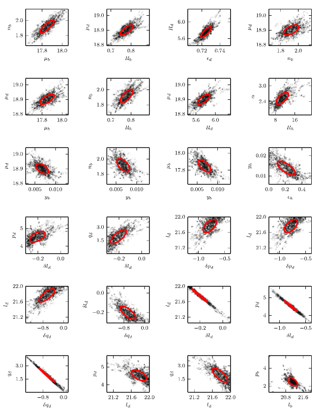
Figure 9.— 2D posterior distributions of 24 of the strongly (Spearman $r^{2}>0.6$) or significantly ($0.6\geq r^{2}>0.25$) correlated pairs of parameters. (Only 28 of the 512 pairs of parameters fall into one of these categories.) Red dashed contours are $1\sigma$ error ellipses. In general, a parameter is correlated only with other parameters describing the same subcomponent (bulge, disk or halo). LF parameters tend to be correlated only with other LF parameters, and SB parameters only with other SB parameters.

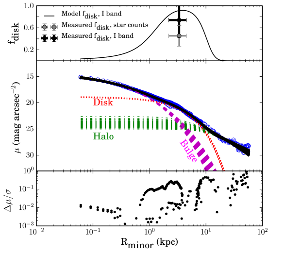
Figure 10.— Minor axis SB decomposition. Middle: Fit of the model SB profile (black lines) to the observed SB profile (blue circles) as a function of projected radius. The model is also shown decomposed into the disk (red dotted), halo (green dot-dashed), and bulge (magenta dashed) components. One line is displayed for each of 256 samples drawn from the posterior distribution of walkers, so that the width of each region encloses the entire uncertainty (not the $1\sigma$ uncertainty) associated with that profile. The disk, inner bulge, and outer halo profiles are well constrained, whereas the inner halo and outer bulge profiles are less well constrained. Top: Model disk fraction in SB units (black line) slightly overpredicts kinematically measured disk fraction in the minor axis subregion ($SE_{2}$) converted to SB units (black cross). The conversion factor from disk fraction in star counts (gray cross) to disk fraction in SB units (black cross) is about $1.2$ in this subregion: the kinematical survey oversamples the spheroid population. Bottom: Average residual between model and measured SB as a function of projected radius, relative to the measurement uncertainties on the SB. The lower and upper tracks between 0.3 and 2.5 kpc correspond to the Choi and Irwin data sets, respectively.

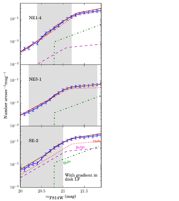
Figure 11.— Comparison between observed PHAT (blue) and model (brown) total normalized LFs after a fit to the SB with kinematical constraints, assuming radial gradients in the disk LF shape parameters, in three representative subregions. The shaded portion shows where the SPLASH selection function is at least 30% of its maximum value. The model is shown decomposed into disk (red), bulge (magenta), and halo (green) components. Each LF is weighted by the number density of stars in the magnitude range $F814W=[20,22]$ in that subcomponent in the subregion of interest. The width of the brown region is given by the variation in the model LF. Error bars on the PHAT LF include contributions from both the $\sqrt{N}$ Poisson uncertainty in each $0.1$ mag bin and the LF uncertainty parameter.

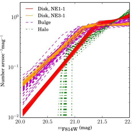
Figure 12.— Normalized median bulge (magenta), disk (red, orange), and halo (green) LFs. For each component, one line is displayed for each of 256 samples drawn from the posterior distribution of walkers, so that the width of each region encloses the entire uncertainty (not the $1\sigma$ uncertainty) associated with that profile. The disk LF depends on radius in the plane of the disk $R_{\rm d}$; the disk LFs in the subregions with smallest and largest $R_{\rm d}$ are displayed in red and orange, respectively, to illustrate the range in disk LF over the PHAT survey region.

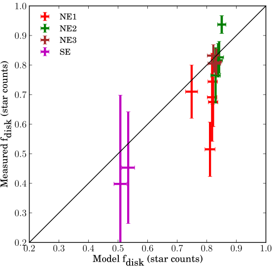
Figure 13.— Comparison between the measured cold and model disk fractions, in units of SPLASH star counts, in the final decomposition. Error bars reflect estimated $1\sigma$ uncertainties from the appropriate distributions at the end of the MCMC chain. Points are color-coded by spatial region. Measured cold fractions are systematically lower than model disk fractions, suggesting that there may be a dynamically hot (“kicked-up”) disk component for which our model has not accounted.

5.3. Comparison to previous measurements

The median values of our parameters are presented in Table 2. Here, we compare some of the structural parameters to previous measurements.

The disk scale length we measure, $5.76\pm 0.1$ kpc, is consistent with the range of accepted values. Worthey et al. [2005] measure an $R_{d}=5.8\pm 0.2~{}\rm kpc$ from elliptical isophotal fits to the Choi I-band image alone. Seigar [2008] measure $R_{d}=5.91\pm 0.27$ kpc from an IRAC $3.6~{}\mu m$ profile. Ibata et al. [2005] measured a scale length of $5.1\pm 0.1~{}\rm kpc$ by fitting an exponential profile to RGB star counts in the range $R=20-40$ kpc on the major axis — though if the spheroid actually contributes some additional light in the inner part of that radial range, the disk profile could appear to fall off faster than it actually does, and so the authors would underestimate the disk scale length.

Our $R_{d}$ is nearly $0.8$ kpc ($16\%$) larger than that measured in the same band with an SB-only decompostion (Model U in Courteau et al. [2011]). This offset is likely to arise because we fit for the position angle of the disk, whereas Courteau et al. [2011] simply assume a position angle of $37.7^{\circ}$. The scale length of a disk is largest when measured along its true major axis (that is, when the position angle is correct).

Our median disk ellipticity, $0.725\pm 0.005$, corresponds to an inclination of $74.0^{\circ}\pm 0.3^{\circ}$ in the infinitely thin limit. The HI disk at similar radii has a similar inclination [Chemin et al., 2009, Corbelli et al., 2010]. Overall, the optical disk appears about three degrees closer to edge-on, though M31’s badly warped outer disk [Chemin et al., 2009, Corbelli et al., 2010] implies a strong dependence of inclination on radius. Additionally, the older populations that we sample are more likely to have been heated and thickened via satellite interactions at some point in their lifetimes, making the RGB disk appear more face-on than the younger stellar disk.

Our disk position angle ($44.4^{\circ}\pm 0.5^{\circ}$) is $6-8$ degrees greater than that of the HI disk in the $R\sim 5-20$ kpc range [Chemin et al., 2009, Corbelli et al., 2010], but is similar to that seen in the azimuthal number density of all RGB stars in the PHAT dataset [Dalcanton et al., 2012].

Our bulge is nearly identical to that found in the SB-only decomposition of Courteau et al. [2011]. The Sérsic index ($1.92\pm 0.08$) is intermediate between exponential and de Vaucouleurs, characteristic of a disky “pseudobulge.” [Kormendy & Kennicutt, 2004].

Athanassoula & Beaton [2006] and Beaton et al. [2007] have found that NIR photometry and HI/H$\alpha$ kinematics are reproduced by N-body models with at least two bulge components: a small classical bulge, a larger boxy pseudobulge, and a bar that may extend beyond the pseudobulge. We do not distinguish between these subcomponents; instead, our $n=1.9$ Sérsic bulge includes all of them. As described later (end of § 6.1), we also try to model a two-component bulge by fitting the sum of an exponential, a power-law, and two Sérsic profiles to the composite data set, but the highest-likelihood models are exclusively the single-Sérsic ones.

The core radius of the halo, $R_{h}=10.6^{+2.5}_{-2.0}$ kpc, is signficantly larger than the value of $3$ kpc measured from a fit to the number density profile of resolved blue horizontal branch (BHB) stars [Williams et al., 2012]. This quantity is in general difficult to measure, since it relies on tracing the halo in the inner regions of the galaxy, where the faint halo is strongly subdominant to the disk and bulge. Our technique is one of the few that does not involve fixing other structural parameters or using only a single halo tracer such as BHB stars or RGB stars. As shown in Figure 9, $R_{h}$ is degenerate with the power-law halo slope $\alpha$, but is very unlikely to be shorter than $8$ kpc and is not degenerate with any other parameters.

The power-law slope of the halo profile external to the core is $-2.5\pm 0.2$, consistent with measurements from SB-only decompositions [Courteau et al., 2011], resolved RGB star counts [Guhathakurta et al., 2005, Gilbert et al., 2012] and BHB star counts [Williams et al., 2012]. A projected surface density power-law slope of $-2.5$ corresponds to a deprojected density that scales approximately as $r^{-3.5}$, in good agreement with cosmologically motivated simulations in which stellar halos are built up via accretion [e.g., Bullock & Johnston, 2005, Cooper et al., 2010] and accretion plus in situ star formation [e.g., Font et al., 2011]. The outer slope of a Navarro, Frenk & White [1996] cold dark matter halo also scales as $r^{-3.5}$, suggesting that stars may trace the dark matter profile — but not significantly affect its shape — at large radii.

5.4. Conversion between integrated-light and star-count disk fractions

The conversion factor between disk fraction as measured in integrated light and disk fraction as measured in SPLASH star counts ($C_{s}$ in Equation 16) is $0.84-0.86$ in the subregions near the major axis and $0.62-0.65$ near the minor axis. $C<1$ implies that the spectroscopic survey is biased towards spheroid stars — not a surprise, since the spectroscopic target selection strategy prioritizes less crowded objects and spheroid stars are less likely to be located in clusters or clumpy structures. In the discussion that follows, as in the analysis, this correction has been applied to the model so that both the model and measured disk fractions represent the fraction of stars, as sampled by the SPLASH survey, that contribute to the disk.

6. Discussion

We discuss three classes of new results. First, we argue that a fraction of the stars in M31’s dynamically hot inner spheroid may have originated in the disk. Second, we discuss the transition between the bulge and halo. Third, we discuss the evidence for a radial gradient in the LF of M31’s stellar disk.

6.1. Kicked-up disk

Despite the significant dynamically hot population in the kinematical sample, both the SB and LF data are best fit by a model with a bulge too small to contribute light in the SPLASH survey region. Figures 10 and Figure 11 illustrate the fits. Figure 10 shows that the SB profile on the minor axis between projected radii of $1-10$ kpc — the radial range covered by the overlap of the SPLASH and PHAT surveys — is well fit by an exponential profile. Figure 11 shows that the observed LF is also well fit by a decomposition where nearly all of the stars belong to the disk component. Even without trusting the simple toy model decomposition, the shape of the observed LF from PHAT looks disklike in every subregion. The change in slope of the LF at $m_{\rm F814W}\sim 20.5$ corresponds to the TRGB of low- or intermediate-metallicity populations at the distance of M31. In a region dominated by an old population, the LF would drop off steeply brightward of the TRGB; only in a population with a significant young- or intermediate-age fraction (as expected for a disk) can bright stars such as asymptotic giant branch (AGB) stars fill in the bright part of the LF and give it the shallow slope as seen in Figure 11.

In summary, the SB and LF data suggest that the region sampled by the SPLASH and PHAT surveys is completely disk dominated, even though the kinematics reveal a dynamically hot population in this region. Figure 13 illustrates this tension: even in the best simultaneous fit to the LF, SB, and kinematical data, the kinematically derived disk fractions are systematically lower than the model disk fractions. The inability to simultaneously fit the three data sets is a sign of tension between our (very simple) model and the composite data set. In this section, we propose a dynamically hot (“kicked-up”) disk component as a possible resolution, and walk through some other modifications to the model that cannot resolve the tension.

We have assumed that the population with a disk LF is exclusively dynamically colder than the spheroid, but this may be too restrictive. The tension between the model and the kinematics can be explained if the dynamically hot component identified in the kinematics is inflated by a contribution from stars that were born in the disk but dynamically heated. This population should have a disklike LF and follow the disk SB profile, but have spheroidlike kinematics. Note that such a component is not the same as a thick disk. The velocity dispersion of M31’s thick disk is only about $40\%$ larger than that of the thin disk [Collins et al., 2011]. In contrast, a kicked-up disk has a velocity dispersion similar to that of the halo: $\sim 150~{}\rm km~{}s^{-1}$, or more than $300\%$ larger than that of the thin disk [Dorman et al., 2012]. In our kinematical decompositions, the “cold” fraction includes contributions from both the thin and thick disks, whereas the “hot” fraction includes contributions from the spheroid and the kicked-up disk. Of course, it is possible that thick disks are created via a heating mechanism similar to (though less extreme than) that that creates the dynamically hot kicked-up disk.

Kicked-up disk stars have been seen in cosmological simulations for some time. N-body and hydrodynamical simulations predict that minor accretion events can disrupt galactic disks, kicking disk stars enough so that they would be kinematically classified as spheroid members, though they retain some of their angular momentum [Purcell et al., 2010, McCarthy et al., 2012]. Purcell et al. [2010] find that a merger with mass ratio $1:10$ can kick $1\%$ of the disk stars into the halo; this percentage corresponds to a mass similar to the mass accreted from the incoming satellite itself. Tissera et al. [2013] find that $3-30\%$ of the halo mass in members of a suite of MW-like galaxies from Aquarius consist of stars that originated in the disk. There is some observational evidence for this as well. Sheffield et al. [2012] identify M giants in the MW halo with velocities and abundances consistent with a kicked-up disk origin. M31 is in the process of merging with the progenitor of the Giant Southern Stream (GSS), which likely was first tidally disrupted less than 1Gyr ago [Fardal et al., 2008], so it is possible that it hosts a nonvirialized kicked-up disk component. [However, note that the GSS progenitor was much smaller than 10% of the mass of M31 [Fardal et al., 2008].]

In Figure 14, we map the fraction of the disklike stars that must be dynamically hot to simultaneously fit the LF and kinematics (the “kicked-up fraction”). Overall, the kicked-up fraction decreases with radius, as predicted by McCarthy et al. [2012], Purcell et al. [2010]. The kicked-up fraction tends to be higher than the $1\%$ level predicted by Purcell et al. [2010] for a 1:10 merger event, though the fraction in each individual subregion is consistent with $1\%$ at the $1-2\sigma$ level. The fraction of halo stars that come from the disk (a different quantity from the kicked-up fraction) varies from $1-30\%$ — identical to the range found in the Aquarius halos by Tissera et al. [2013]. Combining all subregions, in Figure 15 we show that the distribution in the overall kicked-up fraction is $5.2\pm 2.1\%$, where the spread in the distribution comes from both the subregion-to-subregion variation and the uncertainty on the mean value. The figure also shows that the kicked-up fraction is greater than $0.6\%$ with $95\%$ confidence. There are two subregions with outlying kicked-up fractions: $\rm NE1_{3}$ (with a very high kicked-up fraction) and $\rm NE2_{1}$ (where the disklike fraction appears smaller than the dynamically cold fraction). Subregion $\rm NE1_{3}$ has a very high kicked-up fraction of disk stars: $0.31\pm 0.09$. It happens to be at the inner edge of the distribution of possible locations of the remnant core of the GSS progenitor [Fardal et al., 2013]. The broad velocity dispersion in this region could be a recently disturbed portion of the disk, or be biased by the core itself. Subregion $\rm NE2_{1}$ sits on top of both the dusty 10 kpc ring and the GSS, so many stars had to be excluded from the disk fraction measurement. While exclusion of stars in dusty regions does not appear to bias the velocity distribution, exclusion of possible GSS debris is much more likely to affect spheroid stars than disk members.

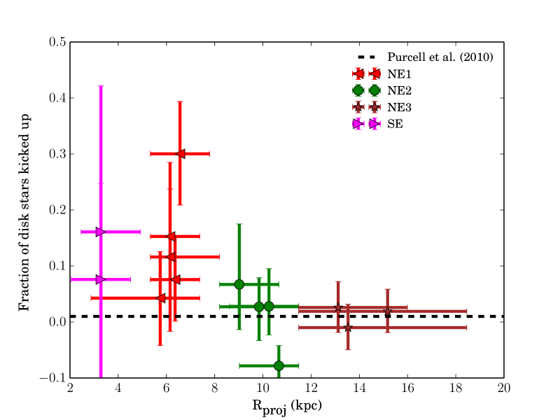
Figure 14.— Fraction of disk-like population that must be dynamically hot in order to simultaneously fit the LF and kinematics. Vertical error bars denote $1\sigma$ uncertainties and horizontal error bars denote the entire range of $R_{\rm proj}$ subtended by each subregion. The kicked up fraction in most of the subregions is consistent with, though systematically larger than, that predicted by Purcell et al. [2010] to result from a merger event at low impact angle with mass ratio 1:10.

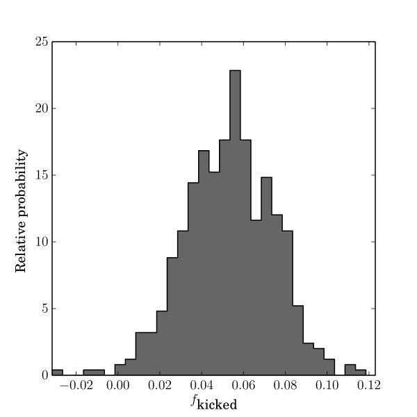
Figure 15.— PDF of $f_{\rm kicked}$, the fraction of disk stars that must be dynamically hot in order to simultaneously fit the LF and kinematics. This probability distribution is constructed from the 14 PDFs corresponding to the individual subregions, weighted by the number of stars in each subregion. The most probable value of $f_{\rm kicked}$ is 5.2%. The width of the distribution, a combination of spatial variation in $f_{\rm kicked}$ and uncertainty on the mean, is $1\sigma$ = $2.1\%$. The distribution is narrow enough that a model with zero kicked-up fraction is effectively excluded.

Our decomposition is of course limited by our choice of model, and there are many plausible parameterizations of the bulge, disk and halo SB profiles. For completeness, we consider the possibility that a modified SB model could eliminate the need for a kicked-up disk component. We attempt to fit the data with four different modified SB models, but none result in an acceptable fit to all three data sets.

First, we try fitting a model with a second exponential disk component with its own central intensity, ellipticity, scale length, and LF parameters. However, the most probable models in the posterior distribution are those with a single disk component.

We also try using a model with a single disk whose exponential scale length is allowed to change at a break radius $R_{\rm break}$ (that is, allowing for a Freeman type II or III profile). However, the likelihood values show no preference for a disk with a break.

Bulgeless disk galaxies can have SB profiles that deviate from pure exponential. We try fitting a model with a disk whose Sérsic index is a free parameter. The resulting PDF of the Sérsic index has a mean of $0.94\pm 0.4$ — that is, the disk is slightly more cored than a pure exponential. This decomposition does not reduce the required kicked-up fraction.

The BHB profile can be well fit by a halo component alone if the halo core radius is $\sim 3$ kpc [Williams et al., 2012]. We try fixing $R_{h}=3.0$ kpc, but this degrades the fit to the kinematics at large radii (regions NE2 and NE3) with minimal to no improvement at smaller radii.

The central region of M31 is complex, with multiple components including a classical bulge that dominates the SB within 0.2 kpc on the major axis, boxy bulge that dominates within 2.7 kpc, and bar that extends to at least 4.5 kpc [Beaton et al., 2007]. We allow for the possibility of multiple spheroidal components by fitting a model with two Sérsic bulges with unique central intensities, ellipticities, scale lengths, Sérsic indices, and LFs. However, the fit to the kinematics is not improved.

Finally, we try relaxing the assumption of a Sérsic bulge profile. The kinematics would be better fit if the bulge were more extended — if it had a shallower slope in the outer regions. However, the outer slope and inner slopes of a Sérsic profile are determined by the same parameter $n$, which in our case is completely constrained by the inner $\sim 0.7~{}\rm kpc$ (on the minor axis) where the bulge dominates the SB. We consider a modified Sérsic profile, whose inner and outer slopes are allowed to differ but whose shape reduces to a Sérsic when the slopes are the same. Even with this added flexibility, the data prefer models with near-Sérsic bulge profiles: small bulges nearly identical to those in Figure 10.

It is also possible that the excess dynamically hot population belongs to the virialized remnants of tidal debris. Dynamically cold substructure has been seen in M31’s halo and, to a smaller extent, in the portion covered by the PHAT survey; it is not unreasonable to suppose that the remnants from older satellite encounters contribute stars to the central portion of the galaxy. However, note that the debris would have to be old enough to have virialized (because it is dynamically hot), but have a significant fraction of young or intermediate-age stars (to have enough AGB stars to fill out the LF brightward of the TRGB). Analysis of cosmological simulations such as ERIS [Guedes et al., 2011] will provide insight into the relative contributions of young, virialized tidal debris and kicked-up disk stars in the inner halos of large spiral galaxies.

6.2. Relationship between bulge and halo

The location of the transition between M31’s bulge and halo has long been unclear. From images and SB decompositions [e.g., Courteau et al., 2011] the bulge appears to be relatively small, with a Sérsic index of around $2$ and an effective radius of around $1$ kpc. However, resolved stellar population studies have raised the possibility that the bulge may be much bigger. Deep optical HST CMDs of a minor-axis field at a projected radius of about 15 kpc ($\sim 12$ disk scale radii on the minor axis) revealed a broad spread in [Fe/H] ($\sim-1.5-0$) and age ($\sim 5-13$ Gyr) [Brown et al., 2003, 2006], more similar to the MW’s bulge than to its old, metal-poor inner halo. It appeared that either M31 has a large bulge or else its halo has had a much different formation history than the MW’s.

In Dorman et al. [2012], we showed that a significant fraction ($\sim 10-20\%$) of the stars in our kinematical sample belong to a dynamically hot population — presumably either the outer reaches of a centrally concentrated bulge or the inner portion of an extended halo. With kinematics alone, we were unable to distinguish between these two scenarios, but we are now in a position to show that the vast majority of these stars are associated with the halo.

Our decomposition indicates that the SB and LF profiles of the galaxy are much better fit by a small ($R_{b}=0.77\pm 0.03$ kpc) bulge. Figure 16 maps the fraction of spheroid SB due to the bulge. This fraction falls below 0.5 — that is, the halo dominates the spheroid SB — exterior to $R_{\rm proj}\sim 5.5$ kpc on the major axis. Nearly all of the SPLASH survey region falls in this halo-dominated region. As shown in § 6.1, some of these stars may have originated in the disk but have been dynamically heated to kinematically resemble halo members.

In Dorman et al. [2012], we found that the dynamically hot population rotates with $v/\sigma\sim 1/3$, significantly more slowly than the typical spiral galaxy bulge [Cappellari et al., 2007]. It is now clear that this is not necessarily a useful comparison, as the dynamically hot population is not physically associated with the bulge. A more relevant comparison would be to the “inner halo” of the MW, which rotates much more slowly than our dynamically hot population [Carollo et al., 2007, 2010]. It is possible that the accreted halo population in M31 resembles in the inner halo of the MW with almost no rotation, but the portion that originated in the disk has some residual rotation.

We can learn more about the relationship between the bulge and halo by comparing their SB profiles to the density profile of BHB stars, a reliable tracer of metal-poor populations. BHB stars have a mean metallicity of of [Fe/H]$\sim-1$, with only a small high-metallicity tail, and so are unlikely to have formed in more metal-rich subcomponents. Williams et al. [2012] combined star counts of CMD-selected BHB stars from the first two years of the PHAT survey. They showed that the density profile of BHB stars increases steeply interior to 10 kpc, but not as steeply as the density profile of RGB stars. Our results are qualitatively consistent with theirs. In Figure 17, we compare our halo SB profile and total SB profile (combined halo, bulge, and disk) to the BHB profile of Williams et al. [2012], scaling our SB profiles to match the BHB counts at $R=20~{}\rm kpc$. The BHB/SB ratio (which should trace the BHB/RGB ratio) increases with radius, as found in Williams et al. [2012].

However, our halo core radius is large enough that the halo alone cannot account for the BHB density interior to $10$ kpc. The disk (and possibly the bulge) must supplement the metal-poor population of the halo. Williams et al. [2012] argued that it was unlikely that a significant portion of the BHB stars belonged to the disk, in part because the kinematically-derived disk fraction in a field at $R=9$ kpc on the minor axis – where there were many BHB stars – was no more than $10\%$. However, we now know two reasons that this disk fraction may have been an underestimate. First, the SPLASH target selection strategy preferentially chooses spheroid stars over disk stars, underestimating the disk fraction by a factor of $1.6$ on the minor axis. Second, some fraction of the true disk stars may have been kicked up so that a kinematical decomposition grouped them with the halo. The metallicity distribution of the disk then is likely quite broad: some stars belong to a metal-poor BHB population, while the faint break magnitude of the disk LF indicates a contribution from stars with solar or supersolar metallicities.

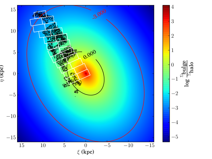
Figure 16.— Map of the relative contribution of the bulge to the spheroid SB. The bulge dominates over the halo in the central 5.5 kpc, but its surface brightness quickly falls off at larger radii. The spectroscopic sample (black dots) falls almost entirely in the region where the spheroid light is dominated by the halo; the dynamically hot stars are more likely to be associated with the halo than the bulge.

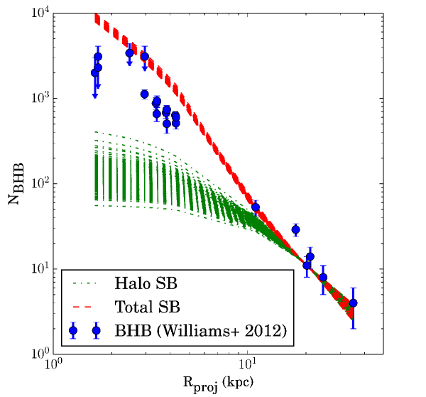
Figure 17.— Comparison between counts of blue horizontal branch (BHB; blue dots) stars, presumed to trace the metal-poor population [Williams et al., 2012], and the most probable halo profile from our decomposition (green dot-dashed lines), scaled to match the BHB counts at 20 kpc. One line is drawn for each of 256 points from the posterior probability distribution, so that the colored regions approximate the entire allowed (not $1\sigma$) region of parameter space. The power-law halo component cannot explain all of the BHB star counts; the bulge and/or the disk must contain a significant metal-poor population. The ratio of BHB counts to SB (red lines) increases with radius.

6.3. Radial Gradient in the Disk LF

As shown in Table 2, Figure 19 and Figure 20, the radial gradient parameters in the disk LF are exclusively nonzero.

To show that a radial gradient is required to simultaneously fit all three data sets, we run a test decomposition with a constant disk LF. The resulting fit to the LF is quite poor (median reduced $\chi^{2}=70$ including only observational uncertainties). Figure 18 shows the fits in a representative sample of three subregions. Most noticeably, the model predicts a number density that is too high at small radii and too low at large radii. The uncertainty parameter on the LF is driven high in an attempt to resolve the tension between the model and data, inflating the effective uncertainty beyond the Poisson uncertainty. In contrast, when we allow for a radial gradient, the LF uncertainty parameter can be very small, and the structural parameters and the fit to the kinematics are unaffected (see Figure 11).

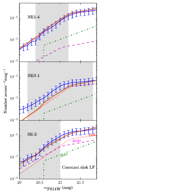
Figure 18.— Same as Figure 11, assuming a constant disk LF shape. The blue error bars, the quadrature sum between the Poisson uncertainties and the uncertainty parameter, have been significantly inflated relative to those in Figure 11 in an attempt to reduce the tension between the data and this model. A radial gradient in the disk LF does a much better job of fitting the LF data without affecting the fits to the SB or kinematical data.

It is not surprising that there is a radial gradient in the LF of M31’s stellar disk. Such a variation could be caused by either an age or metallicity gradient, either of which is plausible: HII region abundance estimates suggest that there may be a small metallicity gradient within M31’s (gas) disk [e.g., Sanders et al., 2012, Zurita & Bresolin, 2012], while inside-out disk formation and/or radial migration could induce an age gradient.

As discussed earlier in the paper, the break magnitude of the TRGB can be used as a proxy for metallicity: for populations with $\textrm{[Fe/H]}\gtrsim-1$, the TRGB is much more sensitive to metallicity than age, becoming fainter as metallicity increases. The shapes of the LFs in Figure 12 illustrate the trend from higher metallicity at low radius (red curves) to lower metallicity at high radius (orange curves). The same trend – metal abundance that decreases with radius – seen in M31 disk PNe [Sanders et al., 2012, Kwitter et al., 2011] and HII regions [Sanders et al., 2012, Zurita & Bresolin, 2012]. At large radii, the average metallicity of the disk is similar to that of the bulge, but still higher than that of the halo.

Note that this gradient exists in the old, smooth stellar disk; it does not reflect (and thus is not biased by) the sharp changes in stellar population found in the narrow star-forming rings. Recall that we excluded from the PHAT LF every star that fell within a $25\times 25~{}{\rm pc}^{2}$ pixel with a reddening $A_{v}>1.0$; as shown in the middle panel of Figure 5, this cut effectively removes stars in the star-forming rings. In addition, we have cut out the few remaining stars blue enough to still be on the young, massive main sequence.

7. Summary

We have presented the first structural decomposition of a large spiral galaxy using simultaneous SB, LF, and kinematical constraints. We have used Bayesian inference to find the probability distribution functions of 32 parameters describing the surface brightness profile and LF of each structural subcomponent. We have found:

1. The structural parameters we measure are consistent with previous measurements. On average, the old stellar disk is more highly inclined and its major axis PA is larger than measured from isophotal SB fitting.

2. A decomposition including a Sérsic bulge, power-law halo, exponential disk and constant shapes to the bulge, halo, and disk LFs cannot simultaneously well fit the SB, LF, and kinematical data. The model poorly predicts the number density of bright stars and overestimates the disk fraction in most subregions.

3. The high kinematically-derived spheroid fractions can be explained if some spatially dependent fraction (between $1\%$ and $30\%$) of the dynamically hot component is comprised of “kicked-up” disk stars. This kicked-up population has a disklike SB profile and disklike LF, but spheroidlike kinematics ($\sigma_{v}\sim 150~{}\rm km~{}s^{-1}$).

4. In the I band, the halo is brighter than the bulge exterior to $R=5.5~{}\rm kpc$ on the major axis.

5. Comparison to BHB stars, a tracer of the metal-poor population, indicates that the disk metallicity distribution has a low-metallicity tail.

6. A SB decomposition including a radially varying disk LF improves the fit to the observed LF and does not affect the structural parameters.

Table 2Model Parameters

Parameter	Description	Units	Allowed Range	Results
$\mu_{d}$	Disk central SB	mag	$0<\mu_{d}<\infty$	$18.901^{+0.032}_{-0.031}$
$R_{d}$	Disk scale length	kpc	$0<R_{d}<\infty$	$5.76^{+0.101}_{-0.113}$
$\epsilon_{d}$	Disk ellipticity	1	$0<\epsilon_{d}<1$	$0.725^{+0.005}_{-0.005}$
$\mu_{b}$	Bulge SB at $R_{e}$	mag	$0<\mu_{b}<\infty$	$17.849^{+0.066}_{-0.066}$
$R_{b}$	Bulge half-light radius	kpc	$0<R_{b}<\infty$	$0.778^{+0.03}_{-0.028}$
$n_{b}$	Bulge Sersic index	1	$0<n_{b}<10$	$1.917^{+0.082}_{-0.081}$
$\epsilon_{b}$	Bulge ellipticity	1	$0<\epsilon_{b}<1$	$0.277^{+0.011}_{-0.011}$
$\mu_{h}$	Halo central intensity	mag	$0<\mu_{h}<\infty$	$24.18^{+0.295}_{-0.328}$
$R_{h}$	Halo scale radius	kpc	$0<R_{h}<\infty$	$10.631^{+2.459}_{-2.034}$
$\epsilon_{h}$	Halo ellipticity	1	$0<\epsilon_{h}<1$	$0.215^{+0.109}_{-0.12}$
$\alpha_{h}$	Halo power-law slope	1	$0<\alpha_{h}<\infty$	$2.508^{+0.232}_{-0.199}$
PA	Major axis PA	degrees	$0<\textrm{PA}<180$	$6.632^{+0.459}_{-0.511}$
$y_{d0}$	Disk # density/SB, $R_{\textrm{disk}}$ = 1 kpc	$10^{5}\textrm{N}/\textrm{arcsec}^{2}$/mag	$0<y_{d0}<\infty$	$1.93^{+4.00}_{-3.90}$
$p_{d0}$	Disk LF bright-end slope, $R_{\textrm{disk}}$ = 1 kpc	log(N)/mag	$0<p_{d0}<\infty$	$4.519^{+0.313}_{-0.267}$
$q_{d0}$	Disk LF faint-end slope, $R_{\textrm{disk}}$ = 1 kpc	log(N)/mag	$0<q_{d0}<\infty$	$2.012^{+0.826}_{-0.843}$
$l_{d0}$	Disk LF break magnitude, $R_{\textrm{disk}}$ = 1 kpc	mag	$20<l_{d0}<22$	$21.782^{+0.146}_{-0.209}$
$\delta y_{d}$	Radial gradient in disk # density/SB	N/$\textrm{arcsec}^{2}$/mag/ln(kpc)	$-\infty<\delta y_{d}<\infty$	$0.001^{+0.0}_{-0.0}$
$\delta p_{d}$	Radial gradient in disk LF bright-end slope	log(N)/mag/ln(kpc)	$-\infty<\delta p_{d}<\infty$	$-0.21^{+0.083}_{-0.06}$
$\delta q_{d}$	Radial gradient in disk LF faint-end slope	log(N)/mag/ln(kpc)	$-\infty<\delta q_{d}<\infty$	$-0.777^{+0.111}_{-0.134}$
$\delta l_{d}$	Radial gradient in disk LF break magnitude	mag/ln(kpc)	$-\infty<\delta l_{d}<\infty$	$-0.672^{+0.321}_{-0.308}$
$y_{b}$	Bulge # density/SB	N/$\textrm{arcsec}^{2}$/mag	$0<y_{b}<\infty$	$0.007^{+0.002}_{-0.001}$
$p_{b}$	Bulge LF bright-end slope	log(N)/mag	$0<p_{b}<\infty$	$2.494^{+0.405}_{-0.38}$
$q_{b}$	Bulge LF faint-end slope	log(N)/mag	$0<q_{b}<\infty$	$0.424^{+0.434}_{-0.307}$
$l_{b}$	Bulge LF break magnitude	mag	$20<l_{b}<22$	$21.125^{+0.144}_{-0.189}$
$y_{h}$	Halo # density/SB	N/$\textrm{arcsec}^{2}$/mag	$0<y_{h}<\infty$	$0.014^{+0.004}_{-0.003}$
$q_{h}$	Halo LF faint-end slope	log(N)/mag	$0<q_{h}<\infty$	$1.592^{+0.301}_{-0.351}$
$l_{h}$	Halo LF break magnitude	mag	$20.3<l_{h}<22$	$20.805^{+0.046}_{-0.052}$
$\epsilon_{\textrm{LF}}$	LF uncertainty parameter	1	$0<\epsilon_{\textrm{LF}}<\infty$	$0.129^{+0.008}_{-0.007}$
$\epsilon_{\textrm{Choi}}$	Uncertainty on Choi SB data	1	$0<\epsilon_{\textrm{Choi}}<2$	$0.086^{+0.005}_{-0.005}$
$\epsilon_{\textrm{Gilbert}}$	Uncertainty on Gilbert SB data	1	$0<\epsilon_{\textrm{Gilbert}}<2$	$0.815^{+0.155}_{-0.124}$
$\epsilon_{\textrm{PvdB}}$	Uncertainty on PvdB SB data	1	$0<\epsilon_{\textrm{PvdB}}<2$	$0.577^{+0.7}_{-0.333}$
$\epsilon_{\textrm{Irwin}}$	Uncertainty on Irwin SB data	1	$0<\epsilon_{\textrm{Irwin}}<2$	$0.086^{+0.005}_{-0.005}$

8. Acknowledgments

We thank Stephane Courteau, Alis Deason, Dimitrios Gouliermis, James Guillochon, Katherine Hamren, Antonela Monachesi, and Annalisa Pillepich for helpful discussions and feedback. PG and CD acknowledge NSF grants AST-0607852 and AST-1010039 and NASA grant HST-GO-12055. KG acknowledges Hubble Fellowship grant 51273.01 awarded by the Space Telescope Science Institute, which is operated by the Association of Universities for Research in Astronomy, Inc., for NASA, under contract NAS 5-26555. Additionally, CD was supported by a NSF Graduate Research Fellowship.

We acknowledge the very significant cultural role and reverence that the summit of Mauna Kea has always had within the indigenous Hawaiian community. We are most fortunate to have the opportunity to conduct observations from this mountain.

Appendix A Spectroscopic Data

The details of the spectroscopic target selection and observation are given in Dorman et al. [2012]. However, here in Table 3, we describe the five additional slitmasks that were observed with Keck/DEIMOS in November 2011 and therefore were not included in Dorman et al. [2012].

All of the targets on these five masks were candidate RGBs identified on the basis of the optical CMD from the PHAT survey.

Table 3Keck/DEIMOS Multiobject Slitmask Exposures from Fall 2011

Mask	Observation	$\alpha$ [J2000]	$\delta$ [J2000]	P.A.	$t_{\rm{exp}}$	Seeing	No. of	No. of Usable	No. of Usable
Name	Date (UT)	(h m s)	(∘ ′ ′′)	(∘)	(sec)	FWHM	Slits	Target Velocities	Velocities of
								(Success Rate)	Serendipitously Detected
									Stars
mctF	2011 Nov 23	00 44 24.00	$+$41 36 00.0	$-$30.0	2900	$0\farcs 6$	246	179 (73%)	47
mctG	2011 Nov 23	00 45 53.03	$+$41 42 05.1	$+$25.0	2900	$0\farcs 5$	259	207 (80%)	24
mctJ	2011 Nov 24	00 45 10.80	$+$41 55 48.0	$+$35.0	3600	$0\farcs 6$	253	182 (72%)	18
mctK	2011 Nov 24	00 46 46.85	$+$42 13 35.3	$+$45.0	3400	$0\farcs 8$	270	208 (78%)	10
mctL	2011 Nov 23	00 46 19.97	$+$42 14 05.2	$-$65.0	3680	$1\farcs 0$	257	182 (71%)	7
Total:							1285	958 (75%)	106

Appendix B MCMC Sampler

To estimate the marginalized posterior probability function of the model parameters, we draw samples from the distribution $P$ (Equation 29) using a Markov chain Monte Carlo sampler [MCMC; Bishop, 2003, Gelman et al., 2003, MacKay, 2003, Press et al., 2007]. MCMC algorithms offer a method of efficiently drawing unbiased samples from any distribution that can be evaluated for a given set of parameters. In this case, the distribution of interest is the posterior probability which is—up to an unimportant normalization constant—the product of the likelihood function (Equation 29) and the prior distributions over the parameters (which we choose to be flat for all parameters). Drawing samples from this distribution is equivalent to drawing a representative sampling of physical models that are consistent with the data and the uncertainties.

The most popular class of MCMC algorithms are based on the Metropolis–Hastings (M–H) method [e.g., MacKay, 2003]. For this project we use a more efficient ensemble sampler called emcee that takes advantage of an affine-invariant proposal distribution in order to sample efficiently even in arbitrarily covariant parameter spaces [Goodman & Weare, 2010, Foreman-Mackey et al., 2013]. In many cases, emcee requires many fewer computations than required by a standard M–H algorithm to draw the same number of independent samples from a distribution. The advantage comes from the fact that emcee uses an affine-invariant algorithm, meaning that it performs equally well regardless of the covariance between parameters. If a M–H chain is to perform well, the proposal distribution—which generally has $\sim D^{2}$ free parameters, where D is the number of dimensions in the problem—must be tuned to match the covariances in the target density using a computationally expensive “burn-in” phase. In contrast, emcee has only 2 free parameters and the proposal density adaptively fits the target density without any fine tuning. This is achieved by simultaneously evolving $K$ coupled MCMC chains or “walkers”. Each walker produces unbiased samples from the target distribution but the proposal distribution for each walker is determined by the current positions of all the other walkers. For more information about this algorithm and the implementation details, see the discussion in Foreman-Mackey et al. [2013].

For this project, we use 256 walkers and keep the emcee proposal scale—called $a$ in Foreman-Mackey et al. [2013] —at the default value of 2. Each MCMC run is composed of $\sim 10,000$ “burn-in” steps for each walker and then $100$ production steps. The results given in the paper are based on the $256\times 20=51,200$ samples produced after burn-in. In particular, the final column in Table 2 reports the sample mean and standard deviation of the parameters in the production chain.

Appendix C Parameter Distributions

Figures 19 and 20 show the 1D posterior probability distributions of all model parameters using samples from the last $20$ steps of the MCMC chain. Each distribution is normalized to an area of 1 for display purposes. Descriptions of parameters are given in Table 2.

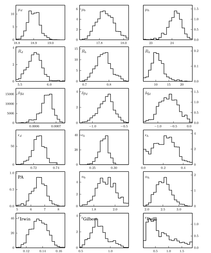
Figure 19.— Posterior probability distributions of each parameter, as drawn from the last 20 steps of the MCMC chain. Units are given in Table 2. With the exception of the third row, parameters describing the disk, bulge, and halo are shown in the left, middle, and right columns, respectively.

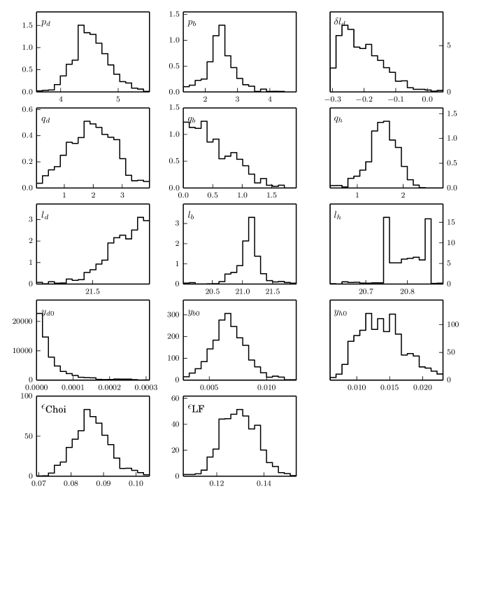
Figure 20.— Figure 19, continued.