Circular handle decompositions of free genus one knots

Abstract.

We determine the structure of the circular handle decompositions of the family of free genus one knots. Namely, if $k$ is a free genus one knot, then the handle number $h(k)=$ 0, 1 or 2, and, if $k$ is not fibered (that is, if $h(k)>0$), then $k$ is almost fibered. For this, we develop practical techniques to construct circular handle decompositions of knots with free Seifert surfaces in the 3–sphere (and compute handle numbers of many knots), and, also, we characterize the free genus one knots with more than one Seifert surface. These results are obtained through analysis of spines of surfaces on handlebodies. Also we show that there are infinite families of free genus one knots with either $h(k)=1$ or $h(k)=2$.

1. Introduction

In the study of the topology of a given 3–manifold, $M$, it has been useful to consider regular real-valued Morse functions $f:M\rightarrow\mathbb{R}$ where $M$ has some smooth structure. A regular real-valued Morse function on $M$ corresponds to a handle decomposition of $M$ of the form $M=b_{0}\cup B_{1}\cup P_{1}\cup\cdots\cup B_{r}\cup P_{r}\cup b_{3}$ where $b_{0}$ is a collection of 0-handles, $B_{j}$ is a collection of 1–handles, $P_{j}$ is a collection of 2–handles, and $b_{3}$ is a collection of 3–handles, in such a way that the $i$–handles of the decomposition are neighbourhoods of the critical points of index $i$ of the Morse function ($j=1,\dots,r$, and $i=0,1,2,3$). In a celebrated paper ([14]), it is introduced the concept of thin position for 3–manifolds; the idea is to build the manifold as described above (that is, step by step: adding to the set $b_{0}$ the set $B_{1}$, and then adding $P_{1}$, and then adding $B_{2}$, and so on) with a sequence of selected sets of 1–handles and sets of 2–handles chosen to keep the boundaries of the intermediate steps as simple as possible.

Now if a 3–manifold $M$ satisfies $H^{1}(M;\mathbb{Q})\neq 0$, then there are essential (non-nulhomotopic) regular Morse functions $f:M\rightarrow S^{1}$, and one can always find this kind of functions having only critical points of index 1 and 2 (see Section 2.2). Such a function corresponds to a circular handle decomposition $M=F\times[0,1]\cup B_{1}\cup P_{1}\cup\cdots\cup B_{r}\cup P_{r}$ where $F$ is a properly embedded surface in $M$, $B_{j}$ is a collection of 1–handles, and $P_{j}$ is a collection of 2–handles (the handles are glued along, say, $F\times\{1\}$), and, as above, the set of $i$–handles of the decomposition corresponds to the critical points of index $i$ of the Morse function. With this kind of circular handle decompositions we may also require that the intermediate steps be as simple as possible: that requirement acquires the notion of thin position for circular handle decompositions. The existence of these decompositions gives rise to numerical topological invariants such as the (circular) handle number, $h(M)=\sum_{1=1}^{r}\#(B_{i})$ where the sum $\sum\#(B_{i})$ is minimal among all circular handle decompositions; also, when the decomposition is in thin position, we obtain the circular width, $cw(M)$ (See Section 2.4).

Outstanding examples of manifolds that admit circular handle decompositions, are the exteriors of links in $S^{3}$. In this case the interesting intermediate surfaces in the decomposition are Seifert surfaces for the given link (these intermediate surfaces have no closed components, and, if the decomposition is in thin position, they are a sequence of Seifert surfaces which are alternately incompressible and weakly incompressible. See [9], Theorem 3.2, where there is a statement for knots, but its proof works verbatim for links).

If the exterior of a link $\ell$ in $S^{3}$ admits a circular decomposition of the form $E(\ell)=F\times[0,1]\cup B_{1}\cup P_{1}$, and this decomposition is in thin position, we say that $\ell$ is an almost fibered link. One may regard the set of almost fibered knots as the set of knots with non-trivial simplest circular handle structure.

Thus, an interesting problem of this theory is: Determine the set of all almost fibered knots. We solve this problem for the family of free genus one knots. In fact we show that all free genus one knots are almost fibered (Theorem 6.7).

Also it is interesting to find explicit constructions of circular handle decompositions of the exterior of a given link which are minimal (that is, that realize the handle number), or that are in thin position. In [2], although in other context, explicit minimal circular handle decompositions of the exterior of the 250 knots in Rolfsen’s table are given. Of these knots, 117 are fibered, and 132 have handle number one. As far as we know, there are no other previously published explicit constructions of circular handle decompositions of exteriors of links in the 3–sphere.

As mentioned above, in this paper we are interested mainly in the circular handle structures of the family of free genus one knots:

In the first part of this work (Section 3) we develop techniques to construct explicit circular decompositions of link exteriors for links that admit a free Seifert surface; these decompositions are interesting, of course, when the free Seifert surface used in the construction is of minimal genus for the link. The information needed to construct these decompositions for the exterior of a given link is encoded in some spine of a free Seifert surface of the link. In this sense, the techniques developed in Section 3 (and through all this paper) could be regarded as elements for a possible theory of spines of surfaces on handlebodies that might be worthy of consideration. As applications we construct minimal circular decompositions for all rational knots and links and, also, for a family of pretzel knots, namely, pretzel knots of the form $P(\pm 3,q,r)$ with $|q|,|r|$ odd integers $\geq 3$. These circular decompositions for both families of links are all minimal and have handle number one; they are also in thin position, giving also the circular width of each link considered. This last family gives examples of non-fibered knots whose handle number is strictly less than their tunnel number (Remark 3.10). Also, it is shown that free genus one knots have handle number $\leq 2$ (Corollary 3.5).

Secondly (Section 4), we construct circular handle decompositions for the exteriors of all pretzel knots of the form $P(p,q,r)$ with $|p|,|q|,|r|$ odd integers $\geq 5$, and we show that these decompositions are minimal with handle number two (Theorem 4.1), and are also in thin position, giving the circular width equal to 6 for each of these knots. These examples answer a question posed in [11] (Remark 4.5).

Next, in Section 5, we give a characterization of the free genus one knots that admit at least two different (non-parallel) Seifert surfaces of genus one. This characterization is given in terms of the existence of a special spine for the given genus one free Seifert surface of the knot (see Theorem 5.2).

Using the characterization given in Section 5 we show, in the final part of this work, that all (non-fibered) free genus one knots are almost fibered (Theorem 6.7).

It follows from the proof of Theorem 6.7, that the free genus one knots with handle number two have a unique minimal genus Seifert surface (that is, free genus one knots with at least two genus one Seifert surfaces have handle number one). It is an interesting open problem to determine the family of free genus one knots with handle number two.

2. Preliminaries

Unless explicitly stated, we will use the word ‘knot’ for a knot or a link in $S^{3}$. That is, we will emphasize connectedness if needed. Otherwise, we will admit non-connected knots.

Let $X$ be a manifold and let $Y\subset X$ be a sub-complex. We write $E(Y)=\overline{X-\mathcal{N}(Y)}$ for the exterior of $Y$ in $X$ where $\mathcal{N}(Y)$ is a regular neighbourhood of $Y$ in $X$.

Let $X$ be a manifold and let $Y\subset X$ be a properly embedded submanifold. $Y$ is called $\partial$–parallel in $X$, or parallel into $\partial X$, if there is an embedding $e:(Y,\partial Y)\times I\rightarrow(X,\partial X)$, such that $e_{0}:Y\rightarrow Y$ is the identity, and $e_{1}(Y)\subset\partial X$. If $Y$ is $\partial$–parallel in $X$ with embedding $e:(Y,\partial Y)\times I\rightarrow(X,\partial X)$, then the submanifold $e(Y\times I)$ is called a $\partial$–parallelism for $Y$. Notice that if $Y$ is disconnected with components $Y_{1},\dots,Y_{n}$, and $Y$ is $\partial$–parallel in $X$ with a $\partial$–parallelism $W$, then $W$ is a disjoint union of $\partial$–parallelisms $W_{1},\dots,W_{n}$ for $Y_{1},\dots,Y_{n}$, respectively.

2.1. Seifert Surfaces

Let $k\subset S^{3}$ be a knot, and let $F$ be a Seifert surface for $k$; that is, $F$ is an orientable surface and $\partial F=k$. Then, by drilling out a small neighbourhood, $\mathcal{N}(k)$, of $k$, the surface $\widehat{F}=F\cap E(k)$ is a properly embedded surface in $E(k)$, the exterior of $k$ in $S^{3}$, and one may assume that $\partial\widehat{F}$ is parallel to $k$ in $\mathcal{N}(k)$. Usually, we identify $F$ with $\widehat{F}$; but, more appropriately, we start with $F\subset E(k)$ a Seifert surface for $k$. Seifert surfaces may be disconnected, but they are not allowed to contain closed components. The genus $g(k)$ of a knot $k$ is the minimal genus among all Seifert surfaces for $k$.

A surface $F\subset S^{3}$ is called free if $E(F)$ is a handlebody. The free genus of a knot $k$, $g_{f}(k)$, is the minimal genus among all free Seifert surfaces for $k$.

In this work we will be interested mainly in free genus one knots.

2.2. Handle decompositions of rel $\partial$ Cobordisms

Let $W$ be a cobordism rel $\partial$ between surfaces with no closed components, $\partial_{+}W$ and $\partial_{-}W$. A moderate handle decomposition of $W$ is a decomposition of the form $W\cong\partial_{+}W\times I\cup(\textrm{1--handles})\cup(\textrm{2--handles})$. Given $W$, a cobordism rel $\partial$ between surfaces with no closed components, $\partial_{+}W$ and $\partial_{-}W$, it is easy to find a moderate decomposition as above by considering a triangulation of the exterior $E(\partial_{+}W)=\overline{W-\mathcal{N}(\partial_{+}W)}$.

Given a cobordism $W$ and a moderate handle decomposition for $W$, one can find a regular Morse function $f:W\rightarrow I$ which realizes the handle decomposition of $W$. That is, $f$ only has critical points of index 1 and 2, and neighbourhoods of the critical points of $f$ correspond to the 1 and 2–handles of $W$, and the preimage of each regular value of $f$ is a properly embedded surface in $W$. We will call such a Morse function a moderate Morse function (see [11]).

2.3. Circular decompositions

Let $k$ be a knot in $S^{3}$. Since $H_{1}(E(k))$ is a free Abelian group of positive rank, we can always find an essential (non-nulhomotopic) moderate Morse function $f:E(k)\rightarrow S^{1}$. Any such Morse function, as in Subsection 2.2, induces a decomposition

$$E(k)=(F\times I)\cup B\cup P$$

where $F\subset E(k)$ is a Seifert surface for $k$, $B$ is a set of $n$ 1–handles glued along, say, $F\times\{1\}$, and $P$ is a set of the same number, $n$, of 2–handles glued along the same side.

We call such a decomposition a circular handle decomposition of $E(k)$ based on $F$, and write $h(F)=n$, the handle number of $F$, where $n$ is the minimal number of 1–handles among all circular handle decompositions of $E(k)$ based on $F$. The circular handle number of $k$, or simply the handle number of $k$, $h(k)$, is the minimal $h(F)$ among all Seifert surfaces $F\subset E(k)$. Notice that $h(k)=0$ if and only if $k$ is a fibered knot.

By rearranging the critical points of a moderate Morse function $f:E(k)\rightarrow S^{1}$, we can thin a circular handle decomposition of $E(k)$:

$$E(k)=(F\times I)\cup B_{1}\cup P_{1}\cup B_{2}\cup P_{2}\cup\cdots\cup B_{\ell}\cup P_{\ell}$$

where $B_{i}$ is a set of 1–handles glued along $F\times\{1\}$, and $P_{i}$ is a set of 2–handles, $i=1,\dots,\ell$ (of course, it is not always possible to thin a given circular handle decomposition).

For $i=1,\dots,\ell$, the set $W_{i}=(F\times[\frac{1}{2},1])\cup B_{1}\cup P_{1}\cup\cdots\cup B_{i}$ gives a moderate handle decomposition for the rel $\partial$ cobordism $W_{i}$ with $\partial_{+}W_{i}=F\times\{\frac{1}{2}\}$. Write $S_{i}=\partial_{-}W_{i}$. Now we define

$$c(S_{i})=\sum_{j=1}^{n_{i}}\left(1-\chi(G_{i,j})\right)$$

where $\chi$ stands for Euler characteristic, and $G_{i,1},\dots,G_{i,n_{i}}$ are the components of $S_{i}$ (Notice that there are no closed components of $S_{i}$ for, $F$ has no closed components and the handle decomposition is moderate). Order the surfaces $S_{\sigma(1)},S_{\sigma(2)},\dots,S_{\sigma(\ell)}$ in such a way that $c(S_{\sigma(i)})\geq c(S_{\sigma(i+1)})$ for $i=1,\dots,\ell-1$, where $\sigma$ is a permutation in the symbols $1,\dots,\ell$. Then the circular width of this decomposition is the tuple $(c(S_{\sigma(1)}),c(S_{\sigma(2)}),\dots,c(S_{\sigma(\ell)}))$. The circular width of $k$, $cw(k)$, is the minimal circular width, with respect to lexicographic order, among all thinned circular decompositions of $E(k)$ based on all possible Seifert surfaces for $k$.

Let $k\subset S^{3}$ be a knot such that its circular width has the form $cw(k)=(n)$. Then we write $cw(k)=n$, or $cw(k)\in\mathbb{Z}$. If $k$ is a non-fibered knot and $cw(k)\in\mathbb{Z}$, then $k$ is said to be an almost fibered knot.

Remark 2.1.

Equivalence of knots. Let $k,\ell\subset S^{3}$ be two knots. If the pairs $(S^{3},k)$ and $(S^{3},\ell)$ are homeomorphic, then their exteriors also are homeomorphic, $E(k)\cong E(\ell)$; and therefore, the exteriors of $k$ and $\ell$ have homeomorphic handle decompositions. We regard two knots as being equivalent if their corresponding pairs are homeomorphic.

Remark 2.2.

Construction of circular decompositions. To describe or, rather, to actually construct a decomposition

$$E(k)=(F\times I)\cup B\cup P$$

where $B$ is a set of 1–handles, and $P$ is a set of 2–handles, it is convenient to write

$$\textstyle E(k)=(F\times[\frac{1}{2},1])\cup B\cup P\cup(F\times[0,\frac{1}{2}]).$$

Then to obtain (describe) this circular decomposition we can either

1. Start with a regular neighbourhood $\mathcal{N}(F)$ of $F$ in $E(k)$. Then add a number of 1–handles to $\mathcal{N}(F)$ (the elements of $B$) on one side, say $F\times\{1\}$, and then add the same number of 2–handles (the elements of $P$) on the same side.

   The complement of the union above is a regular neighbourhood of $F\times\{0\}$ in $E(k)$. Or

2. Start with $E(F)$, the exterior of $F$ in $E(k)$. Then drill a number of 2–handles (the elements of $B$) out of $E(F)$. Now drill the same number of 1–handles (the elements of $P$) out of $E(F)$.

   Here one should be careful that the drilled out 2–handles intersect $\partial E(F)$ on the same side, say $F\times\{1\}$, and that the following drilled out 1–handles intersect the remaining boundary of $E(F)$ on the same side.

   The result of this drilling is a regular neighbourhood of $F\times\{0\}$ in $E(k)$.

Of course, in (1) above, ‘$\mathcal{N}(F)$’ stands for $F\times[\frac{1}{2},1]$, and in (2), ‘$E(F)$’ stands for the exterior $\overline{E(k)-F\times[\frac{1}{2},1]}$. To describe a thinned circular decomposition, one proceeds similarly, but now there will be several steps. Note that, in this kind of decomposition, a thinned decomposition, the number of 1–handles and the number of 2–handles at each step are not necessarily the same.

We emphasize that the main use of the program outlined in (1) is to describe an explicit circular handle decomposition of some given example.

Remark 2.3.

Decompositions of non almost fibered knots. Now start with a circular decomposition

$$\textstyle E(k)=(F\times[\frac{1}{2},1])\cup B_{1}\cup P_{1}\cup B_{2}\cup P_{2}\cup\cdots\cup B_{\ell}\cup P_{\ell}\cup(F\times[0,\frac{1}{2}])$$

which realizes $cw(k)$, the circular width of $k$. For $i=1,\dots,\ell$, the set $V_{i}=(F\times[\frac{1}{2},1])\cup B_{1}\cup P_{1}\cup\cdots\cup B_{i}\cup P_{i}$ gives a moderate handle decomposition for the rel $\partial$ cobordism $V_{i}$ with $\partial_{+}V_{i}=F\times\{\frac{1}{2}\}$. Write $T_{i}=\partial_{-}V_{i}$. Then the $\ell$ disjoint surfaces $T_{1},T_{2},\dots,T_{\ell}=F$ are incompressible in $E(k)$ and are non-parallel by pairs (see [9], Theorem 3.2. As noted in the Introduction, the theorem also holds for non-connected knots). That is,

If $k$ is non fibered and not an almost fibered knot, then $k$ has at least two non-parallel incompressible Seifert surfaces.

Remark 2.4.

Decompositions of pairs. Let $k\subset S^{3}$ be a knot with Seifert surface $F\subset E(k)$. There is a copy of $F$, $F_{0}\subset\partial E(F)$, such that $E(F)$ is a cobordism rel $\partial$ between $F_{0}=\partial_{+}E(F)$ and $\partial_{-}E(F)$. We commit an abuse of notation by identifying $F$ with $F_{0}$. To find a circular decomposition of $E(k)$ based on $F$ is the same as finding a moderate handle decomposition of the rel $\partial$ cobordism $E(F)$. A handle decomposition of the pair $(E(F),F)$ is, by definition, a handle decomposition of the rel $\partial$ cobordism $E(F)$.

Now let $\ell\subset S^{3}$ be another knot with Seifert surface $G\subset E(\ell)$. If there is a homeomorphism of pairs $(E(F),F)\cong(E(G),G)$, then the handle decompositions of the pairs $(E(F),F)$ and $(E(G),G)$ (as well as those of $E(F)$ and $E(G)$ as rel $\partial$ cobordisms) are in 1-1 correspondence via the given homeomorphism. That is:

To find circular decompositions of $E(k)$ based on $F$, we need only to construct moderate handle decompositions of the homeomorphism class of the pair $(E(F),F)$. In particular, it is not necessary to regard $E(F)$ as embedded in $S^{3}$.

This remark is very helpful in the search of circular decompositions.

2.4. Spines

Let $X$ be either a handlebody or a surface with boundary. A spine of $X$ is a graph $\Gamma\subset X$ such that $X$ is a regular neighbourhood of $\Gamma$. In this work we mainly consider spines of the form $\Gamma\cong\bigvee_{i=1}^{n}S^{1}$, a wedge of circles. We write $\Gamma=a_{1}\vee\cdots\vee a_{n}$ to emphasize the circles involved, and we assume that the curves $a_{i}$ carry a given orientation. Notice that it is allowed for $\Gamma$ to be a single simple closed curve.

Let $k\subset S^{3}$ be a knot, and let $F\subset E(k)$ be a Seifert surface for $k$. A regular neighbourhood $\mathcal{N}(F)$ of $F$ in $E(k)$ admits a product structure $\mathcal{N}(F)=F\times I$ where $\partial F\times I=\mathcal{N}(k)\cap\mathcal{N}(F)$. A spine $\Gamma\subset F\times\{0\}$, $\Gamma\cong\bigvee_{i=1}^{n}S^{1}$, is also a spine for $\mathcal{N}(F)$, and the graph $\Gamma$ induces a product structure $\mathcal{N}(F)=G\times I$, where, say, $G\times\{0\}$ is a regular neighbourhood of $\Gamma$ in $\partial\mathcal{N}(F)$ (here, of course, $G$ is isotopic to $F$ in $\partial\mathcal{N}(F)$). A spine $\Gamma\subset F\times\{0\}$ is also a graph $\Gamma\subset\partial E(F)$. A spine for $F$, $\Gamma\subset F\times\{0\}$ (or $\Gamma\subset F\times\{1\}$), is called a spine for $F$ on $\partial\mathcal{N}(F)$. Also, we say that $\Gamma$ is a spine for $F$ on $\partial E(F)$.

If $\Gamma$ is a spine for $F$ on $\partial E(F)$, and $G$ is a regular neighbourhood of $\Gamma$ in $\partial E(F)$, then a handle decomposition for the pair $(E(F),\Gamma)$ is, by definition, a handle decomposition for the pair $(E(F),G)$.

Let $\Gamma=a_{1}\vee\cdots\vee a_{n}$ be a spine for $F$ on $\partial E(F)$, and let $t(a_{i})$ be a Dehn twist on $F$ along the curve $a_{i}$. If $\widetilde{\Gamma}$ is the graph obtained from $\Gamma$ by replacing the curve $a_{j}$ by the curve $t(a_{i})(a_{j})$, then $\widetilde{\Gamma}$ is also a spine for $F$. The graph $\widetilde{\Gamma}$ is called the spine for $F$ obtained from $\Gamma$ by sliding $a_{j}$ along $a_{i}^{\pm 1}$ ($i,j\in\{1,\dots,g\}$).

Remark 2.5.

Notice that if $\widetilde{\Gamma}$ is another spine for $F$ on $\partial E(F)$, and $\widetilde{G}$ is a regular neighbourhood of $\widetilde{\Gamma}$ in $\partial E(F)$, then the pairs $(E(F),\Gamma)$ and $(E(F),\widetilde{\Gamma})$ usually are not homeomorphic, but the pairs $(E(F),F)$ and $(E(F),\widetilde{G})$ are homeomorphic. Thus:

To find circular decompositions of $E(k)$ based on $F$, we need only to construct moderate handle decompositions of the homeomorphism class of a pair $(E(F),\Gamma)$ for some spine $\Gamma$ for $F$ on $\partial E(F)$.

Remark 2.6.

Let $F\subset S^{3}$ be a connected orientable surface with boundary $k=\partial F$. If a spine $\Gamma$ for $F$ on $\partial\mathcal{N}(F)$ is also a spine for $E(F)$, then $k$ is a fibered knot with fiber $F$. Indeed, $E(F)$ is a handlebody (for it is an irreducible 3–manifold with connected boundary, and with free fundamental group), and both $\mathcal{N}(F)$ and $E(F)$ admit a product structure of the form $G\times I$, where $G$ is a regular neighbourhood of $\Gamma$ in $\partial\mathcal{N}(F)=\partial E(F)$.

2.5. Whitehead diagrams

Let $H$ be a genus $g$ handlebody, and let $x_{1},\dots,x_{g}$ be a system of meridional disks for $H$. The exterior $E(x_{1}\cup\cdots\cup x_{g})$ is a 3–ball with $2g$ fat vertices $x_{1},\bar{x}_{1},\dots,x_{g},\bar{x}_{g}$ on its boundary, where $x_{i}=x_{i}\times\{0\}$ and $\bar{x}_{i}=x_{i}\times\{1\}$ are the copies of $x_{i}$ in the product structure $\mathcal{N}(x_{i})=x_{i}\times I\subset H$, $i=1,\dots,g$.

There is a 1-1 correspondence between isotopy classes of systems of meridional disks $\{x_{1},\dots,x_{g}\}$ for $H$, and homotopy classes of spines of the form $a_{1}\vee\cdots,\vee a_{g}\subset H$ such that $\#(a_{i}\cap x_{i})=1$, and $a_{i}\cap x_{j}=\emptyset$ for $i\neq j$, $i,j=1,\dots,g$. It is convenient to commit an abuse of notation, and write both $\{x_{1},\dots,x_{g}\}$ for a meridional system of disks for $H$, and $\{x_{1},\dots,x_{g}\}$ for the corresponding basis of $\pi_{1}(H)$ represented by the curves $a_{1},\dots,a_{g}$ in the 1-1 correspondence above. Throughout this paper we adhere to this abuse of notation.

A graph $\Gamma=a_{1}\vee\cdots\vee a_{n}\subset\partial H$ intersects $E(x_{1}\cup\cdots\cup x_{g})$ in a set of sub-arcs of the curves $a_{i}$; some of these arcs intersect in the base point of $\Gamma$. These arcs together with $x_{1},\bar{x}_{1},\dots,x_{g},\bar{x}_{g}$ form a graph $G$ with $2g$ fat vertices immersed on $\partial E(x_{1}\cup\cdots\cup x_{g})$. The base point of $\Gamma$ appears in the drawing on $\partial E(x_{1}\cup\cdots\cup x_{g})$ as the intersection of some edges of $G$, but the base point of $\Gamma$ is not considered a vertex of $G$. We require that the graph $G$ has no loops, that is, that there are no edges with ends in the same fat vertex of $G$. In our examples, we will be able to realize this assumption —no loops in $G$— through the use of some isotopies of $H$. For each $i$ we number the ends of the arcs in $x_{i}$ and $\bar{x}_{i}$ in such a way that the gluing homeomorphisms, which recover $H$ from $E(x_{1}\cup\cdots\cup x_{g})$, identify equally numbered points. The immersion of the graph $G$ in $\partial E(x_{1}\cup\cdots\cup x_{g})$, together with these numberings, is called the Whitehead diagram of the pair $(H,\Gamma)$ associated to the system of meridional disks $x_{1},\dots,x_{g}\subset H$ (see Figure 1). The graph $G$ is called the Whitehead graph of the corresponding Whitehead diagram.

Figure 1. A Whitehead diagram associated to the exterior of the pretzel knot $p(5,5,5)$.

Let $X$ be a graph, and let $e$, $f$ be two edges of $X$; we say that $e$ and $f$ are parallel if they connect the same pair of vertices of $X$. The simple graph associated to $X$ is the graph obtained from $X$ by replacing each parallelism class of edges of $X$ by a single edge, and deleting each loop in $X$ (if any).

If $X$ is a connected graph, a vertex $v$ of $X$ is called a cut vertex of $X$ if $X-\{v\}$ is not connected. Notice that a loop-less graph $X$ contains a cut vertex if and only if the simple graph associated to $X$ contains a cut vertex.

Let $\mathcal{F}$ be a free group with basis $Y$, and let $A$ be a set of cyclically reduced words on $Y\cup Y^{-1}$, regarded as elements of $\mathcal{F}$. The genuine Whitehead graph of $A$ is the graph, $\Gamma$, with vertex set $Y\cup Y^{-1}$, and if $\alpha\in A$, when cyclically $\alpha$ contains the word of length two $v_{1}v_{2}$, then there is an edge in $\Gamma$ from $v_{1}$ to $v_{2}^{-1}$ for, $v_{1},v_{2}\in Y\cup Y^{-1}$. If $\alpha$ is of length 1, $\alpha=v$, then there is an edge from $v$ to $v^{-1}$. If $A$ is a set of elements of $\mathcal{F}$, we can replace $A$ with a set $A^{\prime}$ of cyclically reduced words representing the conjugacy classes of the elements of $A$, and then the genuine Whitehead graph of $A$ is, by definition, the genuine Whitehead graph of $A^{\prime}$. The genuine Whitehead graph of a set of elements of $\mathcal{F}$ is regarded as being embedded in 3–space and also contains no loops.

Let $\mathcal{F}$ be a free group and let $A$ be a set of elements of $\mathcal{F}$. Then $A$ is called separable if there exists a non-trivial splitting $\mathcal{F}\cong\mathcal{F}_{1}*\mathcal{F}_{2}$ such that each $\alpha\in A$ represents, up to conjugacy, an element of $\mathcal{F}_{j}$ for some $j$.

Theorem 2.7 (Theorem 2.4 of [15]).

Let $A$ be a set of elements of a free group $\mathcal{F}$ with genuine Whitehead graph $\Gamma$. If $\Gamma$ is connected and if $A$ is separable in $\mathcal{F}$, then there is a cut vertex in $\Gamma$.

The following result follows from Theorem 2.7 and is included here for future reference.

Corollary 2.8.

Let $\Gamma=a_{1}\vee\cdots\vee a_{n}$ be a wedge of $n$ simple closed curves embedded in the boundary of a handlebody $H$. Assume that for some Whitehead diagram of the pair $(H,\Gamma)$, the Whitehead graph of this diagram is connected and has no cut vertex. Then $\Gamma$ intersects every essential disk of $H$.

Proof.

Let $G$ be the Whitehead graph of the pair $(H,\Gamma)$ with respect to some system of meridional disks $\{x_{1},\dots,x_{g}\}$, such that $G$ has no cut vertex and is connected. In particular $G$ has no loops. If we regard $G$ as a graph $G^{\prime}$ embedded in 3–space so that the base point of $\Gamma$ vanishes, then $G^{\prime}$ is the genuine Whitehead graph of the set of elements of $\pi_{1}(H)$ represented by $\{a_{1},\dots,a_{n}\}$ with respect to the basis $\{x_{1},\dots,x_{g}\}$. Since $G$ is connected and has no cut vertex, it follows that $G^{\prime}$ is also connected and has no cut vertex (recall that the base point of $\Gamma$ is not part of $G$; then $G$ and $G^{\prime}$ are isomorphic graphs). If there is an essential disk in $H$ disjoint with $\Gamma$, then the set of elements of $\pi_{1}(H)$ represented by $\{a_{1},\dots,a_{n}\}$ clearly is separable, and by Theorem 2.7, $G^{\prime}$ has a cut vertex or is disconnected. Since $G^{\prime}$ is connected and has no cut vertex, it follows that $\Gamma$ intersects every essential disk of $H$.

∎

2.6. Handle slides

Handle slides in a handlebody are conveniently visualized when ‘translated’ into a Whitehead diagram. Figure 2 shows the effect of sliding the handle corresponding to the disk $x_{2}$ along the handle corresponding to $x_{1}$.

Figure 2. A handle slide.

But, of course, in the final step, the meridional disks $x_{1},\bar{x}_{1},x_{2},\bar{x}_{2}$ in the drawing are no longer the same disks, but are their images after the handle slide in the handlebody (The effect of such a handle slide in the fundamental group of the handlebody is a Whitehead automorphism. See [15]).

2.6.1. $\partial$–parallel arcs in handlebodies

Let $k\subset S^{3}$ be a knot, and let $F\subset E(k)$ be a free Seifert surface for $k$. Also let $\Gamma$ be a spine for $F$ on $\partial E(F)$. In Remark 2.2 (2) a program is outlined to construct a circular decomposition for $E(k)$. It starts by drilling some 2–handles out of $E(F)$ disjoint with $F$. A 2–handle $P\subset E(F)$ is a product $P=D^{2}\times I$ such that $(D^{2}\times I)\cap\partial E(F)=D^{2}\times\{0,1\}$, and it is determined by its ‘co-core’ $\gamma=\{0\}\times I$. This co-core, $\gamma$, can be visualized in $E(F)$ as a properly embedded arc with ends disjoint with $\Gamma$.

Given two properly embedded arcs $\gamma$ and $\gamma^{\prime}$ in $E(F)$ disjoint with $\Gamma$, if the triples $(E(F),\Gamma,\gamma)$ and $(E(F),\Gamma,\gamma^{\prime})$ are homeomorphic, then the pairs $(E(\gamma),\Gamma)$ and $(E(\gamma^{\prime}),\Gamma)$ are homeomorphic, and, therefore, have homeomorphic handle decompositions. In this sense, we say that $\gamma$ and $\gamma^{\prime}$ induce homeomorphic handle decompositions of $(E(F),\Gamma)$. Also we say, as an abuse of language, that $\gamma$ and $\gamma^{\prime}$ are equivalent 2–handles.

Let $k$ be a knot with $h(k)=1$, and let $F\subset E(k)$ be a free Seifert surface for $k$ which realizes a one-handled circular decomposition of $E(F)$. Let $\gamma\subset E(F)$ be a properly embedded arc disjoint with $F\times\{0\}$. If the arc $\gamma$ is the co-core of the single 2–handle of the one-handled circular decomposition of $E(F)$, then $\gamma$ is called the arc of the handle decomposition. Note that in this case, we know that $\gamma$ is parallel into $\partial E(F)$ (see Corollary 4.3 below).

2.6.2. Criterion for one-handledness

We will establish a criterion to determine if an arc is the arc of some one-handled decomposition.

Let $k$ be a knot with $h(k)=1$, and let $F\subset E(k)$ be a free Seifert surface for $k$ which realizes a one-handled circular decomposition of $E(F)$. Let $\gamma\subset E(F)$ be a $\partial$–parallel properly embedded arc disjoint with $F\times\{0\}$.

Consider a system of meridional disks $x_{1},\dots,x_{g}\subset E(F)$. Let $z$ be a $\partial$–parallelism disk for $\gamma$. After an isotopy of $E(F)$ which keeps $\Gamma$ fixed point-wise, we may assume that $z$ is disjoint with the disks $x_{1},\dots,x_{g}$. Then $\gamma$ can be visualized in the Whitehead diagram of $(E(F),\Gamma)$, with respect to $x_{1},\dots,x_{g}\subset E(F)$, as a properly embedded arc in $E(x_{1}\cup\cdots\cup x_{g})$ disjoint with $G$, where $G$ is the corresponding Whitehead graph. After drilling out the 2–handle, which is a regular neighbourhood of $\gamma$, we are ‘adding a new handle’ to $E(F)$; that is, the exterior $E(\gamma)\subset E(F)$ is homeomorphic to $E(F)$ plus one 1–handle. We obtain a new Whitehead diagram for $(E(\gamma),\Gamma)$ with respect to $x_{1},\dots,x_{g},z$, adding two fat vertices $z$ and $\bar{z}$ as in Figure 3.

Figure 3. Drilling out a 2–handle.

Define the complexity of a Whitehead graph as the sum of all valences of the fat vertices of the graph. The new Whitehead diagram obtained in the last paragraph may contain a cut vertex $v$. For example, $v=x_{1}$ in Figure 3. When there is a cut vertex $v$ in $G$, this vertex decomposes the graph $G$ into two non-trivial graphs $X_{1}$ and $X_{2}$. One of these graphs, say $X_{1}$, does not contain $\bar{v}$. Then we can slide the part corresponding to graph $X_{1}$ along the handle defined by disk $v$. If, after sliding, there appear cut vertices, we continue sliding along some cut vertex on and on. See Figures 4 and 5. Since each such handle slide lowers the complexity of the graph, eventually we end up with, either:

1. A disconnected diagram, or

2. A connected diagram with no cut vertices.

In case (1), see the last drawing of Figure 5, there are obvious essential disks in $E(\gamma)$ disjoint with $\Gamma$ (more precisely, disjoint with the image of $\Gamma$ on the diagram after the slides); the boundary of these essential disks are curves that separate the components of the current Whitehead graph. Assume a neighbourhood of one of these disks is a 1–handle $B$ inside $E(\gamma)$ such that, after drilling out $B$, $E(\gamma\cup B)$ is a regular neighbourhood of $F=F\times\{0\}$. See the last drawing in Figure 5 where the disk labeled $x_{1}$ corresponds to $B$. Then we have found a circular one-handled decomposition of $E(k)$ based on $F$ according to the program outlined in Remark 2.2 (2), and $\gamma$ is the arc of this handle decomposition. Otherwise, we have to restart the program choosing a different arc to drill out.

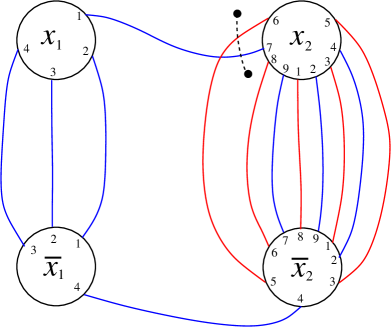
Figure 4.

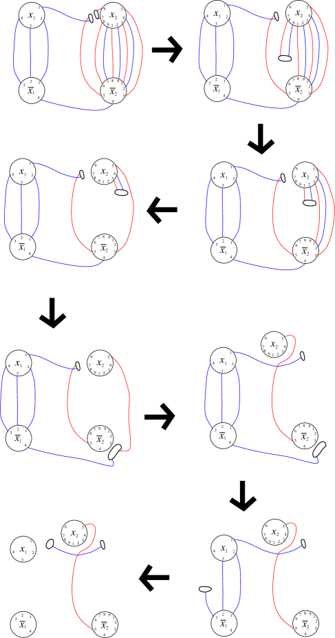
Figure 5.

In Case (2), by Corollary 2.8, the chosen arc is not part of a one-handled circular decomposition. Again, we have to restart the program choosing a different arc to drill out.

2.6.3. Some definitions

Now let $\gamma$ and $\gamma^{\prime}$ be two $\partial$–parallel properly embedded arcs in $E(F)$ disjoint with $\Gamma$, with $\partial$–parallelism disks $z$ and $z^{\prime}$, respectively; let $\{x_{1},\dots,x_{g}\}$ be a meridional system of disks for $E(F)$, and let $G$ be the corresponding Whitehead graph with respect to this system of disks. Then, by an isotopy of $E(F)$, we may assume that $z$ and $z^{\prime}$ are contained in $E(x_{1}\cup\cdots\cup x_{g})$ and (the images of) $\gamma$ and $\gamma^{\prime}$ are disjoint with $G$.

Assume that for two faces of $G$, that is, two connected components $A,B\subset\partial E(x_{1}\cup\cdots\cup x_{g})-G$, the face $A$ contains an endpoint of $\gamma$ and one of $\gamma^{\prime}$, and the face $B$ contains the other two endpoints of $\gamma$ and $\gamma^{\prime}$. Then there is an isotopy of $E(x_{1}\cup\cdots\cup x_{g})$ that fixes point-wise $G$ and sends $\gamma$ onto $\gamma^{\prime}$. Such an isotopy exists for, being $\gamma$ and $\gamma^{\prime}$ $\partial$–parallel, they are unknotted properly embedded arcs in the 3–ball $E(x_{1}\cup\cdots\cup x_{g})$, and the isotopy can be chosen to fix $G$, for the endpoints of the arcs are, by pairs, in components of $\partial E(x_{1}\cup\dots\cup x_{g})-G$. Then we see that a class of ‘equivalent’ 2–handles in the Whitehead diagram of $(E(F),\Gamma)$ with respect to $x_{1},\dots,x_{g}$ is determined by pairs of faces of $G$ in $\partial E(x_{1}\cup\cdots\cup x_{g})$ (and conversely). That is, for $\partial$–parallel properly embedded arcs $\gamma,\gamma^{\prime}\subset E(x_{1}\cup\cdots\cup x_{g})$, the triples $(E(x_{1}\cup\cdots\cup x_{g}),G,\gamma)$ and $(E(x_{1}\cup\cdots\cup x_{g}),G,\gamma^{\prime})$ are homeomorphic if and only if $\gamma$ and $\gamma^{\prime}$ connect the same pair of faces of $G$.

This is a very useful fact. To search for a one-handled decomposition, one must only test a finite number of $\partial$–parallel arcs in some Whitehead diagram, and analyze as above: there are as many $\partial$–parallel arcs to check as pairs of faces of the corresponding Whitehead graph.

We end this section with some definitions. Assume the arc $\gamma$ is boundary parallel into $\partial E(F)$. Let $z$ be a $\partial$–parallelism disk for $\gamma$ such that $\partial z=\gamma\cup\gamma^{B}_{z}$, where $\gamma^{B}_{z}$ is an arc in $\partial E(F)$. Then, after a small isotopy of $z$, if necessary, $\gamma^{B}_{z}$ intersects the edges of $\Gamma$ transversely in a finite number of points. If $e_{1},\dots,e_{n}$ are the edges of $\Gamma$ that intersect $\gamma^{B}_{z}$ and each $e_{i}$ intersects only once with $\gamma^{B}_{z}$, we say that $\gamma$ encircles the edges $e_{1},\dots,e_{n}$. If $\gamma$ encircles the edges $e_{1},\dots,e_{n}$, and all $e_{i}$ are incident in the vertex $\xi$ of $\Gamma$, we say that the arc $\gamma$ is around the vertex $\xi$. Notice that if $e_{1},\dots,e_{n},e_{n+1},\dots,e_{n+m}$ are all the edges incident in the vertex $\xi$ of $\Gamma$, and $\gamma$ is around vertex $\xi$ encircling the edges $e_{1},\dots,e_{n}$, then $\gamma$ also encircles the edges $e_{n+1},\dots,e_{n+m}$. The length of $\gamma$ in $\Gamma$ is the minimal number of intersection points of $\gamma^{B}_{z}$ and $\Gamma$ among all $\partial$–parallelism disks $z$ for $\gamma$.

3. Primitive elements in spines

Let $\mathcal{F}$ be a free group. An element $x\in\mathcal{F}$ is called primitive if $x$ is part of some basis of $\mathcal{F}$. A set of elements $x_{1},x_{2},\dots,x_{k}\in\mathcal{F}$ are called associated primitive elements if they are contained in some basis of $\mathcal{F}$.

Let $H$ be a genus $g$ handlebody. A simple closed curve $\alpha\subset H$ represents a primitive element in $\pi_{1}(H)$ if and only if there is an essential properly embedded disk $D\subset H$ such that $\alpha\cap D$ consists of a single point. A set of simple closed curves $\alpha_{1},\dots,\alpha_{k}\subset H$ represent a set of associated primitive elements in $\pi_{1}(H)$ if and only if there is a system of meridional disks $D_{1},D_{2},\dots,D_{g}\subset H$ such that, up to renumbering, $\alpha_{i}\cap D_{i}$ consists of a single point, and $\alpha_{i}\cap D_{j}=\emptyset$ for $i\neq j$, $i=1,\dots,k$, and $j=1,\dots,g$.

Theorem 3.1.

Let $k\subset S^{3}$ be a knot, and let $F\subset E(k)$ be a free Seifert surface for $k$. Assume $E(F)$ is a handlebody of genus $g$.

If there exists a graph $\Gamma=a_{1}\vee\cdots\vee a_{g}$ such that $\Gamma$ is a spine for $F$ on $\partial E(F)$, and the $\ell$ curves $a_{1},\dots,a_{\ell}$ represent associated primitive elements of $\pi_{1}(E(F))$, then the handle number $h(F)\leq g-\ell$.

Proof.

We follow the plan in Remark 2.2 (2): we will exhibit a system of properly embedded arcs (the arcs $\beta_{j}^{I}$, below) which are the co-cores of $g-\ell$ 2–handles to be drilled out of $E(F)$, and a system of $g-\ell$ 2–disks ($D_{\ell+1},\dots,D_{g}$, below) which define the co-cores of $g-\ell$ 1–handles to be drilled out of $E(F\cup\bigcup_{j}\beta_{j}^{I})$

Let $D_{1},D_{2},\dots,D_{g}\subset E(F)$ be a system of meridional disks for $E(F)$ such that $|a_{i}\cap D_{i}|=1$, and $a_{i}\cap D_{j}=\emptyset$ for $i\neq j$, $i=1,\dots,\ell$, and $j=1,\dots,g$. This system of meridional disks exists, since $a_{1},\dots,a_{\ell}$ represent associated primitive elements of $\pi_{1}(E(F))$.

Let $P\subset E(F)$ be a regular neighbourhood of the base point $x_{0}\in\partial E(F)$ ($x_{0}$ is also the base point of the graph $\Gamma$). We visualize $P$ as a $2g$–gonal prism. See Figure 6. For $i=1,\dots,g$, let $T_{i}$ be a regular neighbourhood of $a_{i}$ in $E(F)$ such that $T_{i}\cap T_{j}=P$ if $i\neq j$. Write $\widehat{T}_{i}=\overline{T_{i}-P}$; then $\widehat{T}_{i}$ is a 3–ball. The intersection, $\widehat{T}_{i}\cap P=d_{i}^{+}\cup d_{i}^{-}$, is the disjoint union of two 2–disks $d_{i}^{+}$ and $d_{i}^{-}$ (see Figure 6). Also write $\partial d_{i}^{+}=\beta_{i}^{B}\cup\beta_{i}^{I}$ where $\beta_{i}^{B}$ is an arc in $\partial E(F)$, and $\beta_{i}^{I}$ is a properly embedded arc in $E(F)$. Finally, write $A_{i}=\overline{\partial T_{i}-(d_{i}^{+}\cup d_{i}^{-}\cup\partial E(F))}$ which is a 2–disk.

The arcs $\beta^{I}_{\ell+1},\dots,\beta^{I}_{g}$ are the co-cores of 2–handles in $E(F)$ to be drilled out, according to the plan in Remark 2.2 (2):

Notice that the exterior of each $\beta_{i}^{I}$, $E(\beta_{i}^{I})=\overline{E(F)-\mathcal{N}(\beta_{i}^{I})}\cong\overline{E(F)-\mathcal{N}(A_{i})}$, and this homeomorphism is the identity map outside a small neighbourhood of $A_{i}$.

Consider $V=\overline{E(F)-(\widehat{T}_{\ell+1}\cup\widehat{T}_{\ell+2}\cup\cdots\cup\widehat{T}_{g})}$. Then $V$ is a genus $g$ handlebody and $E(F)$ is a regular neighbourhood of $V$. We see that

$$\overline{E(F)-\cup_{\ell+1}^{g}\mathcal{N}(\beta_{i}^{I})}\cong\overline{E(F)-\cup_{\ell+1}^{g}\mathcal{N}(A_{i})}\cong V\cup(g-\ell\text{ 1--handles })$$

where the $g-\ell$ 1–handles are the $g-\ell$ balls $\widehat{T}_{i}$ attached along the disks $d_{i}^{+}$, $d_{i}^{-}$, $i=\ell+1,\dots,g$.

By the choice of the disks $\{D_{i}\}$, we see that $\overline{V-\cup_{\ell+1}^{g}\mathcal{N}(D_{i}\cap V)}$ is a regular neighbourhood of $a_{1}\vee\cdots\vee a_{\ell}$. Then $\overline{E(F)-(\cup_{\ell+1}^{g}\mathcal{N}(\beta_{i}^{I})+\cup_{\ell+1}^{g}\mathcal{N}(D_{i}\cap V))}$ is a regular neighbourhood of $\Gamma$. In other words, $\mathcal{N}(F)\cup\{\mathcal{N}(\beta_{i}^{I})|i=\ell+1,\dots,g\}\cup\{\mathcal{N}(D_{i}\cap V)|i=\ell+1,\dots,g\}$ determines a circular handle decomposition of $E(k)$ based on $F$, as in Remark 2.2 (2). Therefore, $h(F)\leq g-\ell$.

∎

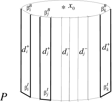
Figure 6. The neighbourhood of $x_{0}$.

Corollary 3.2 (The case “$\ell=g$”).

Let $k\subset S^{3}$ be a knot, and let $F$ be a free Seifert surface for $k$. Assume $E(F)$ is a handlebody of genus $g$.

If there exists a graph $\Gamma=a_{1}\vee a_{2}\vee\cdots\vee a_{g}$ such that $\Gamma$ is a spine for $F$ on $\partial E(F)$, and the curves $a_{1},\dots,a_{g}$ form a basis of $\pi_{1}(E(F))$, then $k$ is a fibered knot with fiber $F$.

Proof.

In this case $h(F)=0$, therefore, $E(F)$ admits a product structure $E(F)=F\times I$ induced by $\Gamma$, and $k$ is fibered with fiber $F$. ∎

Corollary 3.3 (The case “$\ell=0$”).

Let $k\subset S^{3}$ be a knot, and let $F\subset E(k)$ be a free Seifert surface for $k$. Assume $E(F)$ is a handlebody of genus $g$.

Then $h(k)\leq g$.

Proof.

By Theorem 3.1, considering $\ell=0$, we have $h(F)\leq g$. Therefore, $h(k)\leq g$. ∎

Remark 3.4.

Corollary 3.3 asserts that for a connected knot $k$, $h(k)\leq 2g_{f}(k)$. See [6] for another proof of this fact (a fact called the ‘Free Genus Estimate’ in [6]).

Corollary 3.5.

If $k$ is a connected free genus one knot, then $h(k)=0,1$, or $2$.

$\Box$

Remark 3.6.

Let $k$ be a connected free genus one knot in $S^{3}$ such that $k$ is not fibered (that is, $k\neq 3_{1},4_{1}$). At this point we can give some estimates for $cw(k)$:

If $k$ is almost fibered, it follows from Corollary 3.5 that $cw(k)=4$, or $cw(k)=6$. In any case, that is, if $k$ is almost fibered or not, $cw(k)\leq 6$.

If $k$ is not almost fibered, consider a circular decomposition $E(k)=(F\times I)\cup B_{1}\cup P_{1}\cup B_{2}\cup P_{2}\cup\cdots\cup B_{n}\cup P_{n}$, $n>1$, and $B_{i},P_{i}\neq\emptyset$, which realizes $cw(k)$. Then there are Seifert surfaces for $k$, $T_{1},\dots,T_{n}=F,S_{1},\dots,S_{n}\subset E(k)$, such that $S_{i}$ is obtained from $T_{i-1}$ by adding the 1-handles $B_{i}$, and $T_{i}$ is obtained from $S_{i}$ by adding the 2-handles $P_{i}$, and $cw(k)=(c(S_{\sigma(1)}),\dots,c(S_{\sigma(n)}))$ with $c(S_{\sigma(1)})\geq\cdots\geq c(S_{\sigma(n)})$ where $c(S)=1-\chi(S)$.

Now all $T_{i}$ are incompressible (Remark 2.3), and of genus one. For, if some $T_{j}$ is of genus at least two, then $S_{j}$ is of genus at least three, and the complexity $c(S_{j})\geq 6$. But then, since $n>1$, $cw(k)=(c(S_{\sigma(1)}),\dots,c(S_{\sigma(n)}))>6$, a contradiction. It follows that $cw(k)=(4,\dots,4)$.

That is, if $k$ is a connected non-fibered free genus one knot, then $cw(k)=4,6$, or $(4,\dots,4)$.

As it was mentioned in the Introduction, a connected non-fibered free genus one knot in $S^{3}$ is almost fibered (Theorem 6.7 below). It follows that $cw(k)\in\{4,6\}$.

Example 3.7.

Rational knots. If $k\subset S^{3}$ is a non-fibered rational knot, then $h(k)=1$. Also $cw(k)=4g(k)$ if $k$ is connected, and $cw(k)=4g(k)+1$ otherwise.

Let $k\subset S^{3}$ be a rational knot. Then $k$ is encoded with a continued fraction of the form $[2b_{1},2b_{2},\dots,2b_{g}]$ where $g$ is even or odd if $k$ is connected or not, respectively. Here $b_{1},\dots,b_{g}$ are non-zero integers . Now $k$ has a minimal genus Seifert surface $F$ as in Figure 7 (see [1], Answer 1.19). This surface is free. Note that $g(F)=g/2$ if $k$ is connected, and $g(F)=(g-1)/2$ otherwise.

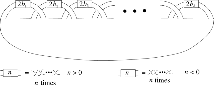
Figure 7. A minimal genus Seifert surface for the knot $k=[2b_{1},2b_{2},\dots,2b_{n}]$.

In a neighbourhood $V$ of this surface we can find a spine $\Gamma\subset F\times\{0\}\subset\partial V$ with $\Gamma=a_{1}\vee a_{2}\vee\cdots\vee a_{g}$, as in Figure 8.

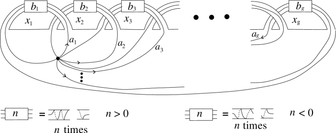
Figure 8. A spine for $k=[2b_{1},2b_{2},\dots,2b_{g}]$ in $\partial\mathcal{N}(F)$.

For the obvious meridional disks, $x_{1},x_{2},\dots,x_{g}$, of the handlebody $E(F)$, corresponding to a basis $\{x_{1},x_{2},\dots,x_{g}\}$ of $\pi_{1}(E(F))$, the curves $a_{1},a_{2},\dots,a_{g}$ represent the elements $x_{1}^{b_{1}}$, $x_{2}^{b_{2}}x_{1}$, $x_{3}^{b_{3}}x_{2}\dots$, $x_{g-1}^{b_{g-1}}x_{g-2}$, $x_{g}^{b_{g}}x_{g-1}$ of $\pi_{1}(E(F))$, respectively.

If each $|b_{i}|=1$, then $a_{1},a_{2},\dots,a_{g}$ represent a basis of $\pi_{1}(E(F))$, and, by Corollary 3.2, $k$ is fibered with fiber $F$.

If some $|b_{i}|\geq 2$, then $\{x_{g},x_{2}^{b_{2}}x_{1},x_{3}^{b_{3}}x_{2}\dots,x_{g-1}^{b_{g-1}}x_{g-2},x_{g}^{b_{g}}x_{g-1}\}$ is a basis for $\pi_{1}(E(F))$; it follows that the curves $a_{2},a_{3},\dots,a_{g}\subset\Gamma$ represent associated primitive elements of $\pi_{1}(E(F))$, and, by Theorem 3.1, $h(k)\leq h(F)=1$. By the second part of the statement of Answer 1.19 of [1], $k$ is not fibered. Therefore, $0<h(k)=h(F)=1$, and $cw(k)=2g$ if $k$ is connected, and $cw(k)=2g+1$ otherwise.

Remark 3.8.

In Theorem 3.21 of [3] it is claimed that the result in Example 3.7, the one-handledness of rational knots, is known, but unpublished.

Example 3.9.

Pretzel knots. The pretzel knot $k=P(\pm 3,q,r)$ with $|q|,|r|$ odd integers $\geq 3$, has $h(k)=1$ and, therefore, $cw(k)=4$.

Let $k$ be the pretzel knot $P(p,q,r)$ with $p,q,r$ odd integers. Then $k$ is a connected knot, and the ‘black surface’ $F$ of a standard projection of $k$ is a free genus one Seifert surface for $k$. See Figure 9.

Figure 9. Black surface for $P(7,9,9)$.

If $|p|,|q|,|r|\geq 3$, it is known that (1) $k$ has a unique incompressible Seifert surface (see [4]), namely, the free black surface $F$ of genus one; (2) $k$ has tunnel number two (see [7]); (3) $h(k)\leq 2$ (see Corollary 3.5); (4) since $t(k)\neq 1$, $k$ is not a rational knot; (5)  also $k$ is not fibered (that is, $k\neq 3_{1},4_{1}$).

For any permutation $s,t,u$ of $p,q,r$, the pair $(S^{3},k)$ is homeomorphic to a pair $(S^{3},\ell)$ where $\ell$ is a pretzel knot $P(s,t,u)$. Also, by a reflection, $P(p,q,r)$ is equivalent to $P(-p,-q,-r)$. Then, by Remark 2.1, we may assume that it holds either, Case 1: “$p,q,r>0$”, or Case 2: “$p<0$ and $q,r>0$”.

There is a spine shown in Figure 9 for the surface $F\times\{0\}\subset\partial\mathcal{N}(F)$. This spine is a $\theta$–graph. To obtain a wedge of circles as a spine $\Gamma=a_{1}\vee a_{2}\subset F\times\{0\}\subset\partial\mathcal{N}(F)$, we slide the middle edge of the $\theta$–graph to the left. In Case 1, “$p,q,r>0$”, we obtain the upper part of Figure 10; and, in Case 2, “$p<0$ and $q,r>0$”, after using an isotopy to avoid unnecessary intersections of the curve $a_{2}$ with the disk $x_{1}$, we obtain the lower part of Figure 10.

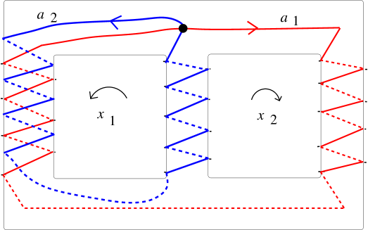
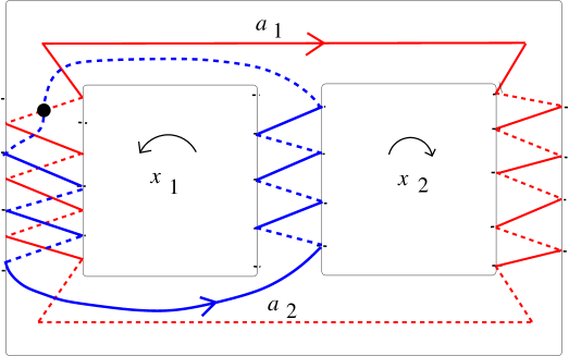
Figure 10. Spines for $P(p,q,r)$.

We see that, writing $\pi_{1}(E(F))\cong\langle x_{1},x_{2}:-\rangle$:

Case 1, ($p,q,r>0$), the curves $a_{1}$ and $a_{2}$ represent the elements $x_{2}^{(r+1)/2}x_{1}^{-(p-1)/2}$ and $x_{1}^{(p+1)/2}(x_{2}x_{1})^{(q-1)/2}$, respectively, in $\pi_{1}(E(F))$, or,

Case 2, ($p<0$ and $q,r>0$), the curves $a_{1}$ and $a_{2}$ represent the elements $x_{2}^{(r+1)/2}x_{1}^{(|p|+1)/2}$ and $x_{1}^{-(|p|-3)/2}(x_{2}x_{1})^{(q-3)/2}x_{2}$, respectively, in $\pi_{1}(E(F))$.

Assume the number $3\in\{|p|,q,r\}$.

In Case 1, “$p,q,r>0$”, using a homeomorphism of $S^{3}$, we may assume $p=3$. In this case the curve $a_{1}\simeq x_{2}^{(r+1)/2}x_{1}^{-1}$ represents a primitive element of $\pi_{1}(E(F))$ for, the set $\{x_{2}^{(r+1)/2}x_{1}^{-1},x_{2}\}$ is a basis of $\pi_{1}(E(F))$. Therefore, by Theorem 3.1, $h(k)=h(F)=1$, and $cw(k)=4$.

In Case 2, “$p<0$ and $q,r>0$”, if $p=-3$, then the curve $a_{2}\simeq(x_{2}x_{1})^{(q-3)/2}x_{2}$ represents a primitive element of $\pi_{1}(E(F))$ for, the set $\{(x_{2}x_{1})^{(q-3)/2}x_{2},x_{2}x_{1}\}$ is a basis of $\pi_{1}(E(F))$. If $q=3$ or $r=3$, we may assume that $q=3$, and then the curve $a_{2}\simeq x_{1}^{(|p|-3)/2}x_{2}$ represents a primitive element of $\pi_{1}(E(F))$ for, the set $\{x_{1}^{-(|p|-3)/2}x_{2},x_{1}\}$ is a basis of $\pi_{1}(E(F))$.

In both cases, $p=-3$, or $q$ or $r=3$, we conclude by Theorem 3.1, $h(k)=h(F)=1$, and $cw(k)=4$.

Remark 3.10.

If $|q|,|r|$ are odd integers $\geq 3$, then $k=P(\pm 3,q,r)$ has tunnel number two. Then the family of pretzel knots $\{P(\pm 3,q,r):|q|,|r|\text{ odd integers }\geq 3\}$ is a family of examples of non-fibered knots $k$ for which the strict inequality $h(k)<t(k)$ holds (compare with [10], where it is proved that $h(k)\leq t(k)$).

4. Pretzel knots: the case $|p|,|q|,|r|\geq 5$

In this section we show:

Theorem 4.1.

The free genus one Seifert surface for a pretzel knot $P(p,q,r)$ with $|p|,|q|,|r|\geq 5$ has handle number two.

As noted in Example 3.9, when dealing with the pretzel knot $k=P(p,q,r)$ we may assume: Case 1: “$p,q,r>0$”, or Case 2: “$p<0$ and $q,r>0$”.

4.1. Handle decompositions of $E(P(p,q,r))$

Lemma 4.2.

Let $V$ be a handlebody and let $\alpha\subset V$ be a properly embedded arc. If the exterior $E(\alpha)\subset V$ is a handlebody, then $\alpha$ is parallel into $\partial V$.

Proof.

By hypothesis, $\pi_{1}(E(\alpha))$ is a finitely generated free group. If $\mathcal{N}(\alpha)=D^{2}\times I$ is a regular neighbourhood of $\alpha$ in $V$, let $\mu=\partial D^{2}\times\{1/2\}$ be a meridian of $\mathcal{N}(\alpha)$. If $N\langle\mu\rangle$ denotes the normal closure of the element represented by $\mu$ in $\pi_{1}(E(\alpha))$, then $\pi_{1}(E(\alpha))/N\langle\mu\rangle$ is isomorphic to the fundamental group of the space obtained from $E(\alpha)$ by adding a 2–handle along $\mu$. Then $\pi_{1}(E(\alpha))/N\langle\mu\rangle\cong\pi_{1}(V)$ is a free group. It follows that $\mu$ represents a primitive element in $\pi_{1}(E(\alpha))$ (see [17], Theorem 4). Thus, there is an essential disk $\delta\subset E(\alpha)$ such that the number of points $\#(\delta\cap\mu)=1$. After an isotopy, we may assume that $\partial\delta\cap\partial N(\alpha)=\gamma$ is an arc, and $\partial\delta=\beta\cup\gamma$ where $\beta$ is an arc contained in $\partial V$.

There is a product 2–disk $Z=(\textrm{radius of }D^{2})\times I$ between $\gamma$ and $\alpha$, with $Z\subset\mathcal{N}(\alpha)$ for some product structure $D^{2}\times I$ of $\mathcal{N}(\alpha)$. Then $\delta$ can be extended to a disk $\delta^{\prime}=Z\cup\delta$ whose boundary is a union of arcs $\alpha\cup\beta^{\prime}$ with $\beta^{\prime}\subset\partial V$ (and $\beta\subset\beta^{\prime}$). Therefore, $\alpha$ is parallel into $\partial V$. ∎

Corollary 4.3.

Let $F$ be a free Seifert surface for a knot $k$. Suppose $F$ has handle number one and let $\alpha$ be the core of the 1–handle of a one-handled circular decomposition of $E(k)$ based on $F$. Then $\alpha$ is parallel into $\partial E(F)$.

Proof.

As in Remark 2.2 (2), the one-handled decomposition of the pair $(E(F),F)$ is constructed by, first, drilling a 2–handle out of $E(F)$ disjoint with, say, $F\times\{1\}$. This 2–handle has as co-core the arc $\alpha$ of the statement (cf. Remark 2.6.1). After drilling out $\alpha$, we, secondly, drill one 1–handle $B$ out of the exterior $E(\alpha)\subset E(F)$ with $B$ disjoint with $F\times\{1\}$. The result of this drilling is a regular neighbourhood of the surface $F\times\{0\}$ in $E(k)$ which is a handlebody. Therefore, the exterior $E(\alpha)$ in $E(F)$ is the union of the neighbourhood of $F\times\{0\}$ and the 1–handle $B$; that is, $E(\alpha)$ is a handlebody. By Lemma 4.2 we conclude that $\alpha$ is parallel into $\partial E(F)$.

∎

Proof of Theorem 4.1.

Let $F$ be the free genus one Seifert surface for $k=P(p,q,r)$ with $|p|,|q|,|r|$ odd integers $\geq 5$.

For the sake of contradiction, we assume that $F$ has handle number one. By Corollary 4.3, the core $\gamma$ of the 1–handle of the circular decomposition of $E(k)$ based on $F$ is parallel into $\partial E(F)$. By assumption, there is also a 2–handle $B\cong I\times D^{2}$ that completes the decomposition, such that the exterior $E(\gamma\cup B)\subset E(\gamma)$ is a regular neighbourhood of $F$ in $E(k)$, and $\partial B$ is disjoint with $F$. In particular the core, $\{1/2\}\times D^{2}$, of $B$ is an essential disk in $E(\gamma)$ disjoint with $F$.

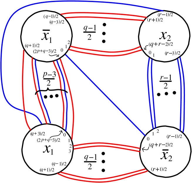
Figure 11.

We will show that any essential disk in $E(\gamma)$ intersects $F$, obtaining the desired contradiction.

Case 1: “$p,q,r>0$”. Let $\Gamma=a_{1}\vee a_{2}$ be the spine for $F$ given in Example 3.9. By Remark 2.5, we only need to analyze the handle decompositions of $(E(F),\Gamma)$. There is an obvious system of meridional disks $x_{1},x_{2}\subset E(F)$ as depicted in the upper part of Figure 10. The Whitehead diagram for $(E(F),\Gamma)$ with respect to $x_{1},x_{2}$ looks like Figure 11.

In the corresponding Whitehead graph $G$ we see:

• Four fat vertices corresponding to the meridional disks $x_{1}$ and $x_{2}$.

• There are $(q-1)/2$ horizontal edges connecting $\bar{x}_{1}$ and $x_{2}$, and $(q-1)/2$ horizontal edges connecting $x_{1}$ and $\bar{x}_{2}$; all these horizontal arcs belong to the curve $a_{2}$.

• There are $(r-1)/2$ vertical edges connecting $x_{2}$ and $\bar{x}_{2}$; one diagonal edge connecting $x_{1}$ and $x_{2}$, and one diagonal edge connecting $\bar{x}_{1}$ and $\bar{x}_{2}$; all these vertical and diagonal edges belong to the curve $a_{1}$.

• Finally, connecting $x_{1}$ with $\bar{x}_{1}$, we find, going from right to left in Figure 11, first an arc belonging to $a_{2}$, and then we find $(p-3)/2$ pairs of arcs belonging consecutively to $a_{1}$ and $a_{2}$; and a last arc belonging to $a_{2}$ which crosses with the diagonal arc from $x_{1}$ to $x_{2}$ on the base point of $\Gamma$.

Claim 0: Let $z$ be a $\partial$–parallelism disk for the arc $\gamma$ in $E(F)$. Then the disk $z$ contains at least one point of $a_{1}$ and one point of $a_{2}$.

Proof.

Let $G_{i}$ be the Whitehead graph of the pair $(E(F),a_{i})$ with respect to $x_{1},x_{2}$ ($i=1,2$). See Figure 12. After sliding the handle defined by the disk $x_{2}$ along the handle defined by $\bar{x}_{1}$ on the right side of Figure 12, the image of the graph $G_{2}$ looks like Figure 13. Since these graphs are connected and contain no cut vertex, it follows from Corollary 2.8 that any essential disk in $E(F)$ intersects $a_{i}$ ($i=1,2$). Now, the exterior $E(\gamma)$ can be regarded as a copy of $E(F)$ plus one 1–handle defined by the disk $z$. Assume $z\cap a_{2}\neq\emptyset$. If $z\cap a_{1}=\emptyset$, then $a_{1}$ is contained in the copy of $E(F)\subset E(\gamma)$. By hypothesis there is an essential disk $\Delta\subset E(\gamma)$ such that $\Delta\cap(a_{1}\cup a_{2})=\emptyset$. Now, $\Delta\cap z\neq\emptyset$, otherwise $\Delta$ is a subset of the copy of $E(F)\subset E(\gamma)$ missing the extra 1–handle, and $\Delta\cap a_{1}=\emptyset$, contradicting that any essential disk in $E(F)$ intersects $a_{1}$. Through isotopies, we may assume that $\Delta\cap z$ is a set of disjoint arcs. Then the intersection of $\Delta$ with the copy of $E(F)\subset E(\gamma)$, that is, the set $\Delta\cap\overline{(E(\gamma)-\mathcal{N}(z))}$, is a set of disjoint properly embedded disks $\Delta_{1},\dots,\Delta_{n}\subset E(F)$. Since $\Delta$ is not parallel to $z$ in $E(\gamma)$, at least one $\Delta_{i}$ is essential in $E(F)$, otherwise $\Delta$ would be parallel into $\partial E(\gamma)$. We obtain again an essential disk in $E(F)$ disjoint with $a_{1}$, which is a contradiction as above, and, therefore, $z\cap a_{1}\neq\emptyset$. ∎

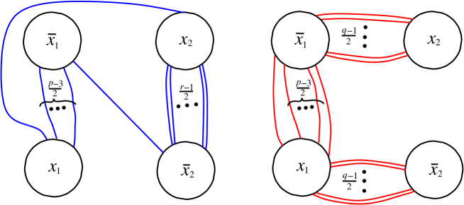
Figure 12. The graphs of curves $a_{1}$ and $a_{2}$

The arc $\gamma$, being $\partial$–parallel in $E(F)$ by Corollary 4.3, can be isotoped into this Whitehead diagram as a properly embedded arc with ends disjoint with $G$ (that is, after an isotopy of $E(F)$, we may assume that $\gamma$ is disjoint with the system of disks $x_{1}$ and $x_{2}$). Recall that we are assuming that $\gamma$ is the core of a 1–handle of a one-handled circular decomposition of $E(k)$ based on $F$. Therefore, after drilling out $\gamma$, there is an essential disk in $E(\gamma)$ disjoint with $\Gamma$; that is, after drilling out $\gamma$, and obtaining a new Whitehead diagram with six fat vertices with Whitehead graph $G^{\prime}$, there is a sequence of handle slides of $E(\gamma)$ that disconnect the graph $G^{\prime}$, giving an essential disk in $E(F)$ disjoint with $\Gamma$ (see Section 2.6).

Let $G_{i}$ be the Whitehead graph of the pair $(E(F),a_{i})$ with respect to $x_{1},x_{2}$. See Figure 12. After drilling out the arc $\gamma$ from the diagram of $G_{i}$, we obtain a new Whitehead diagram for $(E(\gamma),a_{i})$ with six fat vertices, corresponding to $x_{1},x_{2}$, and $z$, and with Whitehead graph $G_{i}^{\prime}$. Performing the handle slides of $E(\gamma)$ as above, the image of the graph $G_{i}^{\prime}$ will be also disconnected, giving an essential disk in $E(\gamma)$ disjoint with $a_{i}$ ($i=1,2$).

Notice that if we drill out an arc of length one in $G_{i}$ and perform handle slides, the image of $G_{i}$ is disconnected (it contains four isolated fat vertices), $i=1,2$. We deal with this kind of arcs after Claims 1 and 2.

Claim 1: Let $\alpha$ be a properly embedded arc in $(E(F),a_{2})$, disjoint with $a_{2}$, such that $\alpha$ is parallel into $\partial E(F)$, and $\alpha$ has length at least two in $G_{2}$. Then any essential disk in $E(\alpha)$ intersects $a_{2}$.

Proof.

The arc $\alpha$ minimally encircles a number of edges of the graph $G_{2}$. For example, the arc that encircles the two diagonal edges in Figure 13 actually has length 0.

Now, after sliding the handle defined by the disk $x_{2}$ along the handle defined by $\bar{x}_{1}$ on the right side of Figure 12, the image of the graph $G_{2}$ looks like Figure 13. The fat vertices of this graph are also obtained from the images of the disks $x_{1}$ and $x_{2}$ after the slide. We still call this new graph and new disks $G_{2}$, and $x_{1}$, $x_{2}$, respectively. This graph has $(q-3)/2$ vertical edges connecting $x_{2}$ with $\bar{x}_{2}$, one diagonal edge connecting $x_{2}$ with $\bar{x}_{1}$, one diagonal edge connecting $x_{1}$ with $\bar{x}_{2}$, and there are $(p-1)/2$ vertical arcs connecting $x_{1}$ with $\bar{x}_{1}$.

Let $z$ be a minimal $\partial$–parallelism disk for $\alpha$ in $E(F)$, and let $G$ be the Whitehead graph of $(E(\alpha),a_{2})$ with respect to $x_{1},x_{2}$, and $z$, which is obtained from $G_{2}$, by cutting along $z$ and adding two fat vertices $z$ and $\bar{z}$.

Case “Length of $\alpha=2$”: Since $p\geq 5$, there are at least two vertical edges connecting $x_{1}$ and $\bar{x}_{1}$. Then there are two types of arcs of length two for the edges of $G_{2}$ around $x_{1}$ as in Figure 13, for, any arc encircling two consecutive edges of $G_{2}$ connecting $x_{1}$ and $\bar{x}_{1}$ can be slid in $E(F)$ into an arc of type 1 or type 2. See Figure 14 where the arcs that can be slid in $E(F)$ into an arc of type 2 are shown.

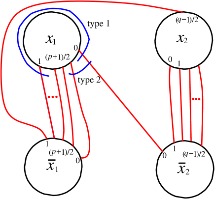
Figure 13.

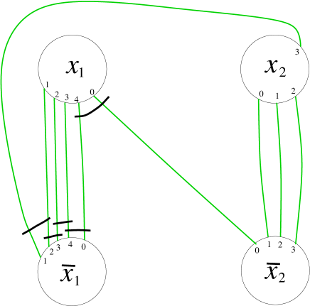
Figure 14.

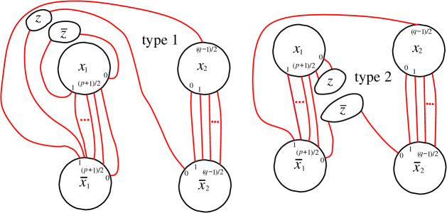
Figure 15.

After drilling out the arc $\alpha$, if $\alpha$ is of type 1, or of type 2, the new Whitehead graph contains a cut vertex (see Figure 15).

After sliding handles, as in Section 2.6, we end up with a graph $G_{2}^{\prime}$ with its simple associated graph a cycle of six vertices and six edges; that is, this simple graph contains no cut vertex. Therefore, $G^{\prime}_{2}$ contains no cut vertex, and by Corollary 2.8, $a_{2}$ intersects every essential disk of $E(\alpha)$.

If $q\geq 7$, there are at least two vertical edges connecting $x_{2}$ and $\bar{x}_{2}$. Then, by symmetry, the analysis of arcs of length two around $x_{2}$ and $\bar{x}_{2}$ is the same as for arcs of length two around $x_{1}$ and $\bar{x}_{1}$.

If $q=5$, there is a single vertical edge connecting $x_{2}$ and $\bar{x}_{2}$, and, then, there are no arcs of length two around $x_{2}$ or $\bar{x}_{2}$.

For arcs not around a vertex of $G_{2}$, there are two more types of arcs of length two as in Figure 16,

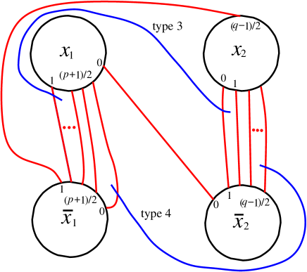
Figure 16.

but, after drilling out the arc $\alpha$ of type 3 or 4, the new Whitehead graph contains no cut vertex, and then, by Corollary 2.8, $a_{2}$ intersects every essential disk of $E(\alpha)$.

Case “Length of $\alpha\geq 3$”: If $\alpha$ is an arc around $x_{i}$, we may assume that the length of $\alpha$ in $G_{2}$ is between 3 and $degree(x_{i})/2$ (see last paragraph of Section 2.6.1), and $\alpha$ contains a sub-arc of type 1 or 2. After drilling out the arc $\alpha$ and sliding, if there appear cut vertices, we end up with a graph with its simple associated graph a cycle with six vertices and six edges. Therefore, $a_{2}$ again intersects every essential disk of $E(\alpha)$.

If $\alpha$ is of length at least 3, and $\alpha$ contains a sub-arc of type 3 or 4, then, after drilling out the arc $\alpha$, the new Whitehead graph contains no cut vertex, and, by Corollary 2.8, we conclude that $a_{2}$ intersects every essential disk of $E(\alpha)$.

By the final remarks of Section 2.6.1, the arcs of type 1-4 exhaust all arcs to be considered as arcs of a one-handled decomposition for $G_{2}$.

∎

Claim 2: Let $\alpha$ be a properly embedded arc in $(E(F),a_{1})$, disjoint with $a_{1}$, such that $\alpha$ is parallel into $\partial E(F)$, and $\alpha$ has length at least two in $G_{1}$. Then any essential disk in $E(\alpha)$ intersects $a_{1}$.

Proof.

The Whitehead graph $G_{1}$ of $(E(F),a_{1})$ has a shape as in Figure 13, but with $(r-1)/2$ vertical edges connecting $x_{2}$ with $\bar{x}_{2}$, one diagonal edge connecting $x_{2}$ with $\bar{x}_{1}$, one diagonal edge connecting $x_{1}$ with $\bar{x}_{2}$, and there are $(p-3)/2$ vertical arcs connecting $x_{1}$ with $\bar{x}_{1}$.

A similar (symmetric) analysis as in Claim 1, gives that $a_{1}$ intersects every essential disk of $E(\alpha)$.

∎

We are assuming that, after drilling out the arc $\gamma$, there is a set of handle slides of $E(\gamma)$ that disconnect the graph $G^{\prime}$, giving an essential disk in $E(F)$ disjoint with $\Gamma$.

By Claims 1 and 2, $\gamma$ is of length one in $G_{1}$, and of length one in $G_{2}$. If $\gamma$ is around one fat vertex $\xi$ of $G$, it might happen that $\gamma$ encircles exactly one edge of $G_{1}$, and all but one edge of $G_{2}$, or vice versa. In this case, $\gamma$ is around either $x_{2}$ or $\bar{x}_{2}$. There are four arcs around $x_{2}$, and four arcs around $\bar{x}_{2}$ of this kind. The four arcs with this property around $\bar{x}_{2}$ can be slid in $E(F)$ and become equivalent to the four arcs around $x_{2}$ in Figure 17; see Section 2.6.1.

Figure 17.

After drilling out $\gamma$, there is a cut vertex in the new Whitehead graph, and a single handle slide produces a graph $G^{\prime}$ with no cut vertices. By Corollary 2.8, there are no essential disks disjoint with $G$ in $E(\gamma)$. Another possibility is that $\gamma$ encircles all but one edge of $G_{1}$ and all but one edge of $G_{2}$, but in this case, $\gamma$ also encircles exactly one edge of $G_{1}$, and exactly one edge of $G_{2}$.

There are four types of arcs of length two encircling exactly one edge of $G_{1}$ and exactly one edge of $G_{2}$ (see Figure 18). Again, any arc encircling two edges of $G$, one of $G_{1}$ and one of $G_{2}$ can be slid in $E(F)$ into an arc of type 1, type 2, type 3, or type 4; see Section 2.6.1.

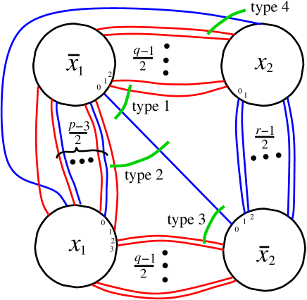
Figure 18.

After drilling out the arc $\gamma$, if $\gamma$ is of type 1, type 2, type 3, or type 4, the new Whitehead graph contains a cut vertex. After sliding, we end up with a graph $G^{\prime}$ with its simple associated graph as one of the drawings in Figure 19. Since these graphs contain no cut vertex, by Corollary 2.8,

Figure 19.

we conclude that any essential disk in $E(\gamma)$ intersects $G$, and, therefore, intersects $\Gamma\subset F$. This contradiction shows that $h(F)\neq 1$. Since $k=P(p,q,r)$ is not fibered, and $h(F)\leq 2$, by Corollary 3.5, it follows that $h(F)=2$, when $p,q,r\geq 5$.

This finishes Case 1.

Case 2: “$p<0$, and $q,r>0$”. As in Example 3.9, we construct a spine $\Gamma=a_{1}\vee a_{2}$ for $F$ starting with the spine shown in Figure 9, but now we slide the middle edge of the $\theta$–graph rightwards. The spine $\Gamma$ looks like Figure 20, and the Whitehead diagram for $(E(F),\Gamma)$ with respect to the system of disks $x_{1},x_{2}$ is as in Figure 21. By Remark 2.5, we only need to analyze the handle decompositions of $(E(F),\Gamma)$.

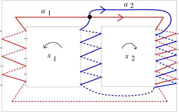
Figure 20.

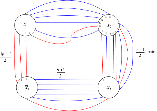
Figure 21.

The Whitehead graphs $G_{1}$ and $G_{2}$ of the pairs $(E(F),a_{1})$ and $(E(F),a_{2})$, respectively, are shown in Figure 22. Although these diagrams are similar to the diagrams in Figure 12 of Case 1, the configuration of the diagram for $a_{1}$ here is not the same as the configuration of the positive case (Case 1); that is, the corresponding Whitehead diagrams are not isomorphic.

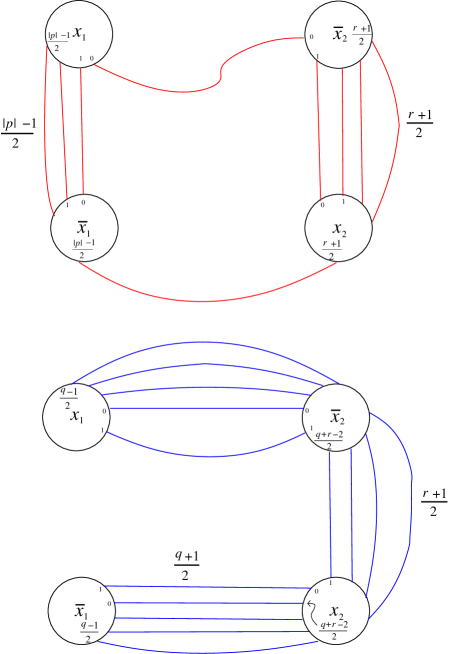
Figure 22.

However, the analysis of the different properly embedded arcs in the Whitehead diagrams of $(E(F),a_{1})$, $(E(F),a_{2})$, and $(E(F),\Gamma)$, giving rise to a possible one-handled decomposition, is completely similar as in Case 1.

The Whitehead diagram for $(E(F),a_{2})$ is isomorphic to the corresponding Whitehead diagram of Case 1. Then

Claim 1: Let $\alpha$ be a properly embedded arc in $(E(F),a_{2})$, disjoint with $a_{2}$, such that $\alpha$ is parallel into $\partial E(F)$, and $\alpha$ has length at least two in $G_{2}$. Then any essential disk in $E(\alpha)$ intersects $a_{2}$.
$\Box$

Claim 2: Let $\alpha$ be a properly embedded arc in $(E(F),a_{1})$, disjoint with $a_{1}$, such that $\alpha$ is parallel into $\partial E(F)$, and $\alpha$ has length at least two in $G_{1}$. Then any essential disk in $E(\alpha)$ intersects $a_{1}$.

Proof.

We first analyze arcs of length 2 in $G_{1}$. The arcs around vertices $x_{1}$ and $\bar{x}_{1}$ are shown in Figure 23. There are only two types after sliding the arcs in $E(F)$.

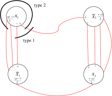
Figure 23.

After drilling out the arc $\alpha$, if $\alpha$ is of type 1, or of type 2, the new Whitehead graph contains a cut vertex, but after sliding handles, as in Section 2.6.1, we end up with a graph $G_{1}^{\prime}$ with its simple associated graph a cycle of six vertices and six edges; that is, this simple graph contains no cut vertex. Therefore, $G^{\prime}_{1}$ contains no cut vertex, and by Corollary 2.8, $a_{2}$ intersects every essential disk of $E(\alpha)$.

For arcs of length 2 around the vertices $x_{2}$ and $\bar{x}_{2}$, the analysis is identical to Case 1.

For arcs not around a vertex of $G_{1}$, there are two more types of arcs of length two as in Figure 24,

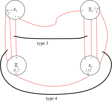
Figure 24.

but, after drilling out the arc $\alpha$ of type 3 or 4, the new Whitehead graph contains no cut vertex, and then, by Corollary 2.8, $a_{2}$ intersects every essential disk of $E(\alpha)$.

For arcs of length at least three, we follow the same argument as in Case 1, and conclude that $a_{2}$ intersects every essential disk of $E(\alpha)$.

∎

Recall that we are assuming that $\gamma$ is the core of a 1–handle of a one-handled circular decomposition of $E(k)$ based on $F$. In view of Claims 1 and 2, as in Case 1, we see that the arc $\gamma$ encircles exactly one edge of $G_{1}$, and exactly one edge of $G_{2}$.

There are four types of arcs of length two encircling exactly one edge of $G_{1}$ and exactly one edge of $G_{2}$ (see Figure 25). For, any arc encircling two edges of $G$, one of $G_{1}$ and one of $G_{2}$ can be slid in $E(F)$ into an arc of type 1, type 2, type 3, or type 4 (Section 2.6.1).

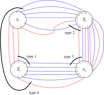
Figure 25.

After drilling out the arc $\gamma$, if $\gamma$ is of type 1, type 2, type 3, or type 4, the new Whitehead graph contains a cut vertex. After sliding, we end up with a graph $G^{\prime}$ with its simple associated graph as one of the drawings in Figure 26. Since these graphs contain no cut vertex, by Corollary 2.8,

Figure 26.

we conclude that any essential disk in $E(\gamma)$ intersects $G$, and, therefore, intersects $\Gamma\subset F$. Thus, $h(F)\neq 1$. Since $k=P(p,q,r)$ is not fibered, and $h(F)\leq 2$, by Corollary 3.5, it follows that $h(F)=2$, when $p\leq-5$ and $q,r\geq 5$.

This finishes Case 2, and also the proof of Theorem 4.1.

∎

Corollary 4.4.

Let $k$ be the pretzel knot $P(p,q,r)$ with $|p|,|q|,|r|\geq 5$. Then $cw(k)=6$.

Proof.

Since $k$ has a unique incompressible Seifert surface, by Remark 2.3 it follows that $cw(k)\in\mathbb{Z}$. By Theorem 4.1, $cw(k)=6$. ∎

Remark 4.5.

Theorem 4.1 gives a family of knots of genus one and handle number two. This answers in the affirmative a question in [6]: Does there exist a knot $k$ with $h(k)>g(k)$?

5. Genus one essential surfaces and powers of primitive elements

In this section we show that if $k$ is a free genus one knot with at least two non-isotopic Seifert surfaces, then the free Seifert surface of $k$ admits a special type of spine. This result is essential to prove the main theorem of Section 6 (Theorem 6.7).

Lemma 5.1.

Let $H$ be a handlebody of genus $g\geq 2$, and let $\alpha\subset\partial H$ be a simple closed curve. Assume that there is a primitive element $p\in\pi_{1}(H)$ such that $\alpha$ represents an element conjugate with $p^{n}$ for some $n\in\mathbb{Z}$, $n\neq 0$. Then there is an essential 2–disk $D\subset H$ such that $D\cap\alpha=\emptyset$.

Proof.

Consider a basis $\{p,q_{2},\dots,q_{g}\}$ for $\pi_{1}(H)$. Then $\pi_{1}(H)=\langle p\rangle*\langle q_{2},\dots,q_{g}\rangle$ is a non-trivial splitting, and $\alpha$ is conjugate with $p^{n}\in\langle p\rangle$. Then $\{\alpha\}$ is separable in $\pi_{1}(H)$, and the disk $D$ is obtained by Theorem 3.2 of [15]. ∎

Let $\Gamma\cong a_{1}\vee a_{2}$ be a graph in the boundary of a genus two handlebody $H$. We say that $a_{2}$ spoils disks for $a_{1}$ if for any essential disk $D\subset H$ such that $D\cap a_{1}=\emptyset$, the number of points $\#(D\cap a_{2})\geq 2$.

Theorem 5.2.

Let $k\subset S^{3}$ be a non-trivial connected knot, and let $F\subset E(k)$ be a free genus one Seifert surface for $k$.

There is another genus one Seifert surface for $k$ which is not equivalent to $F$ if and only if there exists a spine $\Gamma=a_{1}\vee a_{2}$ for $F$ in $\partial\mathcal{N}(F)$ such that $a_{1}$ represents an element conjugate to $g^{n}$ with $n\geq 2$ for some primitive element $g\in\pi_{1}(E(F))$, and $a_{2}$ spoils disks for $a_{1}$.

Proof.

Let $\Gamma=a_{1}\vee a_{2}$ be a spine for $F$ such that $a_{1}$ represents an element conjugate to $g^{n}$ with $n\geq 2$ for some primitive element $g\in\pi_{1}(E(F))$, and $a_{2}$ spoils disks for $a_{1}$

Let $D\subset E(F)$ be an essential properly embedded disk such that $a_{1}\cap D=\emptyset$, which is given by Lemma 5.1. We may assume that $H_{1}=\overline{E(F)-\mathcal{N}(D)}$ is a solid torus. Let $A_{1}$ be a regular neighbourhood of $a_{1}$ in $\partial E(F)$; then $A_{1}\subset\partial H_{1}$. Write $B_{1}=\overline{\partial H_{1}-A_{1}}$. Since $|n|\geq 2$, the annuli $A_{1}$ and $B_{1}$ are non-parallel in $H_{1}$. We push $Int(B_{1})$ into $H_{1}$ to obtain $B_{1}^{\prime}$, a properly embedded annulus in $H_{1}$.

Let $\mathcal{N}(a_{2})\subset\partial E(F)$ be a regular neighbourhood of $a_{2}$ such that $A_{1}\cap\mathcal{N}(a_{2})$ is a rectangle; then $B_{2}=\overline{\mathcal{N}(a_{2})-A_{1}}$ is a ‘band’ (that is, a 2–disk) such that $B_{2}\cap A_{1}=B_{2}\cap B_{1}^{\prime}$ is a pair of arcs in $\partial B_{1}^{\prime}$. Then $G=B_{2}\cup B_{1}^{\prime}$ is a genus one Seifert surface for $k$ (we push $Int(G)$ slightly into $E(F)$ to get a properly embedded surface in $E(F)$).

Now, $\widehat{G}=G\cap H_{1}$ is the union of the annulus $B_{1}^{\prime}$ with the disk components of $\widehat{B}_{2}=B_{2}\cap H_{1}$. Notice that $\partial\widehat{B}_{2}\subset B_{1}\subset\partial H_{1}$.

By hypothesis $\#(a_{2}\cap D)\geq 2$; thus, $\widehat{G}$ is disconnected, and the components of $\widehat{G}$ are $B_{1}^{\prime}\cup(\text{two 2--disks of }\widehat{B}_{2})$, and at least one sub-disk $z\subset\widehat{B}_{2}$ with $\partial z\subset Int(B_{1})$.

Since $|n|\geq 2$, we cannot push $B_{1}^{\prime}$ onto $A_{1}$ in $H_{1}$. Then a $\partial$–parallelism for $\widehat{G}$ in $H_{1}$ contains a $\partial$–parallelism $W$ for $B_{1}^{\prime}$ onto $B_{1}$, but then $W$ contains the 2–disk $z\subset\widehat{G}$. Therefore, $\widehat{G}$ is not parallel into $\partial H_{1}$. We conclude that $G$ is not boundary parallel in $E(F)$ for, a $\partial$–parallelism for $G$ induces a $\partial$–parallelism for $\widehat{G}$. It follows that $G$ and $F$ are not equivalent. This finishes sufficiency.

Now, if there is another genus one Seifert surface for $k$ which is not equivalent to $F$, we can find still another non-equivalent genus one Seifert surface $G\subset E(k)$ for $k$ such that $G$ and $F$ have disjoint interiors; see [13]. We write $k=G\cap\partial E(F)$.

The surface $G$ splits $E(F)$ into two handlebodies, $H_{0}\cup H_{1}=\overline{E(F)-\mathcal{N}(G)}$, of genus two for $H_{0}$ and $H_{1}$ are irreducible and, since $G$ is $\pi_{1}$–injective into $H_{0}$ and $H_{1}$, it follows that $H_{0}$ and $H_{1}$ are $\pi_{1}$–injective into $E(F)$; therefore, $H_{0}$ and $H_{1}$ have free fundamental groups. We assume $\partial H_{i}=G\cup(F\times\{i\})$ plus a neighbourhood of $k$, $i=0,1$. By considering a system of disks for the handlebody $E(F)$, we see that there is a disk $D\subset E(F)$ that $\partial$–compresses $G$ in $E(F)$, and $D$ is contained in, say $H_{0}$, and is properly embedded in $H_{0}$.

Then $k$ is a $((1,0),(n,m))$–curve in $\partial H_{0}$ (Lemma 4.3 of [16]) with $|k\cap D|=2$. See Figure 27.

Figure 27. Surfaces $G$ and $F\times\{0\}$ in $H_{0}$.

Cutting $H_{0}$ along $D$ we obtain a solid torus $V\subset H_{0}$ such that $\widehat{G}=G\cap V$ is an $(n,m)$–torus annulus in $\partial V$; and the complementary annulus $\widehat{F}=\overline{\partial V-\widehat{G}}$ contains, and is isotopic, to $(F\times\{0\})\cap V$ in $\partial V$ with an isotopy fixed outside a regular neighbourhood of $D$.

Let $a_{1}\subset F\times\{0\}$ be the core of the annulus $\widehat{F}$, and let $b_{1}\subset\widehat{G}$ be the core of the annulus $\widehat{G}$.

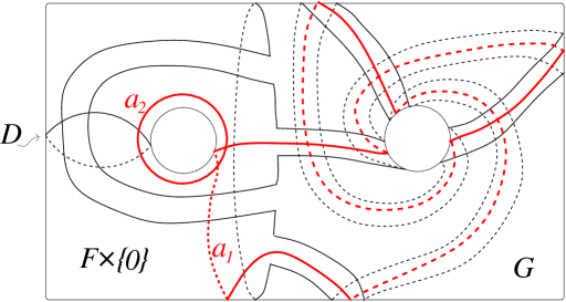
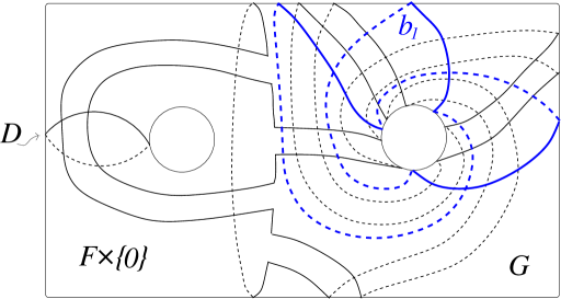
Figure 28. $\Gamma=a_{1}\vee a_{2}$ and $b_{1}$.

Let $C^{\prime}\subset\partial V$ be a 2–disk that contains the pair of disks $\partial V\cap\mathcal{N}(D)$, and let $C\subset H_{0}$ be a properly embedded disk with $\partial C=\partial C^{\prime}$. Now let $Z\subset H_{0}$ be a meridional disk such that $Z\cap C=\emptyset$. Then $\widetilde{F}=(F\times\{0\})\cap(\overline{H_{0}-\mathcal{N}(Z)})$ contains a (1,0)–annulus $A$ in the solid torus $\overline{H_{0}-\mathcal{N}(Z)}$. Let $a_{2}\subset Int(F\times\{0\})$ be the core of $A$, where we can arrange that $a_{1}\cap a_{2}$ is just one point. Then $\Gamma=a_{1}\vee a_{2}$ is a spine for $F$. See Figure 28.

The curve $a_{2}$ spoils disks for $a_{1}$ in $E(F)$ for, otherwise, there is an essential disk $D\subset E(F)$ such that $D\cap a_{1}=\emptyset$, and the number of points $\#(D\cap a_{2})<2$. If $D\cap a_{2}=\emptyset$, since $\Gamma$ is a spine for $F$, the surface $F$ is contained in the solid torus $E(D)\subset E(F)$; it follows that $F$ is compressible in $E(D)$, and, thus, $F$ is compressible in $E(F)$. But, since $k$ is non-trivial, and $g(F)=1$, $F$ is incompressible in $E(k)$. Then $D\cap a_{2}$ is just one point, and $D\cap\partial F$ is a set of two points. We may assume that $D$ intersects $k=\partial G$ in exactly two points. Since $G$ is incompressible, we may arrange that $D\cap G$ is just one arc. Now, this arc is essential in $G$ for, otherwise, we can slide $G$ along $D$, and obtain $G^{\prime}$ homotopic to $G$ in $E(F)$ such that $G^{\prime}$ is contained in the solid torus $E(D)$; then $G^{\prime}$ is not $\pi_{1}$–injective, and, since $G$ and $G^{\prime}$ are homotopic embeddings, thus, $G$ is not $\pi_{1}$–injective; but that makes $G$ compressible. Then $\widehat{G}=G\cap E(D)$ is an annulus, therefore, $\widehat{G}$ is parallel into $\partial E(D)$. Using the disk $D$ we can extend this parallelism to a parallelism of $G$ into $\partial E(F)$, contradicting that $G$ is essential in $(E(F),k)$.

Now, $a_{1}\subset F\times\{0\}$ represents, up to conjugacy, the same element as $b_{1}\subset G$ in $\pi_{1}(H_{0})$ for, they are disjoint curves on a torus, and therefore, parallel.

Observe that, since $G$ is not parallel to $F\times\{0\}$, we have $|n|\geq 2$. In particular $\widehat{G}$ and $\widehat{F}$ are not parallel in $V$.

We now explore $H_{1}$.

Recall $D$ is a $\partial$–compression disk for $G$ in $E(F)$; in particular $D\cap\partial E(F)$ is an arc. It follows that, to recover $E(F)$ from $\overline{E(F)-\mathcal{N}(D)}$, we attach to $\overline{E(F)-\mathcal{N}(D)}$ the 3–ball $\mathcal{N}(D)$ along a disk. Then $\overline{E(F)-\mathcal{N}(D)}$ is a genus 2 handlebody. In fact $E(F)$ is a regular neighbourhood of $\overline{E(F)-\mathcal{N}(D)}$. In particular, the inclusion induces an isomorphism $\pi_{1}(\overline{E(F)-\mathcal{N}(D)})\rightarrow\pi_{1}(E(F))$.

Since $\overline{E(F)-\mathcal{N}(D)}=H_{1}\cup_{\widehat{G}}V$, then $H_{1}\cup_{\widehat{G}}V$ is a genus two handlebody. Therefore, the core $b_{1}$ of $\widehat{G}$ represents a primitive element $\beta_{1}\in\pi_{1}(H_{1})$ for, if $\pi_{1}(V)=\langle v;-\rangle$, then $b_{1}$ represents $v^{n}$, which is not primitive in $V$. The element $\beta_{1}$ is part of a basis, say, $\pi_{1}(H_{1})=\langle w,\beta_{1}:-\rangle$. By Seifert-van Kampen, $\pi_{1}(E(F))\cong\pi_{1}(H_{1}\cup_{\widehat{G}}V)=\langle w,\beta_{1},v:\beta_{1}=v^{n}\rangle\cong\langle w,v:-\rangle$. That is, $v$ is primitive in $\pi_{1}(E(F))$, and $b_{1}$ represents $v^{n}$.

∎

6. Free genus one knots are almost fibered

In this section we show that all free genus one knots are almost fibered. We give here an outline of the plan of the proof:

Start with a non-fibered free genus one knot $k$ with a genus one free Seifert surface $F\subset E(k)$. If $k$ has a unique Seifert surface, then $k$ is almost fibered (Remark 2.3). If $k$ were not almost fibered, then as in Remark 3.6, $k$ has a genus one Seifert surface not isotopic to $F$. By Theorem 5.2, there is a spine $\Gamma=a_{1}\vee a_{2}$ for $F$ in $\partial\mathcal{N}(F)$ such that $a_{1}$ represents an element conjugate to $g^{p}$ with $p\geq 2$ for some primitive element $g\in\pi_{1}(E(F))$, and $a_{2}$ spoils disks for $a_{1}$. By Lemma 5.1, we can find an essential disk $\Delta\subset E(F)$ with $\Delta\cap a_{1}=\emptyset$, and the exterior $E(\Delta)=\overline{E(F)-\mathcal{N}(\Delta)}$ is the disjoint union of two solid tori, $V_{0},V_{1}$ with, say, $a_{1}\subset\partial V_{0}$. We regard $\Delta\subset\partial V_{0}$. Then $\Gamma\cap V_{0}$ consists of the curve $a_{1}$, which is a $(p,q)$–curve in $V_{0}$, and an arc with endpoints on $\partial\Delta$ intersecting $a_{1}$ in exactly one point, and a set of parallel arcs with endpoints on $\partial\Delta$ which are disjoint with $a_{1}$. See Figure 32.

In Section 6.1 we show how to find a properly embedded arc in $V_{0}$ disjoint with $\Gamma$ which, in Section 6.2, is shown to be the core of the 1–handle of a one-handled circular decomposition for $E(k)$ based on $F$. In this analysis, the disk $\Delta$ is regarded as ‘unreachable’, and should be thought as very near the point at infinity. That is, all homeomorphisms in this subsection will fix point-wise the disk $\Delta$.

6.1. Handles for torus manifolds

Let $p$ and $q$ be a pair of coprime integers. Consider the points $\{s_{\ell}\}_{\ell=1}^{p}\subset S^{1}$ with $s_{\ell}=e^{2\pi i\ell/p}$; also let $\widetilde{V}$ be the cylinder $D^{2}\times I$, and write $s_{\ell}^{I}=s_{\ell}\times I\subset\widetilde{V}$. The rotation $\rho_{q}$ of angle $2\pi q/p$ on $D^{2}$ gives a quotient $P:(\widetilde{V},\cup_{\ell=1}^{p}s_{\ell}^{I})\rightarrow(V,\alpha)$, where $V$ is the solid torus obtained from $\widetilde{V}$ by identifying $(z,0)$ with $(\rho_{q}(z),1)$ for each $z\in D^{2}$, and $\alpha$ is the simple closed curve on $\partial V$ obtained as the image of the union $\cup_{\ell=1}^{p}s_{\ell}^{I}$ in this quotient. The rotation $\rho_{q}$ acts on $\{s_{\ell}\}_{\ell=1}^{p}$ as the cyclic permutation of order $p$ such that $\rho_{q}(s_{i})=s_{i+q}$ where subindices are taken $\mod p$. We consider also a fixed point $\infty\in\alpha$, the ‘point at infinity’. The homeomorphism type of the pair $(V,\alpha)$ is called the $(p,q)$–torus sutured manifold, or simply the $(p,q)$–manifold. Throughout this section we assume $0<q<p$. Notice that the $(p,q)$–torus sutured manifold $(V,\alpha)$ is not a sutured manifold, but $\alpha$ is a spine of a small regular neighbourhood $\mathcal{N}(\alpha)\subset\partial V$, and the pair $(V,\mathcal{N}(\alpha))$ is a true sutured manifold with suture $\alpha$.

In the following, we perform several operations on the $(p,q)$–manifold (drilling of arcs, homeomorphisms, etc.), and it will be done in such a way that the point at infinity of the manifold will remain fixed.

Let $x\subset V$ be the meridional disk $P(D^{2}\times\{0\})$. From the pair $(\widetilde{V},\cup_{\ell=1}^{p}s_{\ell}^{I})$ we give a Whitehead diagram for the $(p,q)$–manifold $(V,\alpha)$ associated to $x$ as follows:

We regard $\tilde{V}=D^{2}\times I$ as the exterior $E(x)\subset V$, and write $x$ and $\bar{x}$ for $D^{2}\times\{0\}$ and $D^{2}\times\{1\}$, respectively. The arcs $s_{1}^{I},\dots,s_{p}^{I}$ are the edges of $G$, the corresponding Whitehead graph with fat vertices $x$ and $\bar{x}$. To obtain a Whitehead diagram, we have to number the endpoints of $s_{1}^{I},\dots,s_{p}^{I}$. In a plane projection of the graph $G$, we assume that the unbounded face of $G$ contains the edges $s_{q}^{I}$ and $s_{q+1}^{I}$. See Figure 29. The point at infinity is either the middle point of $s_{q}^{I}$, or the middle point of $s_{q+1}^{I}$. If $\infty\in s_{q}^{I}$, then we rename $v_{j}=(s_{j},0)$ and $\bar{v}_{j}=(\rho_{q}(s_{j}),1)=(s_{j+q},1)$; if $\infty\in s_{q+1}^{I}$, we rename $v_{j}=(s_{j+q},0)$ and $\bar{v}_{j}=(\rho_{q}(s_{j+q}),1)=(s_{j+2q},1)$ where subindices are taken $\mod{p}$. In any case, we number the point $v_{i}$ with the number $i$, and the point $\bar{v}_{j}$ with the number $j$ ($i,j=1,\dots,p$). Also, we write $\alpha_{i}$ for the edge of $G$ such that $v_{i}\in\alpha_{i}$.

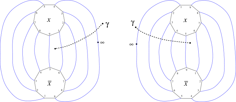
Figure 29. Whitehead diagrams for the (9,4)–manifold and the (9,5)–manifold

This diagram and the corresponding Whitehead graph are called the $(p,q)$–diagram and the $(p,q)$–graph, respectively. Notice that the edge $\alpha_{1}$ connecting $x$ with $\bar{x}$ starting at the point numbered $1\in x$ ends at the point numbered $p-q+1\in\bar{x}$.

Remark 6.1.

Consider a Whitehead diagram of a pair $(V,\alpha)$ associated to $x$ where $V$ is a solid torus, $\alpha$ is a simple closed curve on $\partial V$, and $x$ is a meridional disk of $V$. If in the fat vertices of the Whitehead diagram of $(V,\alpha)$, the points corresponding to ends of edges are numbered with elements of the set $\{1,\dots,p\}$ consecutively in the positive (negative) direction on $x$ (on $\bar{x}$), in a compatible way with the gluing homeomorphism to recover the $V$, then if the edge connecting $x$ with $\bar{x}$ starting at the point numbered $1\in x$ ends at the point numbered $t\in\bar{x}$, then $t=p-q+1$; that is, the Whitehead diagram corresponds to the $(p,q)$–torus sutured manifold with $q=p-t+1$.

Let $(V,\alpha)$ be the $(p,q)$–torus sutured manifold, and let $G$ be the Whitehead graph of $(V,\alpha)$ with respect to a meridional disk $x\subset V$. Let $\gamma$ be a properly embedded arc in $V$, such that $\gamma$ is around the vertex $x$ in the Whitehead diagram of $(V,\alpha)$ with respect to $x$, and $\gamma$ encircles the edges $\alpha_{1},\dots,\alpha_{q}$. Also, assume that $\gamma$ lies ‘above’ the point $\infty\in\alpha$, that is, $\gamma$ is between $\infty$ and $x$. See Figure 29. The arc $\gamma$ is called the canonical 2–handle of length $q$ for the $(p,q)$–manifold. Note that the arc $\gamma$ is the co-core of a 2–handle in $V$.

If we drill out the canonical 2–handle of length $q$, we obtain a Whitehead diagram with respect to the system of disks $x,z\subset E(\gamma)\subset V$ where $z$ is the obvious $\partial$–parallelism disk for $\gamma$. See Figure 30.

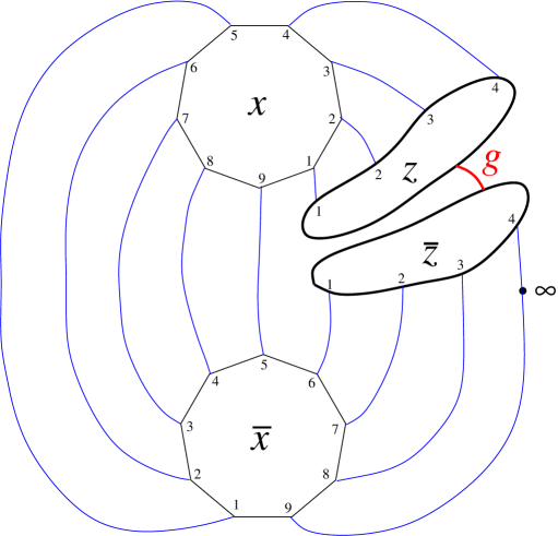
Figure 30.

We refer to this Whitehead diagram as the Whitehead diagram obtained by drilling out the canonical 2–handle of length $q$ of the $(p,q)$–manifold. Notice that the arc $g$ in Figure 30 is a ‘longitude’ for the handle defined by $z$. That is, if we glue back the disks $z$ and $\bar{z}$ and kill the longitude $g$ with a 2–handle, we recover the Whitehead diagram of the $(p,q)$–manifold. In practice, we just join the ends of the edges in $z$ with the ends of the edges in $\bar{z}$ with parallel arcs on the diagram, and delete the disks $z$ and $\bar{z}$ from the picture, and we get the Whitehead diagram of the $(p,q)$–manifold back.

Let $G$ be the graph of the Whitehead diagram obtained by drilling out the canonical 2–handle of length $q$ of the $(p,q)$–manifold. Then $G$ is a graph with four fat vertices $x,\bar{x},z$, and $\bar{z}$; there are $q$ edges connecting $z$ and $x$; there are $q$ edges connecting $\bar{z}$ and $\bar{x}$; and there are $p-q$ edges connecting $x$ with $\bar{x}$. Compare with Figure 30. Note that $x$ is a cut vertex of $G$ (and $z$ and $\bar{z}$ are not cut vertices); then we can slide the handle corresponding to $z$ along the handle defined by $x$

After sliding, if the new disk $x$ is still a cut vertex, we can again slide the new disk $z$ along the new disk $x$, and so on. Let $G^{\prime}$ be the image of the graph $G$ after $\kappa$ handle slides of $z$ along $x$. The graph $G^{\prime}$ is called the $\kappa$–slid graph obtained from the $(p,q)$–graph $G$.

Lemma 6.2.

Let $p,q$ be a pair of coprime integers, $0<q<p$, and assume that

$$p=\kappa_{1}q+r_{1},\textrm{ with }0\leq r_{1}<q,\textrm{ and }\kappa_{1}\geq 1$$

Let $G$ be the graph of the Whitehead diagram obtained by drilling out the canonical 2–handle of length $q$ of the $(p,q)$–manifold, and let $G^{\prime}$ be the $\kappa_{1}$–slid graph obtained from the $(p,q)$–graph $G$. Then $G^{\prime}$ is the graph of the Whitehead diagram obtained by drilling out the canonical 2–handle of length $r_{1}$ of the $(q,r_{1})$–manifold. The point at infinity is a fixed point of these handle slides.

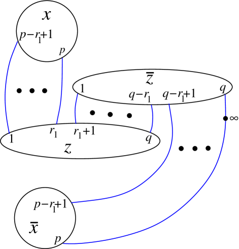
Figure 31. After sliding $z$ along $x$

Proof.

In the Whitehead graph $G$, the ends of the edges connecting the disk $z$ with the disk $x$, are numbered $1,2,\dots,q$ in the disk $x$; these ends are the points $v_{1},v_{2},\dots,v_{q}$ in $\partial x$. Then, after sliding $z$ along $x$, the new disk $z$ carries the edges with ends that were numbered $1,2,\dots,q$ in $\bar{x}$. Thus, now the ends of the edges connecting $z$ and $x$, after the slide, have ends which are the image of the rotation $\rho_{q}$ of angle $2\pi q/p$ of the points $v_{1},v_{2},\dots,v_{q}$; that is, the ends are the points $v_{q+1},v_{q+2},\dots,v_{2q}$ which are numbered $q+1,q+2,\dots,2q$ in $x$.

We see that after sliding $\kappa_{1}-1$ times $z$ along $x$, the ends of the edges connecting $z$ and $x$ are numbered $(\kappa_{1}-1)q+1,(\kappa_{1}-1)q+2,\dots,\kappa_{1}q$ in $x$. Then after sliding $\kappa_{1}$ times $z$ along $x$, the points still connected by edges in $x$ are numbered $\kappa_{1}q+1,\kappa_{1}q+2,\dots,p$. Now, by hypothesis $p=\kappa_{1}q+r_{1}$, then $\kappa_{1}q+1=p-r_{1}+1$, which means that there are $r_{1}$ points left in $x$. That is, see Figure 31, we have a graph, the image of $G$ after the slides, with fat vertices $x,\bar{x},z,\bar{z}$; there are $r_{1}$ edges connecting $x$ with $z$; there are $r_{1}$ edges connecting $\bar{x}$ with with $\bar{z}$; and there are $q-r_{1}$ edges connecting $z$ with $\bar{z}$. Now, the edge with one end in $z$ numbered with 1 has the other end numbered with $p-r_{1}+1\in x$; and the edge with one end in $\bar{x}$ numbered with $p-r_{1}+1$ has the other end in $\bar{z}$ numbered with $q-r_{1}+1$.

Therefore, the new diagram is the Whitehead diagram obtained by drilling out the canonical 2–handle of length $r_{1}$ of the $(q,r_{1})$–manifold. Since the disks $\bar{x}$, and $\bar{z}$ were never touched, the point at infinity is a fixed point of the handle slides.

Notice that if $q=1$, then $\kappa_{1}=p$, and $r_{1}=0$, and everything is easier: The image graph $G$ above, in this case, replacing the values of $q$ and $r_{1}$, has four fat vertices $x,\bar{x},z,\bar{z}$; there are $0$ edges connecting $x$ with $z$; there are $0$ edges connecting $\bar{x}$ with with $\bar{z}$; and there is $1$ edge connecting $z$ with $\bar{z}$. That is, after canceling the handle defined by $x$, we obtain the (1,0)–manifold. ∎

Corollary 6.3.

Let $r_{1},r_{2}$ be a pair of coprime integers, $0<r_{2}<r_{1}$. Assume

$$\begin{array}[]{lll}r_{1}=&\kappa_{1}r_{2}+r_{3},&0<r_{3}<r_{2}\\ r_{2}=&\kappa_{2}r_{3}+r_{4},&0<r_{4}<r_{3}\\ &\hfill\vdots\hfill&\hbox{}\hfill\vdots\hfill\\ r_{n-1}=&\kappa_{n-1}r_{n}+1,&0<1<r_{n}\\ r_{n}=&\kappa_{n},\end{array}$$

with $\kappa_{i}\geq 1$, $i=1,\dots,n$.

Let $G$ be the graph of the Whitehead diagram obtained by drilling out the canonical 2–handle of length $r_{2}$ of the $(r_{1},r_{2})$–manifold. Let $G_{1}$ be the $\kappa_{1}$–slid graph obtained from the $(r_{1},r_{2})$–graph $G$. For $i=1,\dots,n-1$, let $G_{i+1}$ be the $\kappa_{i+1}$–slid graph obtained from the $(r_{i},r_{i+1})$–graph $G_{i}$.

Then $G_{n}$ is the graph of the Whitehead diagram obtained by drilling out the canonical 2–handle of length $0$ of the $(1,0)$–manifold $(V,\alpha)$.

The point at infinity is a fixed point of these handle slides.

$\Box$

Remark 6.4.

The graph $G_{i}$ in the statement of Corollary 6.3 is the graph of the Whitehead diagram obtained by drilling out the canonical 2–handle of length $r_{i+2}$ of the $(r_{i+1},r_{i+2})$–manifold. Then $G_{i}$ is a graph with four fat vertices $\xi,\bar{\xi},\zeta$, and $\bar{\zeta}$. The symbols $\xi$ and $\zeta$ stand for the symbols $x$ and $z$ in some order (that is, the sets $\{\xi,\zeta\}$ and $\{x,z\}$ are equal, but just as unordered sets). There are $r_{i+2}$ edges connecting $\zeta$ and $\xi$; there are $r_{i+2}$ edges connecting $\bar{\zeta}$ and $\bar{\xi}$; and there are $r_{i+1}-r_{i+2}$ edges connecting $\xi$ with $\bar{\xi}$.

Remark 6.5.

Let $p,q$ be a pair of coprime integers, and assume that $p/q=[\kappa_{1},\dots,\kappa_{n}]$, as a continued fraction, with $\kappa_{i}\geq 1$ for each $i$.

1. Write $p_{i}/q_{i}=[\kappa_{1},\dots,\kappa_{i}]$ with $p_{i},q_{i}$ coprimes. Write $p_{0}=1,p_{-1}=0$, and $q_{0}=0,q_{-1}=1$. It is well known that $p_{i}=\kappa_{i}p_{i-1}+p_{i-2}$, and $q_{i}=\kappa_{i}q_{i-1}+q_{i-2}$; also $p_{i}q_{i-1}-p_{i-1}q_{i}=(-1)^{i}$ for $i\geq 1$. (Article 337 and 338 of [5]). Since $\kappa_{i}\geq 1$, one easily shows $p_{i}>q_{i}>0$ for $i\geq 1$. In particular, $p>q>0$. Note also that $p_{i+1}>p_{i}$.

2. Let $r,s$ be the two coprime integers $p_{n-1},q_{n-1}$, respectively, and let $(V,\alpha)$ be the $(p,q)$–manifold. Then the $(r,s)$–torus curve can be drawn on $\partial V$ as a simple closed curve, $\beta$, which intersects $\alpha$ exactly at the point at infinity for $ps-qr=\pm 1$. Note that if $n$ is even, then the point at infinity is at the right in the Whitehead diagram, and if $n$ is odd, it is at the left, as in Figure 29. The curve $\beta$ can be visualized on the Whitehead diagram of the $(p,q)$–manifold as a set of new edges connecting the fat vertices, and disjoint with the Whitehead graph, and a single new edge intersecting the Whitehead graph at the point at infinity. Conversely, the curve $\alpha$ can be visualized in a similar way on the Whitehead diagram of the $(r,s)$–manifold.

   Notice that between two edges of $\alpha$, there is at most one edge of $\beta$ for, $p>r$.

Theorem 6.6.

Assume $p/q=[\kappa_{1},\dots,\kappa_{n}]$ with $p,q$ coprime, and $\kappa_{i}\geq 1$ for each $i$. Let $r,s$ be the pair of coprime integers such that $r/s=[\kappa_{1},\dots,\kappa_{n-1}]$. Let $(V,\alpha)$ be the $(p,q)$–manifold, and let $\beta\subset\partial V$ be the $(r,s)$–torus curve such that $\alpha$ intersects $\beta$ exactly at the point at infinity.

If $\gamma\subset V$ is the canonical 2–handle of length $q$ of the $(p,q)$–manifold, then the exterior $E(\gamma)$ is a regular neighbourhood of $\alpha\cup\beta$.

Proof.

Let $G$ be the graph of the Whitehead diagram obtained by drilling out the canonical 2–handle of length $q$ of the $(p,q)$–manifold, but including the arcs of the curve $\beta$. Call $\alpha$–edges the edges of $G$ corresponding to the $(p,q)$–torus curve $\alpha$, and $\beta$–edges the edges of $G$ corresponding to the $(r,s)$–torus curve $\beta$.

Writing $r_{1}=p$, and $r_{2}=q$, the statement $p/q=[\kappa_{1},\dots,\kappa_{n}]$ with $\kappa_{i}\geq 1$ means: there are integers $r_{3},\dots,r_{n}$ such that

$$\begin{array}[]{lll}r_{1}=&\kappa_{1}r_{2}+r_{3},&0<r_{3}<r_{2}\\ r_{2}=&\kappa_{2}r_{3}+r_{4},&0<r_{4}<r_{3}\\ &\hfill\vdots\hfill&\hbox{}\hfill\vdots\hfill\\ r_{n-1}=&\kappa_{n-1}r_{n}+1,&0<1<r_{n}\\ r_{n}=&\kappa_{n}.\end{array}$$

See Remark 6.5, (1). Writing $\rho_{1}=r$ and $\rho_{2}=s$, the statement $r/s=[\kappa_{1},\dots,\kappa_{n-1}]$ means: there are integers $\rho_{3},\dots,\rho_{n-1}$ such that

$$\begin{array}[]{lll}\rho_{1}=&\kappa_{1}\rho_{2}+\rho_{3},&0<\rho_{3}<\rho_{2}\\ \rho_{2}=&\kappa_{2}\rho_{3}+\rho_{4},&0<\rho_{4}<\rho_{3}\\ &\hfill\vdots\hfill&\hbox{}\hfill\vdots\hfill\\ \rho_{n-2}=&\kappa_{n-2}\rho_{n-1}+1,&0<1<\rho_{n-1}\\ \rho_{n-1}=&\kappa_{n-1}.\end{array}$$

Notice that the canonical 2–handle of length $q$ for the $(p,q)$–manifold is the canonical 2–handle of length $q$ for the $\alpha$–edges of $G$, but it is also the canonical 2–handle of length $s$ for the $\beta$–edges of $G$. Then the graph $G_{n-1}$ of Corollary 6.3 (Remark 6.4) contains four fat vertices $\xi,\bar{\xi},\zeta$, and $\bar{\zeta}$. Note $r_{n+1}=1$; then there is a single $\alpha$–edge connecting $\zeta$ and $\xi$; there is a single $\alpha$–edge connecting $\bar{\zeta}$ and $\bar{\xi}$; and there are $r_{n}-1$ $\alpha$-edges connecting $\xi$ with $\bar{\xi}$. Note that $\rho_{n}=1$ and $\rho_{n+1}=0$; then there is a single $\beta$–edge connecting $\xi$ with $\bar{\xi}$ intersecting the $\alpha$–edge connecting $\bar{\zeta}$ and $\bar{\xi}$ at the point at infinity; and there are no more $\beta$–edges. The graph $G_{n}$ is obtained by sliding $\zeta$ through $\xi$ the number $\kappa_{n}=r_{n}$ of times. Then $G_{n}$ has a single $\alpha$–edge connecting $\xi$ with $\bar{\xi}$ and a single $\beta$–edge connecting $\zeta$ with $\bar{\zeta}$ intersecting at the point at infinity. The theorem follows.

Notice that when $q=1$, $n=1$, the graph $G_{n-1}=G$.

∎

6.2. One-handledness of knots

Theorem 6.7.

If $k$ is a non-fibered free genus one knot in $S^{3}$, then $k$ is almost fibered.

Proof.

Let $k\subset S^{3}$ be a knot, and let $F\subset E(k)$ be a genus one free Seifert surface for $k$. Assume $k$ is not almost fibered. Then, as in Remark 3.6, $k$ has another genus one Seifert surface disjoint and not equivalent to $F$. By Theorem 5.2 there is a spine $\Gamma=a_{1}\vee a_{2}$ for $F$ in $\partial\mathcal{N}(F)$ such that $a_{1}$ represents an element conjugate to $g^{p}$ with $p\geq 2$, for some primitive element $g\in\pi_{1}(E(F))$, and $a_{2}$ spoils the disks of $a_{1}$. We shall show that the existence of such graph $\Gamma$ implies $h(F)=1$, and, since $F$ is of minimal genus, therefore, $cw(k)=4$. This contradiction gives the theorem.

By Corollary 5.1, there is an essential 2–disk $\Delta\subset E(F)$ such that $\Delta\cap a_{1}=\emptyset$. We may assume that the exterior $E(\Delta)\subset E(F)$ is not connected, and is the union of two solid tori $H_{0}$ and $H_{1}$ with $a_{1}\subset H_{0}$. There is a copy of $\Delta$ in $\partial H_{0}$; then $a_{1}\subset\partial H_{0}-\Delta$. Write $T=\overline{\partial H_{0}-\Delta}$; $T$ is a once punctured torus. A properly embedded arc $\alpha\subset T$ is called a rel $\Delta$ curve in $\partial H_{0}$, and is visualized as the arc $\alpha$ union a properly embedded arc in $\Delta$ with the same ends as $\alpha$. Or rather, we may regard $\Delta$ as a point at infinity of the torus $T/\partial\Delta$.

We have that $a_{1}$ is a $(p,q)$–torus curve in $H_{0}$ for some $q$ (this implies that we have fixed a longitude-meridian pair in $\partial H_{0}$; by changing the longitude-meridian pair, we may assume that $0<q<p$). The intersection $a_{2}\cap H_{0}=a_{2}\cap\partial H_{0}$ is a set of disjoint arcs $c\cup b_{1}\cup\cdots\cup b_{m}\subset\partial H_{0}$ with ends in $\partial\Delta$ and such that $b_{i}\cap a_{1}=\emptyset$ for each $i$, and the set $c\cap a_{1}$ is a single point, the base point of $\Gamma$.

Regarding $c$ as a rel $\Delta$ curve, $c$ is an $(r,s)$–torus rel $\Delta$ curve in $H_{0}$ with $ps-qr=\pm 1$. Since $ps-qr=\pm 1$, any other pair $(r^{\prime},s^{\prime})$ such that $ps^{\prime}-qr^{\prime}=\pm 1$ is of the form $(r^{\prime},s^{\prime})=(r+\ell p,s+\ell q)$ for some integer $\ell$. Then by sliding $a_{2}$ along $a_{1}^{\pm 1}$ several times, we obtain a new spine for $F$. By Remark 2.5, we may assume that the arc $c$ is an $(r,s)$–torus rel $\Delta$ curve in $H_{0}$ where, if $p/q=[\kappa_{1},\dots,\kappa_{n}]$ as a continued fraction with terms $\kappa_{i}\geq 1$, then $r/s=[\kappa_{1},\dots,\kappa_{n-1}]$.

Since $b_{1},\dots,b_{m}\subset\partial H_{0}-(Int(\Delta)\cup a_{1}\cup c)\cong D^{2}$, then each of $b_{1},\dots,b_{m}$ are rel $\Delta$ curves parallel to $a_{1}$.

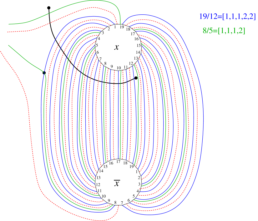
Figure 32. The (19,12) and (8,5)–torus curves

Now, consider the graph $G$ of the Whitehead diagram of the $(p,q)$–manifold $(H_{0},a_{1})$, and include in $G$ the edges induced by the rel $\partial$ curves $c,b_{1},\dots,b_{m}$. By deforming the diagram, we may assume that $\Delta$ is contained in a small neighbourhood of the point at infinity which is the base point of $\Gamma$, the point of intersection of $c$ and $a_{1}$. Let $\gamma$ be the canonical 2–handle of length $q$ for $(H_{0},a_{1})$. In the Whitehead diagram, we place $\gamma$ in such a way that it starts by encircling the arc $c$ coming from infinity, and then encircles the $q$ edges belonging to $a_{1}$ and whatever is in the middle, and nothing more (that is, after encircling the last edge belonging to $a_{1}$, the arc $\gamma$ does not encircle any arc belonging to $c$ or $b_{1},\dots,b_{m}$). See Figure 32 where the dotted line is a set of parallel arcs. We drill out $\gamma$ and, by Theorem 6.6, if we slide handles in the Whitehead diagram obtained by drilling $\gamma$ out of $H_{0}$, we obtain a sequence of diagrams as in Figures 33-38. All handle slides fix point-wise the small neighbourhood of the point at infinity, and, thus, also the disk $\Delta$.

The resulting Whitehead graph on $\partial H_{0}$ consists of four fat vertices $\xi,\bar{\xi},\zeta,\bar{\zeta}$; there is a single $a_{1}$–edge connecting $\xi$ and $\bar{\xi}$, and a single $c$–edge connecting $\zeta$ with $\bar{\zeta}$ intersecting in the base point of $\Gamma$ (In Figure 32, $\xi=z$ and $\zeta=x$). Notice that the $c$–arc is actually two arcs, one connecting $\zeta$ with $\partial\Delta$, and the other connecting $\partial\Delta$ with $\bar{\zeta}$. Without lost of generality, this last arc contains the base-point of $\Gamma$.

Let $v$ be a meridional disk for $H_{1}$ disjoint with $\Delta$. Then $\xi,\zeta$ and $v$ is a system of meridional disks for the handlebody $E(\gamma)$. Write $\pi_{1}(E(\gamma))=\langle\xi,\zeta,v:-\rangle$. Then $a_{1}$ represents the element $\xi$, and $a_{2}$ represents an element $\bar{\zeta}\cdot W(\xi,v)$ where $W(\xi,v)$ is a word in the letters $\xi$ and $v$. Since $\{\xi,\bar{\zeta}\cdot W(\xi,v),\zeta\}$ is a basis for $\pi_{1}(E(\gamma))$, it follows that $a_{1}$ and $a_{2}$ represent associated primitive elements. Then we can find a system of disks $D_{1},D_{2},D_{3}$ for $E(\gamma)$ such that $a_{i}\cap D_{i}$ is exactly one point, and $a_{i}\cap D_{j}=\emptyset$ for $i\neq j$, $i=1,2$, and $j=1,2,3$. Therefore, $\overline{E(\gamma)-\mathcal{N}(D_{3})}$ is a regular neighbourhood of $\Gamma=a_{1}\vee a_{2}$. We conclude that $D_{3}$ is the co-core of a 1–handle that, together with $\gamma$, gives a one-handled circular decomposition for $E(k)$ as in Remark 2.2 (2). Since $k$ is not fibered, it follows that $h(k)=1$, and that $k$ is almost fibered. This contradiction finishes the proof of the theorem.

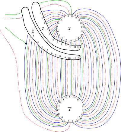
Figure 33. Slide $z$ along $x$

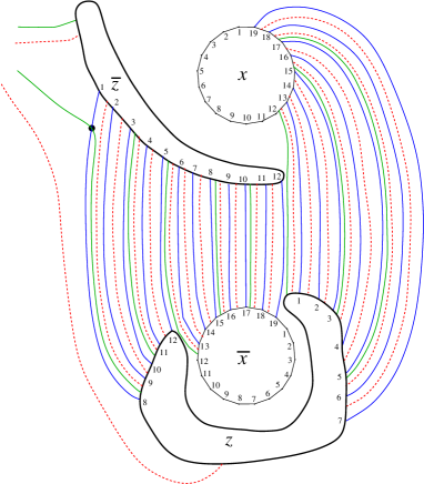
Figure 34. Slide $x$ along $z$

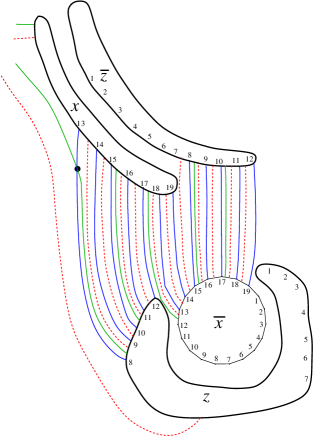
Figure 35. Slide $\bar{z}$ along $\bar{x}$

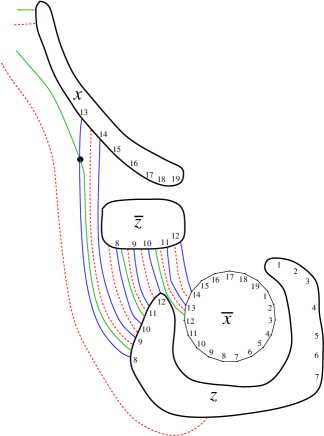
Figure 36. Slide twice $\bar{x}$ along $\bar{z}$

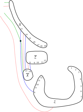
Figure 37. Slide twice $\bar{z}$ along $\bar{x}$

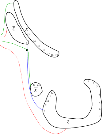
Figure 38. A long slide of $x$ deletes curve

∎

Remark 6.8.

By [10], a tunnel number one knot admits a one-handled circular decomposition based on some not specified surface. In [12] genus one knots with tunnel number one were classified, and it turns out that these knots are free genus one knots. Let $k$ be a non fibered genus one knot with tunnel number one. In Example 3.7, we considered the case that $k$ is simple, and in the proof of Theorem 6.7, we considered the case that $k$ is not simple. It follows that for these knots, their circular width is realized with a one-handled circular decomposition based on a minimal (genus one) free Seifert surface.

References

- [1] D. Gabai. Genera of the arborescent links. Memoirs of the Amer. Math. Soc. 339 (1986), 1–88.
- [2] H. Goda, On handle number of Seifert Surfaces in . Osaka J. Math., vol. 30 (1993), 63–80.
- [3] H. Goda. Circle valued Morse theory for knots and links. Clay Math. Proceedings 5 (2006), 71–99.
- [4] H. Goda, M. Ishiwata. A classification of Seifert surfaces for some pretzel links. Kobe J. Math. 23 (2006), 11–28.
- [5] H. S. Hall, S. R. Knight. Higher algebra. MacMillan, London, 1946.
- [6] M. Hirasawa, L. Rudolph. Constructions of Morse maps for knots and links, and upper bounds on the Morse-Novikov number. Preprint.
- [7] E. Klimenko, M. Sakuma. Two-generator discrete subgroups of Isom(H2) containing orientation-reversing elements.Geom. Dedicata 72 (1998), 247–282.
- [8] T. Kobayashi. Uniqueness of minimal genus Seifert surfaces for links. Topology and its Appl. 33 (1989), 265–279.
- [9] F. Manjarrez. Circular thin position for knots in . Algebraic & Geometric Topology 9 (2009), 429–454
- [10] A. Pajitnov. On the tunnel number and the Morse-Novikov number of knots. Algebra. Geom. Topol. 10 (2010), 627–635.
- [11] A. Pajitnov, L. Rudolph, C. Weber, Morse-Novikov number for knots and links. St. Petersburg Math. J., vol. 13 (2002), no.3, 417–426.
- [12] M. Scharlemann, There are no unexpected tunnel number one knots of genus one. Trans. Amer. Math. Soc. 356 (2004), no. 4, 1385–1442
- [13] M. Scharlemann, A. Thompson. Finding disjoint Seifert surfaces. Bull. London Math. Soc. 20 (1988), 61–64.
- [14] M. Scharlemann, A. Thompson, Thin position for 3-manifolds. Contemp. Math., vol. 164 (1994), AMS, 231–238.
- [15] J. R. Stallings. Whitehead graphs in handlebodies. Geometric group theory down under (Canberra, 1996), 317–330. de Gruyter, Berlin, 1999.
- [16] Y. Tsutsumi. Universal bounds for genus one Seifert surfaces for hyperbolic knots and surgeries with non-trivial JSJT-decompositions. Interdiscip. Inform. Sci. 9 (2003), 53–60.
- [17] J. H. C. Whitehead. On equivalent sets of elements in a free group. Ann. Math. 37 (1936), 782–800.