Estimating Time-varying Brain Connectivity Networks from Functional MRI Time Series
Abstract
At the forefront of neuroimaging is the understanding of the functional architecture of the human brain. In most applications functional networks are assumed to be stationary, resulting in a single network estimated for the entire time course. However recent results suggest that the connectivity between brain regions is highly non-stationary even at rest. As a result, there is a need for new brain imaging methodologies that comprehensively account for the dynamic nature of functional networks. In this work we propose the Smooth Incremental Graphical Lasso Estimation (SINGLE) algorithm which estimates dynamic brain networks from fMRI data. We apply the proposed algorithm to functional MRI data from 24 healthy patients performing a Choice Reaction Task to demonstrate the dynamic changes in network structure that accompany a simple but attentionally demanding cognitive task. Using graph theoretic measures we show that the properties of the Right Inferior Frontal Gyrus and the Right Inferior Parietal lobe dynamically change with the task. These regions are frequently reported as playing an important role in cognitive control. Our results suggest that both these regions play a key role in the attention and executive function during cognitively demanding tasks and may be fundamental in regulating the balance between other brain regions.
1 Introduction
The discovery of non-invasive brain imaging techniques has greatly boosted interest in cognitive neuroscience. Specifically, the discovery of functional Magnetic Resonance Imaging (fMRI) has instigated a revolution by providing a non-invasive and readily accessible method by which to obtain high quality images of the human brain. While traditional fMRI studies focused exclusively on reporting the behaviour of individual brain regions independently, there has been a recent shift towards understanding the relationships between distinct brain regions, referred to as brain connectivity (Lindquist, 2008). The study of brain connectivity has resulted in fundamental insights such as small-world architecture (Sporns et al., 2004; Bassett and Bullmore, 2006) and the presence of hubs (Eguiluz et al., 2005).
A cornerstone in the understanding brain connectivity is the notion that connectivity can be represented as a graph or network composed of a set of nodes interconnected by a set of edges. This allows for connectivity to be studied using a rich set of graph theoretic tools (Newman, 2003; Fornito et al., 2013) and has resulted in widespread use of graph theoretic techniques in neuroscience (Fair et al., 2009; Achard et al., 2006). The first step when looking to study brain connectivity is to define a set of nodes. This can be achieved in many ways; in the case of fMRI nodes are often defined as spatial regions of interest (ROIs). Alternatively, Independent Component Analysis (ICA) can be employed to determine independent components which are subsequently used as nodes (Calhoun et al., 2009). It follows that each node is associated with its own time course of imaging data. This is subsequently used to estimate the connections between nodes, defined as the edge structure of the network. In particular, functional connectivity estimates of the edge structure can be obtained by studying the statistical dependencies between each of the nodes (Strother et al., 1995; Lowe et al., 1998; van der Heuvel and Hulshoff Pol, 2010; Friston, 2011). The resulting networks, referred to as functional connectivity networks, are the primary focus of this work.
Traditionally functional connectivity networks have been estimated by measuring pair-wise linear dependencies between nodes, quantified by Pearson’s correlation coefficient (Hutchinson et al., 2013; Fornito et al., 2013). This corresponds to estimating the covariance matrix where each entry corresponds to the correlation between a distinct pair of nodes. Partial correlations, summarised in the precision or inverse covariance matrix (Whittaker, 1990), have also been employed extensively (Huang et al., 2010; Liu et al., 2009; Marrelec et al., 2006; Sun et al., 2004; Pandit et al., 2013; Hinne et al., 2013). In this case, the correlations between nodes are inferred once the effects of all other units have been removed. Partial correlations are typically preferred to Pearson’s correlation coefficient as they have been shown to be better suited to detecting changes in connectivity structure (Smith et al., 2011; Marrelec et al., 2009).
Intrinsically linked to the problem of estimating the functional connectivity structure is the issue of estimating the true sparsity of the networks in question. There are numerous studies reporting brain networks to be of varying levels of sparsity. For example, Bullmore and Sporns (2009) suggest that connectivity networks have evolved to achieve high efficiency of information transfer at a low connection cost, resulting in sparse networks. On the other hand, Markov et al. (2013) propose a high-density model where efficiency is achieved via the presence of highly heterogeneous edge strengths between nodes. Here we pose the level of sparsity as a statistical question to be answered by the data. Due to the presence of noise, it follows that every entry in the estimated precision or covariance matrices will be non-zero. This results in dense, unparsimonious networks which are potentially dominated by noise. The two most common approaches to addressing this problem involve the use of multiple hypothesis tests or regularisation. The former involves testing each edge for statistical significance (Nichols and Hayasaka, 2003) while the latter involves the formulation of an objective function which contains an additional regularisation penalty to encourage sparsity. A popular example of such a penalty is the Graphical Lasso penalty (Friedman et al., 2008). This penalises the sum of the off-diagonal elements in the precision matrix thus balancing a trade-off between sparsity and goodness-of-fit. Furthermore, in many neuroimaging studies it is often the case that the number of parameters to estimate exceeds the number of observations. In such scenarios the use of regularisation is required for the formulation of a well-posed problem. Moreover, regularisation in the form of the Graphical Lasso penalty encourages only the presence of edges which are best supported by the data.
The aforementioned methods are based on the underlying assumption that functional connectivity networks are not changing over time. However, there is growing evidence that fMRI data is non-stationary (Hutchinson et al., 2012; Hellyer et al., 2014); this is especially true in task-based fMRI studies (Chang and Glover, 2010). As a result there is a clear need to quantify dynamic changes in network structure over time. Specifically, there is a need to estimate a network at each observation in order to accurately quantify temporal diversity. To date the most commonly used approach to achieve this goal involves the use of sliding windows (Hutchinson et al., 2013). Here observations lying within a time window of fixed length are used to calculate the functional connectivity. This window is them shifted, allowing for the estimation of dynamic functional networks. Examples include Handwerker et al. (2012) who use sliding windows to quantify dynamic trends in correlation and Esposito et al. (2003) who combine sliding windows with ICA.
While sliding windows are a valuable tool for investigating high-level dynamics of functional connectivity networks there are two main issues associated with its use. First, the choice of window length can be a difficult parameter to tune. It is advised to set the window length to be large enough to allow for robust estimation of network statistics without making it too large, which would result in overlooking interesting short-term fluctuations (Sakoglu et al., 2010). Second, the use of sliding windows needs to be accompanied by an additional mechanism to determine if variations in edge structure are significant. This would result in estimated networks where the edge structure is only reported to change when substantiated by evidence in the data. We refer to this quality as temporal homogeneity. One way this can be achieved is via the use of hypothesis tests, as in the recently proposed Dynamic Connectivity Regression (DCR) algorithm (Cribben et al., 2012).
In this work we are concerned with multivariate statistical methods for inferring dynamic functional connectivity networks from fMRI data. We are particularly interested in two aspects. First, we wish to obtain individual estimates of brain connectivity at each time point as opposed to a network for the entire time series. This will allow us to fully characterise the dynamic evolution of networks over time and provide valuable insight into brain organisation and cognition. Second, we wish to encourage our estimation procedure to produce estimates with the two properties discussed previously; sparsity and temporal homogeneity
In order to achieve these goals we propose a new methodology, the Smooth Incremental Graphical Lasso Estimation (SINGLE) algorithm. SINGLE can be seen as an extension of sliding windows where the two issues mentioned previously — sparsity and temporal homogeneity — are addressed. First, we propose an objective method for estimating the window length based on cross-validation. We then introduce the SINGLE algorithm which is capable of accurately estimating dynamic networks. The proposed algorithm is able to estimate dynamic networks by minimising a penalised loss function. This function contains a likelihood term for each observation together with two penalty terms. Sparsity is achieved via the introduction of a Graphical Lasso penalty while temporal homogeneity is achieved by introducing a penalty inspired by the Fused Lasso (Tibshirani et al., 2005) which effectively penalises the difference between consecutive networks. We study the ability of the SINGLE algorithm to accurately estimate dynamic random networks resembling fMRI data and benchmark its performance against sliding window based algorithms and the DCR algorithm.
We apply the SINGLE algorithm to data collected from 24 healthy subjects whilst performing a Choice Reaction Time (CRT) task. During the CRT task, subjects were required to make a rapid visually-cued motor decision. Stimulus presentation was blocked into five on-task periods, each preceding a period where subjects were at rest. As a result, we expect there to be an alternating network structure depending on the task. This makes the data set particularly suitable for demonstrating the limitations involved with the assumption of stationarity as well as the capabilities of the SINGLE algorithm.
The remainder of this paper is structured as follows: in Section 2 we introduce and describe the SINGLE framework and optimisation algorithm in detail. In Section 3 we present the results of our simulation study and in Section 4 we then apply the proposed algorithm to fMRI data collected for 24 healthy subjects whilst performing a Choice Reaction Time (CRT) task.
2 Methods
We assume we have observed fMRI time series data denoted by , where each vector contains the BOLD measurements of nodes at the th time point. Throughout the remainder we assume that each follows a multivariate Gaussian distribution, . Here the mean and covariance are dependent on time index in order to accommodate the non-stationary nature of fMRI data.
We aim to infer functional connectivity networks over time by estimating the corresponding precision (inverse covariance) matrices . Here, encodes the partial correlation structure at the th observation (Whittaker, 1990). It follows that we can encode as a graph or network where the presence of an edge implies a non-zero entry in the corresponding precision matrix and can be interpreted as a functional relationship between the two nodes in question. Thus our objective is equivalent to estimating a sequence of time indexed graphs where each summarises the functional connectivity structure at the th observation.
We wish for our estimated graphs to display the following two properties:
-
(a)
Sparsity: The introduction of sparsity is motivation by two reasons; first, the number of parameters to estimate often exceeds the number of observations. In this case the introduction of regularisation is required in order to formulate a well-posed problem. Second, due to the presence of noise, all entries in the estimated precision matrices will be non-zero. This results in dense, unparsimonious networks that are potentially dominated by noise.
-
(b)
Temporal homogeneity: From a biological perspective, it has been reported that functional connectivity networks exhibit changes due to task based demands (Esposito et al., 2006; Fornito et al., 2012; Fransson, 2006; Sun et al., 2007). As a result, we expect the network structure to remain constant within a neighbourhood of any observation but to vary over a larger time horizon. This is particularly true for task-based fMRI studies where stimulus presentation is blocked. In light of this, we wish to encourage estimated graphs with sparse innovations over time. This ensures that a change in the connectivity between two nodes is only reported when is it substantiated by evidence in the data.
We split the problem of estimating into two independent tasks. First we look to obtain local estimates of sample covariance matrices . This is achieved via the use of kernel functions and discussed in detail in section 2.1 below. Assuming such a sequence exists we wish to estimate the corresponding precision matrices with the aforementioned properties while ensuring that each adequately describes the corresponding . The latter is quantified by considering the goodness-of-fit:
| (1) |
which is proportional to the negative log-likelihood. While it would be possible to estimate by directly minimising , this would not guarantee either of the properties discussed previously. In order to enforce sparsity and temporal homogeneity we introduce the following regularisation penalty:
| (2) |
Sparsity is enforced by the first penalty term which assigns a large cost to matrices with large absolute values, thus effectively shrinking elements towards zero. This can be seen as a convex approximation to the combinatorial problem of selecting the number of edges. The second penalty term, regularised by , encourages temporal homogeneity by penalising the difference between consecutive networks. This can be seen as an extension of the Fused Lasso penalty (Tibshirani et al., 2005) from the context of linear regression (i.e., enforcing similarities across regression coefficients) to penalising the changes in network structure over time.
The proposed method minimises the following loss function:
| (3) |
This allows for the estimation of time-index precision matrices which display the properties of sparsity and temporal homogeneity while providing an accurate representation of the data — a schematic representation of the proposed algorithm is provided in Figure [1]. The choice of regularisation parameters and allow us to balance this trade-off and these are learned from the data as described in section 2.3.
The remainder of this section is organised as follows: in section 2.1 we describe the estimation of time-varying sample covariance matrices using kernel functions. In section 2.2 we outline the optimisation algorithm used to minimise equation (3) as well as discuss the computational complexity of the resulting algorithm. Finally in section 2.3 we describe how the related parameters can be learnt from the data and in section 2.4 we describe the experimental data used in our application.
2.1 Estimation of Time-varying Covariance Matrices
The loss function (3) requires the input of estimated sample covariance matrices . This is itself a non-trivial and widely studied problem. Under the assumption of stationarity, the covariance matrix can be directly calculated as where is the sample mean. However, when faced with non-stationary data such an approach is unsatisfactory and there is a need to obtain local estimates of the covariance matrix.
A potential approach involves the use of change-point detection to segment the data into piece-wise stationary segments, as is the case in the DCR algorithm (Cribben et al., 2012). Alternatively, a sliding window may be used to obtain a locally stationary estimate of the sample covariance at each observation. Due to the sequential nature of the observations, sliding windows allow us to obtain adaptive estimates by considering only temporally adjacent observations.
A natural extension of sliding windows is to obtain adaptive estimates by downweighting the contribution of past observations. This can be achieved using kernel functions. Formally, kernel functions have the form where is a symmetric, non-negative function, is a specified fixed width and and are time indices. By considering the uniform kernel, 222here is the indicator function, we can see that sliding windows are a special case of kernel functions. This allows us to contrast the behaviour of sliding windows against alternative kernels, such as the Gaussian kernel:
| (4) |
Figure [2] provides clear insight into the different behaviour of each of the two kernels. While sliding windows have a sharp cutoff, the Gaussian kernel gradually reduces the importance given to observations according to their chronological proximity. In this manner, the Gaussian kernel is able to give greater importance to temporally adjacent observations. In addition to this, sliding windows inherently assume that observations arrive at equally spaced intervals while the use of more general kernel functions, such as the Gaussian kernel, naturally accommodates cases where this assumption does not hold.
Finally, given a kernel function, adaptive estimates of the th sample mean and covariance can be directly calculated as follows:
| (5) | ||||
| (6) |
It follows that for both the Gaussian kernel as well as the sliding window the choice of plays a fundamental role. It is typically advised to set to be large enough to ensure robust estimation of covariance matrices without making too large (Sakoglu et al., 2010). However, data-driven approaches are rarely proposed (Hutchinson et al., 2013). This is partly because the choice of will depend on many factors, such as the rate of change of the underlying networks, which are rarely known apriori. Here we propose to estimate using cross-validation. This is discussed in detail in section 2.3.
2.2 Optimisation Algorithm
Having obtained estimated sample covariance matrices, we turn to the problem of minimising the loss function (3). Whilst this loss is convex (see Appendix A) it is not continuously differentiable due to the presence of the penalty terms. In particular, the presence of the Fused Lasso penalty poses a real restriction. Additional difficulty is introduced by the structured nature of the problem: we require that each be symmetric and positive definite.
The approach taken here is to exploit the separable nature of equation (3). As discussed previously, the loss function is composed of two components; the first of which is proportional to the sum of likelihood terms and the second containing the sum of the penalty components. This separability allows us to take advantage of the structure of each component.
There has been a rapid increase in interest in the study of such separable loss functions in the statistics, machine learning and optimisation literature. As a result, there are numerous algorithms which can be employed such as Forward-Backward Splitting (Duchi and Singer, 2009) and Regularised Dual Averaging (Xiao, 2010). Here we capitalise on the separability of our problem by implementing an Alternating Directions Method of Multipliers (ADMM) algorithm (Boyd et al., 2010). The ADMM is a form of augmented Lagrangian algorithm333see Bertsekas (1999, chap. 4) for a concise description of augmented Lagrangian methods which is particularly well suited to dealing with highly structured nature of the problem proposed here. Moreover, the use of an ADMM algorithm is able to guarantee estimated precision matrices, , that are symmetric and positive definite as we outline below.
In order to take advantage of the separability of the loss function (3) we introduce a set of auxiliary variables denoted where each corresponds to each . This allows us to minimise the loss with respect to each set of variables, and in iterative fashion while enforcing an equality constraint on each and respectively. Consequently, equation (3) can be reformulated as the following constrained minimisation problem:
| (7) | ||||
| subject to | (8) |
where we have replaced with in both of the penalty terms. As a result, terms are involved only in the likelihood component of equation (7) while terms are involved in the penalty components. This decoupling allows for the individual structure associated with the and to be leveraged.
The use of an ADMM algorithm requires the formulation of the augmented Lagrangian corresponding to equations (7) and (8). This is defined as:
| (9) | ||||
where are scaled Lagrange multipliers such that . Equation (9) corresponds to the Lagrangian for equations (7) and (8) together with an additional quadratic penalty term (see Appendix B for details). The latter is multiplied by a constant stepsize parameter which can typically be set to one. The introduction of this term is desirable as it often facilitates the minimisation of the Lagrangian; specifically in our case it will make our problem substantially easier as we outline below.
The proposed estimation procedure works by iteratively minimising equation (9) with respect to each set of variables: and . This allows us to decouple the Lagrangian in such a manner that the individual structure associated with variables and can be exploited.
We write where denotes the estimate of in the th iteration. The same notation is used for and . The algorithm is initialised with , for . At the th iteration of the proposed algorithm three steps are performed as follows:
Step 1: Update
At the th iteration, each is updated independently by minimising equation (9). At this step we treat all , and for as constants. As a result, minimising equation (9) with respect to corresponds to setting:
| (10) |
From equation (10) we can further understand the process occurring at this step. If is set to zero only the negative log-likelihood terms will be left in equation (10) resulting in , the maximum likelihood estimator. However, this will not enforce either sparsity or temporal homogeneity and requires the assumption that is invertible. Setting to be a positive constant implies that will be a compromise between minimising the negative log-likelihood and remaining in the proximity of . The extent to which the latter is enforced will be determined by both and Lagrange multiplier . As we will see in step 2, it is the terms which encode the sparsity and temporal homogeneity constraints.
Differentiating the right hand side of equation (10) with respect to and setting the derivative equal to zero yields:
| (11) |
which is a matrix quadratic in (after multiplying through by ). In order to solve this quadratic, we observe that both and share the same eigenvectors (see Appendix C). This allows us to solve equation (10) using an eigendecomposition as outlined below. Now letting and denote the th eigenvalues of and respectively we have that:
| (12) |
Solving the quadratic in equation (12) yields
| (13) |
for . Due to the nature of equation (13) it follows that all eigenvalues, will be great than zero. Thus Step 1 involves an eigendecomposition and update
| (14) |
for each . Here is a matrix containing the eigenvectors of and is a diagonal matrix containing entries . As discussed, all of the entries in will be strictly positive, ensuring that each will be positive definite. Moreover, we also note from equation (14) that each will also be symmetric.
Step 2: Update
As in step 1, all variables and are treated as constants when updating variables. Due to the presence of the Fused Lasso penalty in equation (9) we cannot update each separately as was the case with each in step 1. Instead, at the th iteration the variables are updated by solving:
| (15) |
where we note that only element-wise operations are applied. As a result it is possible to break down equation (15) into element-wise optimisations of the following form:
| (16) |
where we write to denote the entry for any square matrix . This corresponds to a Fused Lasso signal approximator problem (Hoefling, 2010) (see Appendix D). Moreover, due to the symmetric nature of matrices , and we require optimisations of the form shown in equation (16). Thus by introducing auxiliary variables and formulating the augmented Lagrangian we are able to enforce both the sparsity and temporal homogeneity penalties by solving a series of one-dimensional Fused Lasso optimisations.
Step 3: Update
Step 3 corresponds to an update of Lagrange multipliers as follows:
| (17) |
2.2.1 Convergence Criteria
The proposed algorithm is an iterative procedure consisting of Steps 1-3 described above until convergence is reached. In order to guarantee convergence we require both primal and dual feasibility: primal feasibility refers to satisfying the constraint while dual feasibility refers to minimisation of the Augmented Lagrangian. That is we require both that and . We can check for primal feasibility by considering at each iteration. As detailed in Appendix E, step 3 ensures that are always dual feasible and it sufficies to consider to verify dual feasibility in variables. Thus the SINGLE algorithm is said to converge when and for where and are user specified convergence thresholds. The complete procedure is given in Algorithm 1.
2.2.2 Computational Complexity
As discussed previously the optimisation of the SINGLE objective function involves the iteration of three steps. In step 1 we perform eigendecompositions, each of complexity where is the number of nodes (i.e., the dimensionality of the data). Thus step 1 has a computational complexity of . We note that step 2 requires iterations of the Fused Lasso444 edges and more along the diagonal where each iteration is (Hoefling, 2010). Thus the computational complexity of step 2 is . Finally step 3 only involves matrix addition implying that the final computational complexity of the SINGLE algorithm is . This is dominated by the number of nodes, , not the number of observations. As a result the limiting factor is likely to be the number of nodes in a study.
2.3 Parameter Tuning
The SINGLE algorithm requires the input of three parameters which can be tuned using the available data: and . Each of these parameters has a direct interpretation. Parameter is the width of the Gaussian kernel. Following from our discussions in section 2.1, similar considerations should be made when tuning as when tuning the width of a sliding window. Parameters and affect the sparsity and temporal homogeneity respectively. In particular, increasing will result in network estimates with a higher degree of sparsity whereas increasing the value of will encourage the fusion of temporally adjacent estimates. We discuss each of these three parameters in turn.
The choice of parameter describes certain assumptions relating to the nature of the available data which are often not formally discussed. The use of a kernel (be it in the form of a sliding window or otherwise) also reflects an assumption of local, as opposed to global, stationarity. This assumption is that it is possible to obtain time dependent parameter estimates that accurately reflect the correlation structure within a neighbourhood of any observation but possibly not over an arbitrarily long time horizon. The choice of can therefore be seen as an assumption relating to the extent of non-stationarity of the available data (for an attempted definition of the degree of non-stationarity see Haykin (2002, chap. 16)).
On the one hand, the choice of a large value of is indicative of an assumption that the data is close to stationary. If this is the case, a large choice of allows for the accurate estimation of sample covariance matrices by incorporating information across a wide range of observations. However, if this assumption is incorrect, the choice of a large can result in overly smoothed estimates where short term variation is overlooked. On the other hand, the choice of a small implies an assumption of a higher degree of non-stationarity. Here the choice of a small can allow for the accurate estimation of sample covariance matrices by correctly discarding irrelevant information. However reducing the value of will result in an increase in the variance of the estimators as it implies that a smaller sample size is used to estimate parameters. This effect is more dramatic for large values of as a greater number of parameters must be estimated. Overall, the best performing value of in any given setting will depend on the difficulty of the estimation task, in particular the dimensionality of , as well as the rate of change of the underlying networks. The latter is not known apriori in many fMRI applications.
To avoid making specific assumptions about the nature of the temporal variability we rely on an entirely data-driven technique when choosing that best describes the observations. The approach taken here is to use cross-validation (Silverman, 1986). As before, goodness-of-fit is employed to quantify how well estimated sample covariance matrices describe the observed time series. We define the leave-one-out (LOO) log-likelihood for the th observation and some fixed choice of as follows:
| (18) |
where both and are estimated with the th observation removed for a given . Thus allows us to estimate the goodness-of-fit at for any fixed . We subsequently choose in order to maximise the following score function:
| (19) |
Parameters and determine the sparsity and temporal homogeneity of the estimated networks respectively. Therefore and directly affect the degrees of freedom of the estimated networks. In this case we can employ a more sophisticated parameter tuning technique based on the Akaike Information Criterion (AIC). The use of AIC allows us to estimate the in-sample prediction error for each choice of parameters and , allowing for a clear comparison across different values of each parameter (Hastie et al., 2009, chap. 7). For any pair we define the AIC as:
| (20) |
where is the estimated degrees of freedom. For a given range of and values an extensive grid-search is performed with the resulting choices of and being the pair that minimises .
Following Tibshirani et al. (2005) we define to be the number of non-zero coefficient blocks in for . That is, we count a sequence of one or more consecutive non-zero and equal estimates of partial correlations as one degree of freedom. This can be formally written as:
| (21) |
2.3.1 Comparison to Related Work
There are currently limited methodologies available for estimating dynamic functional connectivity networks. A novel approach has recently been proposed in the form of the DCR algorithm (Cribben et al., 2012). The DCR is able to estimate functional connectivity networks by first partitioning time series into piece-wise stationary segments. This allows the DCR to exploit the vast literature relating to stationary network estimation. Formally, the DCR algorithm detects statistically significant change points by applying a block bootstrap permutation test. The use of a block bootstrap allows the DCR algorithm to account for autocorrelation present in fMRI data.
A common approach involves the use of a sliding window (Hutchinson et al., 2013). This involves recursively estimating covariance matrices by re-weighting observations according to a sliding window or kernel. Subsequently, analysis can be performed directly on to infer the network structure at the th observation. This approach is studied in detail by Zhou et al. (2010). However sliding window approaches face the potential issue of variability between temporally adjacent networks. This arises as a direct consequence of the fact that each network is estimated independently without any mechanism present to encourage temporal homogeneity. We believe this additional variability can jeopardise the accuracy of the estimation procedure and can result in networks which do not reflect the true network structure over time. The SINGLE algorithm addresses precisely this problem by introducing an additional Fused Lasso penalty. In this way, changes in the connectivity structure are only reported when strongly validated by the data. The effect of the additional Fused Lasso penalty is studied extensively in the simulation study provided in section 3.
Finally, the SINGLE algorithm is formally related to the Joint Graphical Lasso (JGL) (Danaher et al., 2013). The JGL was designed with the motivation of improving network inference by leveraging information across related observations and data sets. However, while the JGL focuses on stationary network estimation the SINGLE algorithm is designed to estimate dynamic networks. This manifests itself in two main differences to the overall objective functions of each of the algorithms. Firstly, the SINGLE algorithm only employs the Fused Lasso penalty as the Group Lasso penalty proposed in Danaher et al. (2013) cannot be used in the context of temporal homogeneity. This is due to the fact that the Group Lasso penalty encourages all coefficients to either be zero or non-zero in unison and therefore ignores temporal behaviour. Secondly, while both algorithms contain a Fused Lasso penalty the nature of these penalties are vastly different. In the case of the JGL there is no natural ordering to observations and therefore fusions are present between all networks (i.e., the penalty is of the form ). This is not the case in the SINGLE algorithm where there is a chronological ordering. This results in a penalty of the form .
Software
The SINGLE algorithm is freely available as an R package, and can be downloaded along with its documentation from the Comprehensive R Archive Network (CRAN) (Monti et al., 2014).
2.4 Experimental Data
The data was collected from 24 healthy subjects performing a simple but attentionally demanding cognitive task. This fMRI data set is particularly challenging as the BOLD time series has a length of 126 and corresponds to 18 ROIs, implying a low ratio of observations to dimensionality. We expect there to be a change in correlation structure approximately every 15 time points. Thus the number of observations available to estimate each connectivity structure is small relative to the number of ROIs.
In the CRT task, 24 subjects were presented with an initial fixation cross for 350ms. This was followed by a response cue in the form of an arrow in the direction of the required response and lasting 1400ms. The inter-stimulus interval was 1750ms. Finger-press responses were made with the index finger of each hand. Subjects were instructed to respond as quickly and as accurately as possible. To maximise design efficiency, stimulus presentation was blocked, with five repeated blocks of 14 response trials interlaced with five blocks of 14 rest trials, and four response trials at the start of the experiment. This resulted in a total of 74 response trials per subject.
Image pre-processing involved realignment of EPI images to remove the effects of motion between scans, spatial smoothing using a 6mm full-width half-maximum Gaussian kernel, pre-whitening using FILM and temporal high-pass filtering using a cut-off frequency of Hz to correct for baseline drifts in the signal. FMRIB’s Linear Image Registration Tool (FLIRT) (Smith et al., 2004) was used to register EPI functional data sets into standard MNI space using the participant’s individual high-resolution anatomical images.
The nodes were eighteen cortical spherical regions based on Pandit et al. (2013). Briefly, these nodes were defined based on peak regions from a spatial group independent components analysis of resting state fMRI. The regions were chosen for the nodes to encompass a wide range of cortical regions including regions within two well recognised functional connectivity networks, the fronto-parietal cognitive control network (FPCN) and default mode network (DMN) regions, as well as motor, visual and auditory cortical regions (see Table 1). For each subject and node the mean time-course from within a 10mm diameter sphere centred on each of the 18 peaks was calculated. Six motion parameters, estimated during realignment, were filtered out of each time-course, using linear regression. The resulting 18 time-courses were subsequently used.
| Number | Name | MNI coordinates (mm) | ||
|---|---|---|---|---|
| 1 | Left Lateral Parietal (DMN) | -46 | -62 | 24 |
| 2 | Right Lateral Parietal (DMN) | 50 | -54 | 16 |
| 3 | Posterior Cingulate Cortex (DMN) | -2 | -46 | 20 |
| 4 | Ventromedial PFC (DMN) | 2 | 54 | 8 |
| 5 | Ventromedial PFC (FPCN) | -2 | 54 | 20 |
| 6 | Dorsal Anterior Cingulate/preSMA (FPCN) | 2 | 26 | 56 |
| 7 | Left Inferior Frontal Gyrus (FPCN) | -46 | 22 | -12 |
| 8 | Right Inferior Fronal Gyrus (FPCN) | 54 | 22 | -4 |
| 9 | Left Inferior Parietal (FPCN) | -54 | -54 | 20 |
| 10 | Right Inferior Parietal (FPCN) | 54 | -54 | 16 |
| 11 | Left Superior Temporal Sulcus (FPCN) | -50 | -26 | -12 |
| 12 | Right Superior Temporal Sulcus (FPCN) | 54 | -22 | -12 |
| 13 | Posterior Cingulate Cortex (FPCN) | -2 | -50 | 24 |
| 14 | Left Motor | -38 | -22 | 52 |
| 15 | Left Primary Auditory | -54 | -18 | 0 |
| 16 | Primary Visual | 2 | -74 | 4 |
| 17 | Right Motor | 34 | -22 | 52 |
| 18 | Right Primary Auditory | 62 | -18 | 8 |
3 Experimental Results
3.1 Simulation settings
In this section we evaluate the performance of the SINGLE algorithm through a series of simulation studies. In each simulation we produce simulated time series data giving rise to a number of connectivity patterns which reflect those reported in real fMRI data. The objective is then to measure whether our proposed algorithm is able recover the underlying patterns. That is, we are interested primarily in the correct estimation of the presence or absence of edges.
There are two main properties of fMRI data which we wish to recreate in the simulation study. The first is the high autocorrelation which is typically present in fMRI data (Poldrack et al., 2011). The second and main property we wish to recreate is the structure of the connectivity networks themselves. It is widely reported that brain networks have a small-world topology as well as highly connected hub nodes (Bullmore and Sporns, 2009) and we therefore look to enforce these properties in our simulations.
Vector Autoregressive (VAR) processes are well suited to the task of producing autocorrelated multivariate time series as they are capable of encoding autocorrelations within components as well as cross correlations across components (Cribben et al., 2012). Moreover, when simulating connectivity structures we study the performance of the proposed algorithm using three types of random graphs; Erdős-Rényi random graphs (Erdos and Renyi, 1959), scale-free random graphs obtained by using the preferential attachment model of Barabási and Albert (1999) and small-world random graphs obtained using the Watts and Strogatz (1998) model. Erdős-Rényi random graphs are included as they correspond to the simplest and most widely studied type of random network while the use of scale-free and small-world networks is motivated by the fact that they are each known to each resemble different aspects of fMRI networks.
When simulating Erdős-Rényi random networks we maintain the edge strength of the connectivity between nodes fixed at 0.6. However, when simulating scale-free and small-world networks we randomly sample the edge strengths uniformly from . This additional variability in the edge strength together with the reduced expected magnitude of each edge further increases the difficulty of the estimation task.
Each of the simulations considered in this section is aimed at studying the performance of the proposed algorithm in a different scenario. We begin by considering the overall performance of the SINGLE algorithm by generating connectivity structures according to Erdős-Rényi, scale-free and small-world networks in simulations \@slowromancapi@a, \@slowromancapi@b and \@slowromancapi@c respectively. In many task-based experiments it is the case that the task is repeated several times, thus we expect there to be cyclic behaviour within the true functional connectivity structure (i.e., connectivity alternates between two structures) and we study this scenario in simulations \@slowromancapii@a, \@slowromancapii@b and \@slowromancapii@c. In simulation \@slowromancapiii@ we study the performance of the algorithm as the ratio of observations, , to nodes, , decreases. This simulation is critical as it is often the case that there is a low ratio of observations to nodes, especially when considering subject specific fMRI data. In simulation \@slowromancapiv@ we quantify the computational cost of the SINGLE algorithm. Throughout each of these simulations we benchmark the performance of the SINGLE algorithm against both the DCR algorithm and two sliding window based algorithms. Here a sliding window is employed to obtain time-dependent estimates of the sample covariance matrices and the Graphical Lasso is subsequently used to estimate a sparse connectivity structure. In order to ensure a fair comparison, the sliding window approach is employed using both a uniform kernel as well as a Gaussian kernel. A summary of all simulations can be found in table [2].
| Simulation | Network | Interval length | Edge strength | Properties & Motivation |
|---|---|---|---|---|
| \@slowromancapi@a | Erdős-Rényi | =100 | 0.6 | Simplest and most widely used random network |
| \@slowromancapi@b | Scale-free | =100 | Networks with highly connected hub nodes present | |
| \@slowromancapi@c | Small-world | =100 | Networks with small-world topology and high local clustering | |
| \@slowromancapii@a | Erdős-Rényi | =100 | 0.6 | Cyclic network structure which |
| \@slowromancapii@b | Scale-free | =100 | may be expected in task-based | |
| \@slowromancapii@c | Small-world | =100 | fMRI studies | |
| \@slowromancapiii@a | Scale-free | The ratio of observations, , to the number of ROIs, , is | ||
| \@slowromancapiii@b | Small-world | decreased in order to study performed in the presence of rapid changes |
3.2 Performance measures
We are primarily interested in the estimation of the functional connectivity graphs at every time point. In our setting this corresponds to correctly identifying the non-zero entries in estimated precision matrices, , at each . An edge is assumed to be present between the th and th nodes if . At the th observation we define the set of all reported edges as . We define the corresponding set of true edges as where we write to denote the true precision matrix at the th observation. Given and we consider a number of performance measures at each observation .
First we measure the precision, . This measures the percentage of reported edges which are actually present (i.e., true edges). Formally, the precision is given by:
Second we also calculate the recall, , formally defined as:
This measures the percentage of true edges which were reported by each algorithm. Ideally we would like to have both precision and recall as close to one as possible. Finally, the score, defined as
| (22) |
summarises both the precision and recall by taking their harmonic mean.
3.2.1 Simulation \@slowromancapi@a - Erdős-Rényi random networks
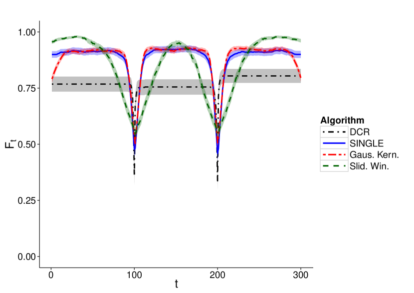
In order to obtain a general overview of the performance of the SINGLE algorithm we simulate data sets with the following structure: each data set consists of 3 segments each of length 100 (i.e., overall duration of 300). The correlation structure for each segment was randomly generated using an Erdős-Rényi random graph. Finally a VAR process for each corresponding correlation structure was simulated. Thus each data set consists of 2 change points at times and 200 respectively resulting in a network structure that is piece-wise constant over time. For this simulation the random graphs were generated with 10 nodes and the probability of an edge between two nodes was fixed at (i.e., the expected number of edges is ).
In the case of the SINGLE algorithm the value of was estimated by maximising the leave-one-out log-likelihood given in equation (19). Values of and were estimated by minimising AIC. For the DCR algorithm, the block size for the block bootstrap permutation tests to be 15 and one thousand permutations where used for each permutation test. In the case of the sliding window and Gaussian kernel algorithms the kernel width was estimated using leave-one-out log-likelihood and was estimated by minimising AIC.
In Figure [3] shows the average scores for each of the four algorithms over 500 simulations. We can see that the SINGLE algorithm performs competitively relative to the other algorithms. Specifically we note that the performance of the SINGLE algorithm mimics that of the Gaussian kernel algorithm. We also note that all four algorithms experience a dramatic drop in performance in the vicinity of change points. This effect is most pronounced for the sliding window algorithm.
3.2.2 Simulation \@slowromancapi@b - Scale-free networks
It has been reported that brain networks are scale-free, implying that their degree distribution follows a power law. From a biological perspective this implies that there are a small but finite number of hub regions which have access to most other regions (Eguiluz et al., 2005). While Erdős-Rényi random graphs offer a simple and powerful model from which to simulate random networks they fail to generate networks where the degree distribution follows a power law. In this simulation we analyse the performance of the SINGLE algorithm by simulating random networks according to the Barabási and Albert (1999) preferential attachment model. Here the power of preferential attachment was set to one. Additionally, edge strength was also simulated according to a uniform distribution on , introducing further variability in the estimated networks.
In Figure [4] we see the average scores for each of the four algorithms over 500 simulations. We note that the performance of the SINGLE and DCR algorithms is largely unaffected by the increased complexity of the simulation. This is not true in the case of the sliding window and Gaussian kernel algorithms, both of which see their performance drop. We attribute this drop in performance to the fall in the signal-to-noise ratio and to the increased complexity of the network structure. Similar results confirming that networks with skewed degree distributions (e.g., power-law distributions) are typically harder to estimate have also been described in Peng et al. (2009). Finally,
3.2.3 Simulation \@slowromancapi@c - Small-world networks
It has been widely reported that brain networks have a small-world topology (Stephan et al., 2000; Sporns et al., 2004; Bassett and Bullmore, 2006). In this simulation, multivariate time series were simulated such that the correlation structure follows a small-world graph according to the Watts-Strogatz model (Watts and Strogatz, 1998). Starting with a regular lattice, this model is parameterised by which quantifies the probability of randomly rewiring an edge. This results in networks where there is a tendency for nodes to form clusters, formally referred to as a high clustering coefficient. Both anatomical (Sporns et al., 2004) as well as the functional brain networks have been reported as exhibiting such a network topology (Bassett and Bullmore, 2006). Throughout this simulation we set and edge strength was simulated according to a Uniform distribution on .
In Figure [5] we see the average scores for each of the four algorithms over 500 simulations. We note that there is a clear drop in the performance of all the algorithms relative to their performance in simulations \@slowromancapi@a and \@slowromancapi@b. We believe this is due to the increased complexity of small-world networks compared to the previous networks we had considered. Formally, due to the high local clustering present in small-world networks, the path length between any two nodes is relatively short. As a result, we expect there to be a large number of correlated variables that are not directly connected. It has been reported that the Lasso (and therefore by extension the Graphical Lasso) cannot guarantee consistent variable selection in the presence of highly correlated predictors (Zou and Hastie, 2005; Zou, 2006). Since all four algorithms are related to the Graphical Lasso, we conjecture that this may be the cause of the overall drop in performance.
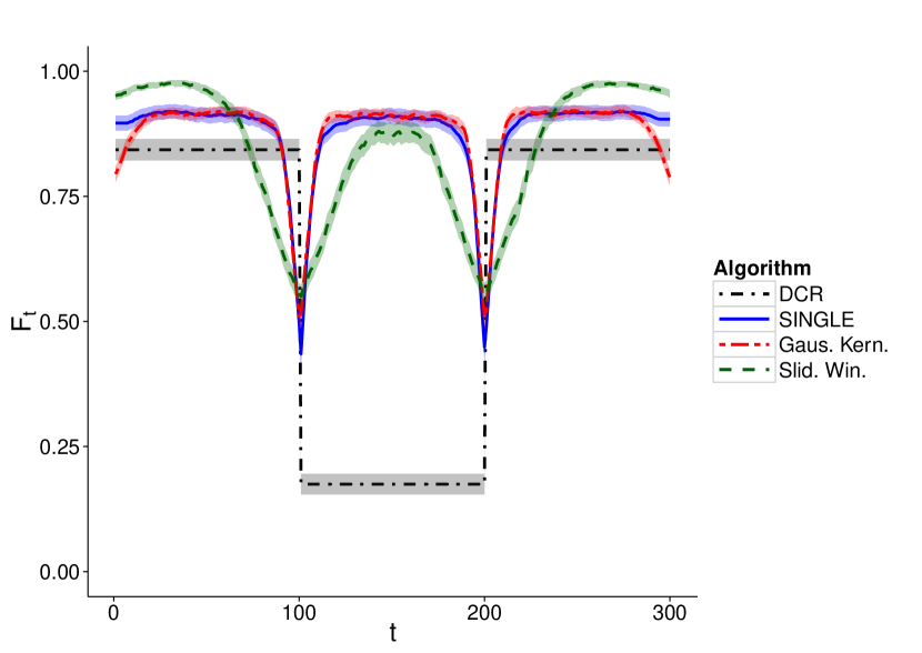
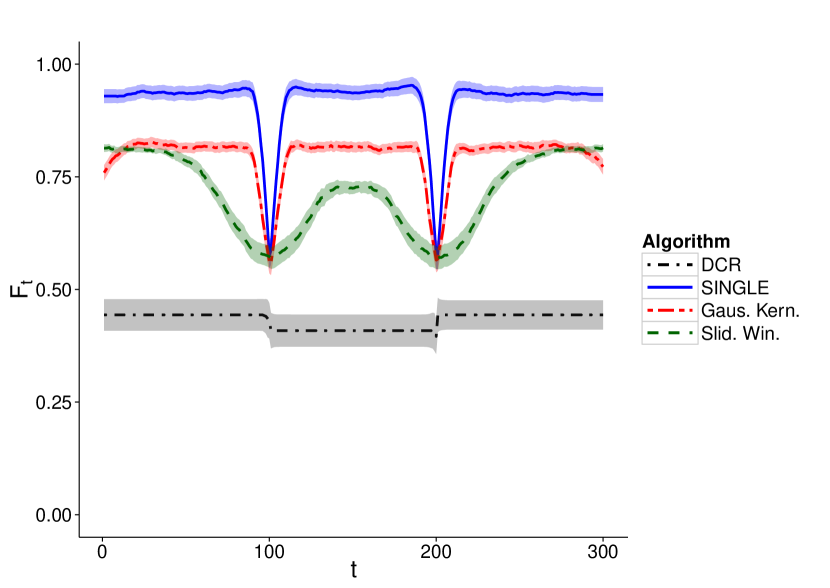
3.2.4 Simulation \@slowromancapii@a - Cyclic Erdős-Rényi networks
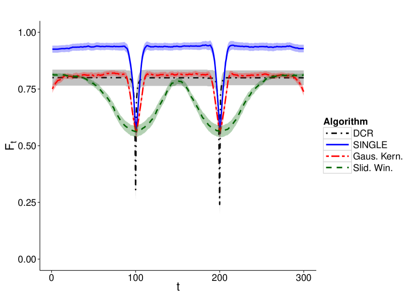
In task related experiments subjects are typically asked to alternate between performing a cognitive task and resting. As a result, we expect the functional connectivity structure to alternate between two states: a task related state and the resting state. In order to recreate this scenario, network structures are simulated in a cyclic fashion such that the first and third correlation structures are identical.
We note from Figure [6] that the performance of the SINGLE sliding window and Gaussian kernel algorithms is largely unaffected. However the DCR algorithm suffers a clear drop in performance relative to simulation \@slowromancapi@a. The drop in performance of the DCR algorithm is partly due to the presence of the recurring correlation structure. More specifically, we believe the problem to be related to the use of block bootstrapping permutation test to determine the significance of change points in the DCR. This test assumes that local data points are correlated but expects data points that are far away to be independent. Typically this assumption holds. However when there is a recurring correlation structure, points that are far away may follow the same underlying distribution. As a result the power of the permutation test is heavily reduced.
3.2.5 Simulation \@slowromancapii@b - Cyclic Scale-free networks
In this simulation we simulate multivariate time series where the underlying correlation structure is cyclic and follows a scale-free distribution. The results are summarised in Figures [7]. As in simulation \@slowromancapi@b there is no noticeable difference in the performance of the SINGLE algorithm. There is however a drop in the performance of the sliding window, Gaussian kernel and DCR algorithms. This is particularly evident in the case of the DCR algorithm. As mentioned previously the drop in performance of the sliding window and Gaussian kernel algorithms is due to the increased complexity of the network structure as well as the fall in the signal to noise ratio. In the case of the DCR the drop in performance can be partly explained by the fact the assumptions behind the use of the block bootstrap no longer hold (see simulation \@slowromancapii@a for a discussion) and the increased complexity of the network structure. These two factors combine to greatly affect the performance of the DCR algorithm.
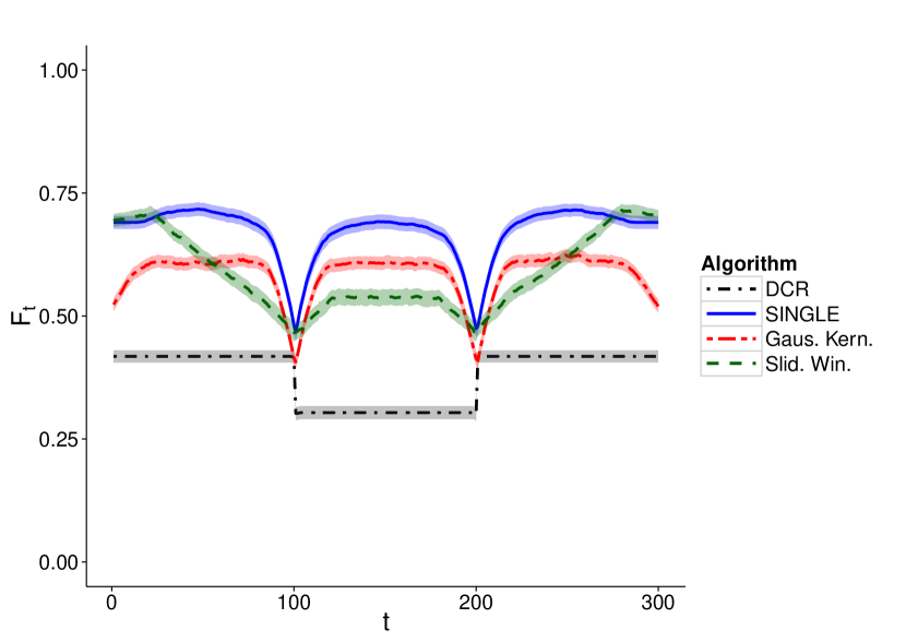
3.2.6 Simulation \@slowromancapii@c - Cyclic Small-world networks
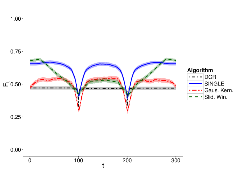
In this simulation we look to assess the performance of the SINGLE algorithm in a scenario that is representative of the experimental data we use in this work. As described previously, the experimental data used in this study corresponds to fMRI data from a Choice Reaction Time (CRT) task. Here subjects are required to make rapid visually-cued motor decisions. Stimulus was presented in five on-task blocks each preceding a period where subjects were at rest. As a result we expect there to be a cyclic network structure.
Thus in this simulation network structures are simulated in a cyclic fashion where each network structure is simulated according to a small-world network as in Simulation \@slowromancapi@c. This simulation gives us a clear insight into the performance of the SINGLE algorithm in a scenario that is very similar to that proposed in the experimental data.
The results are summarised in Figure [8]. We note that as in Simulation \@slowromancapi@c there is drop in the performance of all four algorithms relative to their performance in simulations \@slowromancapii@a and \@slowromancapii@b. We believe this is due to the increased complexity of the underlying networks structures, specifically the high levels of clustering we experience in small-world networks which are not seen in Erdős-Rényi or scale-free random networks.
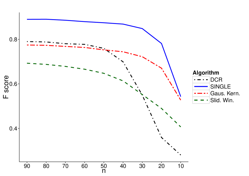
3.2.7 Simulation \@slowromancapiii@a - Scale-free networks with decreasing ratio
Here we study the behaviour of the proposed algorithm as the ratio of observations, , to the number of nodes, , decreases. This is a particularly relevant problem in the case of fMRI data as it is often the case that the number of nodes in the study (typically the number of ROIs) will be much larger than the number of observations.
In this simulation we fix and allow the value of to decrease. Here we simulate a data set with three segments each of length where the connectivity structure within each segment is randomly simulated according to a small-world network. Thus as the value of decreases we are able to quantify the performance of the SINGLE algorithm in the presence of rapid changes in network structure.
In the case of the SINGLE, sliding window and Gaussian kernel algorithms all parameters are estimated as discussed previously. In the case of the DCR algorithm the value of block sizes for the block bootstrap test was also reduced accordingly.
Results for Simulation \@slowromancapiii@a are given in Figure [9]. Error bars have been removed in the interest of clarity however detailed results are available in Table [3]. We note that all four algorithms struggle when is small relative to . This is to be expected as the number of observations is much smaller than the number of parameters to be estimated. Figure [9] shows that the performance of the SINGLE algorithm quickly improves as increases at a rate which is similar to that of the sliding window and Gaussian kernel algorithms.
| 10 | 0.28 | 0.09 |
|---|---|---|
| 20 | 0.36 | 0.15 |
| 30 | 0.55 | 0.21 |
| 40 | 0.70 | 0.15 |
| 50 | 0.76 | 0.08 |
| 60 | 0.78 | 0.07 |
| 70 | 0.78 | 0.06 |
| 80 | 0.79 | 0.03 |
| 90 | 0.79 | 0.02 |
| 10 | 0.54 | 0.13 |
|---|---|---|
| 20 | 0.78 | 0.08 |
| 30 | 0.85 | 0.06 |
| 40 | 0.87 | 0.05 |
| 50 | 0.87 | 0.05 |
| 60 | 0.88 | 0.05 |
| 70 | 0.89 | 0.04 |
| 80 | 0.89 | 0.04 |
| 90 | 0.89 | 0.04 |
| 10 | 0.53 | 0.09 |
|---|---|---|
| 20 | 0.67 | 0.07 |
| 30 | 0.72 | 0.05 |
| 40 | 0.74 | 0.05 |
| 50 | 0.75 | 0.04 |
| 60 | 0.76 | 0.04 |
| 70 | 0.77 | 0.03 |
| 80 | 0.77 | 0.03 |
| 90 | 0.77 | 0.03 |
| 10 | 0.41 | 0.09 |
|---|---|---|
| 20 | 0.49 | 0.10 |
| 30 | 0.55 | 0.10 |
| 40 | 0.61 | 0.09 |
| 50 | 0.65 | 0.07 |
| 60 | 0.67 | 0.07 |
| 70 | 0.68 | 0.06 |
| 80 | 0.69 | 0.05 |
| 90 | 0.69 | 0.05 |
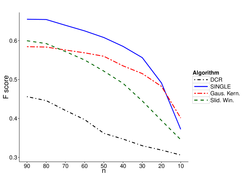
3.2.8 Simulation \@slowromancapiii@b - Small-world networks with decreasing ratio
As with Simulation \@slowromancapiii@a, we evaluate the performance of the proposed algorithm as the ratio of observations, , relative to the dimensionality of the data, , decreases. However, here the underlying network structure are simulated according to small-world networks. This simulation therefore provides an insight into how accurately proposed algorithm is able to estimate networks in the presence of rapid changes.
Results for Simulation \@slowromancapiii@b are given in Figure [10] and detailed results are provided in Table [4]. As with the previous simulations we note that the performance of all four algorithms is affected by the presence of small-world networks (see simulation \@slowromancapi@c for a discussion). Furthermore, as in simulation \@slowromancapiii@a, the performance of all four algorithms also deteriorates as the ratio decreases. Moreover, as in simulation \@slowromancapiii@a, the performance of the SINGLE algorithm improves as increases.
| 10 | 0.31 | 0.06 |
|---|---|---|
| 20 | 0.32 | 0.07 |
| 30 | 0.33 | 0.08 |
| 40 | 0.35 | 0.10 |
| 50 | 0.36 | 0.11 |
| 60 | 0.40 | 0.12 |
| 70 | 0.42 | 0.11 |
| 80 | 0.45 | 0.10 |
| 90 | 0.46 | 0.10 |
| 10 | 0.37 | 0.08 |
|---|---|---|
| 20 | 0.49 | 0.07 |
| 30 | 0.56 | 0.07 |
| 40 | 0.59 | 0.07 |
| 50 | 0.61 | 0.07 |
| 60 | 0.62 | 0.07 |
| 70 | 0.64 | 0.07 |
| 80 | 0.65 | 0.06 |
| 90 | 0.65 | 0.06 |
| 10 | 0.40 | 0.06 |
|---|---|---|
| 20 | 0.48 | 0.05 |
| 30 | 0.52 | 0.05 |
| 40 | 0.54 | 0.05 |
| 50 | 0.56 | 0.05 |
| 60 | 0.57 | 0.05 |
| 70 | 0.58 | 0.05 |
| 80 | 0.58 | 0.05 |
| 90 | 0.58 | 0.05 |
| 10 | 0.35 | 0.07 |
|---|---|---|
| 20 | 0.39 | 0.08 |
| 30 | 0.44 | 0.08 |
| 40 | 0.49 | 0.09 |
| 50 | 0.52 | 0.08 |
| 60 | 0.55 | 0.07 |
| 70 | 0.57 | 0.07 |
| 80 | 0.59 | 0.06 |
| 90 | 0.60 | 0.06 |
3.2.9 Computational Cost
From a practical perspective we are also interested in the computational cost of the SINGLE algorithm. While this has already been discussed previously we look to benchmark the computational cost of the SINGLE algorithm relative to the previously considered algorithms.
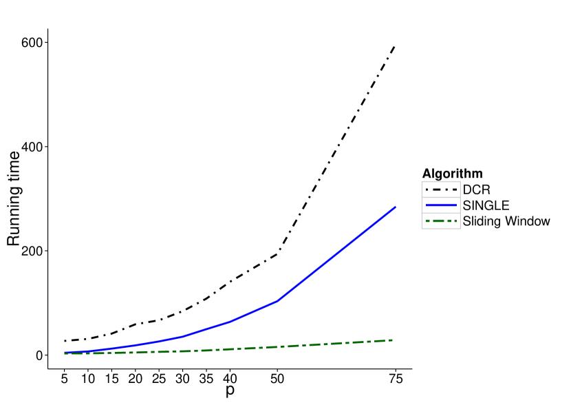
As noted in section 2.2.2, the limiting factor in the computational cost of the SINGLE algorithm is the number of nodes, . We note that this is also the case for the sliding window, Gaussian kernel and DCR algorithms (see Appendix F). As a result we compare the running times of each of the algorithms as increases for fixed .
Here each data set was simulated in the same manner as in Simulation \@slowromancapi@c. That is, each dataset consisted of 3 segments of length 100 (resulting in an overall duration of 300). The correlation structure within each segment was then randomly generated according to small-world network.
In Figure [11] we plot the mean running time of each algorithm over 50 iterations for increasing . It is clear that the computational cost of the SINGLE algorithm increases exponentially with . However we note that for nodes the algorithm can still be run in under 5 minutes, making it practically feasible. This simulation was run on a computer with an Intel Core i5 CPU at 2.8 GHz.
4 Application to a Choice Reaction Time (CRT) task fMRI dataset
In this section we assess the ability of the SINGLE algorithm when detecting changes in real fMRI data evoked using a simple cognitive task, the Choice Reaction Time (CRT) task. The CRT is a forced choice visuo-motor decision task that reliably activates visual, motor and many cognitive control regions. The task was blocked into alternating task and rest periods. As a result we expect the task onset to evoke an abrupt change in the correlation structure that is cyclical in nature.
This is a highly challenging data set for several reasons. Firstly, it corresponds to the scenario where is small. Secondly, there is a high rate of change in the correlation structure with a change in cognitive state roughly every 15 seconds. Finally, given the nature of the CRT task there is a recurring correlation structure with subjects alternating between two cognitive states: resting and performing the CRT task. As we have seen in the simulations the SINGLE algorithm is well equipped to handle the aforementioned challenges.
In order to study the roles of the various ROIs during the CRT task we consider the changes in betweenness centrality of each node over time. The betweenness centrality of a node is the sum of how many shortest paths between all other nodes pass through it (Pandit et al., 2013). Nodes with high betweenness centralities are considered to be of important, hub nodes in the network (Hagmann et al., 2008).
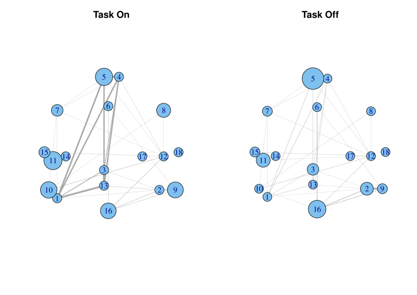
As described previously the CRT task involves subjects alternating between performing a visual stimulus task (on task) and resting state (off task). Figure [12] shows the average estimated functional connectivity networks for a patient on and off task respectively. Here the size of each node is proportional to the sum of the betweenness centralities of the corresponding ROI and the edge thickness is proportional to the partial correlation between nodes. We notice that the on task network is appears to be more focused that the off task network and this can also be seen in the corresponding example video provided in the supplementary material.
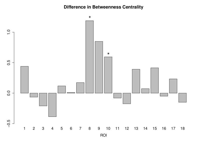
We note that there are changes in the betweenness centralities of several nodes between tasks. In order to determine the significance of any changes betweenness centrality as a result of the changing cognitive state of the subjects we study the estimated graphs for each of the 24 subjects both on and off task. Figure [13] shows the percentage change in betweenness centrality from off task to on task for each ROI. To determine the statistical significance of reported changes a Wilcoxon rank sum test was employed. The resulting -values where adjusted according to the Bonferroni-Holm method in order to account for multiple tests. The results indicated that at the level there was a statistically significant increase in betweenness centrality for the 8th (Right Inferior Frontal Gyrus) and 10th (Right Inferior Parietal) ROIs. This indicates that during this simple, cognitive task the Right Inferior Frontal Gyrus and the Right Inferior Parietal become more hub-like. This is particularly true in the case of the Right Inferior Frontal Gyrus where the change in betweenness centrality is particularly sizeable.
These findings suggest that the Right Inferior Frontal Gyrus and Right Inferior Parietal play a key role in cognitive control and executive functions as demonstrated by their dynamically changing betweenness centrality throughout the task. This result agrees with the proposed functional roles for the Right Inferior Frontal Gyrus (and adjacent right anterior insula), which is assumed to play a fundamental role in attention and executive function during cognitively demanding tasks and may have an important role in regulating the balance between other brain regions (Aron et al., 2003; Hampshire et al., 2010; Bonnelle et al., 2012). The findings also agree with the proposed function of the Right Inferior Parietal lobe, which has been reported to play a role in high-level cognition (Mattingley et al., 1998) and sustaining attention (Corbetta and Shulman, 2002; Husain and Nachev, 2007).
One possible interpretation of the the increase in betweenness centrality is that the Right Inferior Frontal Gyrus becomes more important for the flow of information around the brain during the more challenging cognitive task.
5 Discussion
In this work we introduce the Smooth Incremental Graphical Lasso Estimation (SINGLE) algorithm, a new methodology for estimating sparse dynamic functional connectivity networks from non-stationary fMRI data. Our approach provides two main advantages. First, the proposed algorithm is able to accurately estimate functional connectivity networks at each observation. This allows for the quantification the dynamic behaviour of brain networks at a high temporal granularity. The second advantage lies in the SINGLE algorithm’s ability to quantify network variability over time. In SINGLE, networks are estimated simultaneously in a unified framework which encourages temporal homogeneity. This results in networks with sparse innovations in edge structure over time and implies that changes in connectivity structure are only reported when substantiated by evidence in the data. Although the use of the SINGLE algorithm is particularly suitable for task related experiments, there is also a growing body of evidence to suggest that functional connectivity is highly non-stationary even in resting state, making the SINGLE algorithm these studies as well.
The SINGLE algorithm is closely related to sliding window based algorithms. We note that Zhou et al. (2010) have extensively studied the combined use of kernel methods and constrained optimisation to estimate dynamic networks and provide a theoretical guarantee that accurate estimates of time varying network structure can be obtained in such a manner under mild assumptions. The approach taken there is to estimate sample covariance matrices at each using kernel methods with the Graphical Lasso being used subsequently to estimate the corresponding precision matrices. However, given time points this approach corresponds directly to independent iterations of the Graphical Lasso. As a result, while smooth estimates of the sample covariance matrix are obtained via the use of kernels, there is no mechanism in place to enforce temporal homogeneity in the corresponding precision matrices. Consequently the estimated partial correlations may not accurately represent the functional connectivity over time. The SINGLE algorithm addresses precisely this problem by directly enforcing temporal homogeneity. This is achieved via the introduction an additional constraint inspired by the Fused Lasso. As shown in our simulation study, this additional constraint results in higher accuracy of estimated networks in a vast array of scenarios.
The SINGLE algorithm requires the input of 3 parameters, and , each of which has a natural interpretation for the user. Penalty parameters and enforce sparsity and temporal homogeneity respectively. They can be tuned by minimising over a given range of values. The choice of can be interpreted as the window length and we provide an data-driven method for tuning parameter using the leave-one-out log-likelihood. We note that the choice of is a delicate matter as well as an active area of research in its own right. The choice of can be seen as a trade-off between stability and temporal adaptivity. Setting to be too large will result in network estimates that resemble the global mean and omit valuable short-term fluctuations in connectivity structure. Conversely, setting to be too small will lead to networks that are dominated by noise. Given this reasoning, it is often desirable to have a kernel width which is dependent on the location within the time series. This allows the kernel width to decrease in the proximity of a change-point (allowing for rapid temporal adaptivity) and increase when data is piece-wise stationary (in order to fully exploit all relevant data). The idea of adaptive values of has been studied in literature such as Haykin (2002) and Príncipe et al. (2011), however, we leave this for future work.
Our simulation results indicate that the SINGLE algorithm can accurately estimate the true underlying functional connectivity structure when provided with non-stationary multi-variate time series data. We identify three relevant scenarios where the proposed method performs competitively. The first, demonstrated by simulation \@slowromancapi@, quantifies our claim that the SINGLE algorithm is able to accurately estimate dynamic functional connectivity networks. In task based experiments it is often the case that tasks are repetitively performed followed by a period of rest, resulting in the presence of a cyclic functional connectivity structure. This scenario is studied in simulation \@slowromancapii@ which serves as an indication that the SINGLE algorithm is not adversely affected in such cases. Furthermore, we have shown that the SINGLE algorithm is relatively robust when the ratio of observations to nodes falls, meaning that the SINGLE algorithm can be applied on a subject-by-subject basis. This is a great advantage as it avoids the issue of subject-to-subject variability and allows for the estimation of functional connectivity networks for each subject. This potentially allows for estimated dynamic connectivity to be used to differentiate between subjects. Finally, the computational cost of the proposed algorithm is studied empirically in simulation \@slowromancapiv@. A summary of all the simulation results is provided in Table [5].
| SINGLE | DCR | Sliding window/Gaussian kernel | |
|---|---|---|---|
| Temporal adaptivity | |||
| Temporal homogeneity | X | ||
| Cyclic correlation structure | X | ||
| Parameters | |||
| Computational Complexity |
We do note that the performance of the SINGLE algorithm was affected by the presence of small-world network structure. We believe this may be caused by the high local clustering present in such networks. This results in the short minimum path lengths between many nodes. This would cause there be a large number of correlated nodes which are not directly connected. It has been reported that the Lasso (and by extension the Graphical Lasso) cannot guarantee consistent variable selection in the presence of highly correlated predictors (Zou and Hastie, 2005; Zou, 2006). This issue has recently been studied in the context of genetic networks by Peng et al. (2009) and in future these approaches could be adapted to address such issues.
We have presented an application showing that the SINGLE algorithm can detect cyclical changes in network structure with fMRI data acquired while subjects perform a simple cognitive task and identify the Right Inferior Frontal Gyrus as well as the Right Inferior Parietal as changing their graph theoretic properties as the functional connectivity network reorganises. We find that there is a significant increase in the betweenness centrality for both these regions. These findings suggest that the Right Inferior Frontal Gyrus together with the Right Inferior Parietal play a key role in cognitive control and the functional reorganisation of brain networks. In the case of the Right Inferior Frontal Gyrus, this result agrees with the proposed functional roles of the Right Inferior Frontal Gyrus (Aron et al., 2003; Corbetta and Shulman, 2002; Hampshire et al., 2010; Bonnelle et al., 2012). The Right Inferior Parietal lobe has also been reported to play a role in high-level cognition (Mattingley et al., 1998) and sustaining attention (Corbetta and Shulman, 2002; Husain and Nachev, 2007). One possible interpretation is that both the Right Inferior Frontal Gyrus and the Right Inferior Parietal become more important to the flow of information during the more challenging cognitive task as demonstrated by their rise in betweenness centrality.
In conclusion, the SINGLE algorithm provides an alternative and novel method for estimating the underlying network structure associated with dynamic fMRI data. It is ideally suited to analysing data where a change in the correlation structure is expected but little more is known. Going forward, the SINGLE algorithm can be applied to different types of fMRI data sets, exploring different cognitive tasks such as those with multiple task demands, exploring how networks change with more subtle differences in cognitive state (i.e., rather than just task on or off). Similarly, the approach can be used to investigate spontaneous network reorganisation in the resting state and compare this across different subject groups (e.g., comparing pathological states with healthy controls). From a methodological point of view it would be interesting to consider variations of the SINGLE objective function, particularly with respect to the Fused Lasso component of the penalty. For example, this component could be exchanged with a trend filtering penalty (Kim et al., 2009).
Appendix
Here we formally derive some of the results discussed in the main text. Throughout this section we assume the following results relating to convex functions:
-
(1)
A function is convex if and only if the function where
is convex in for all and .
Here we write to denote the domain of function . -
(2)
Assuming is twice differentiable (i.e., its Hessian exists for all ) then will be convex if and only if its Hessian is positive semidefinite.
-
(3)
The composition of convex functions is itself a convex function
-
(4)
Any norm is convex (this follows from the definition of a norm and the triangle inequality)
-
(5)
The sum of convex functions is convex
A The SINGLE objective function given in equation (3) is convex
Recall the SINGLE cost function was defined as:
| (23) |
From Assumption (5) it suffices to show that each component of is convex. Furthermore from Assumptions (3) and (4) it follows that and are convex for all and . We note that . Therefore is an affine function for all as it is a linear sum. Finally we come to . It follows that showing that is convex is equivalent to showing that is concave. In order to do so we use Assumption (1). Formally we define as , where refers to the set of positive semi-definite by matrices. We also define for all . Since is positive semi-definite it follows that has a square root . Thus in order to show that is concave we can rewrite as follows:
Thus we have that .
Now we can take the eigendecomposition of where is an orthonormal matrix of eigenvectors and is a diagonal matrix where the th entry along the diagonal is the th eigenvalue, . Finally we note that:
By differentiating and using Assumption (2) we note that is concave and thus conclude that is concave and that the SINGLE cost function is convex.
B The scaled augmented Lagrangian corresponding to equations (7) and (8) is given by as shown in equation (9).
In the case of equations (7-8) the corresponding Lagrangian is given by:
| (24) |
where are Lagrange multipliers or dual variables. The final term in the Lagrangian is equivalent to the sum of all elements in the matrix .
The augmented Lagrangian is essentially composed of the original Lagrangian and an additional penalty term. In our case the augmented Lagrangian is given by:
| (25) |
We can simplify equation (25) by noting that is equivalent to the elementwise sum of entries of the matrix where denotes the elementwise multiplication of matrices. Thus we can combine the linear and quadratic constraint terms as follows:
| (26) | ||||
| (27) |
where are the scaled Lagrange multipliers. This yields the scaled augmented Lagrangian given in equation (25).
C If symmetric matrices satisfy for some constant then it follows that and have the same eigenvectors. Furthermore it is also the case that the th eigenvectors of and , denoted by and respectively, will satisfy for
In order to prove claim 2 we begin taking the eigendecompositions of and as and respectively. Substituting these into we obtain:
Expanding the left hand side yields:
where we have made us of the fact that is an orthonormal matrix. Thus it follows that and since both and are diagonal matrices we also have that for
D Each of the optimisations of the form given in equation (16) can be solved by applying the Fused Lasso Signal Approximator.
The Lasso is a regularised regression method that selects a sparse subset of predictors in least squares estimation. That is, the Lasso minimises the following objective function:
where is the response vector, is the matrix of predictors and is a vector of coefficients. The Fused Lasso extends the Lasso under the assumption that there is a natural ordering to the coefficients . The Fused Lasso is able to do so by adding an additional penalty to the Lasso objective function as follows:
Here only adjacent coefficients and are penalised but the Fused Lasso objective function can be specified to as to induce sparsity between any subset of . A special case of the Fused Lasso occurs when . In this case the penalty results in being a piece-wise continuous approximation to . We note that equation (16) resembles the objective function of the Fused Lasso. This can be seen by setting and for .
E The dual update in Step 3 guarantees dual feasibility in the variables and dual feasibility in the variables can be checked by considering .
This result is taken from Boyd et al. (2010). Consider the general (unscaled) augmented Lagrangian with arbitrary matrices , and :
All solutions must satisfy the following constraints:
| Primal feasibility: | |||
| Dual feasibility: |
where dual feasibility is based on the unscaled, unaugmented Lagrangian.
The ADMM algorithm iteratively minimises and such that at iteration we obtain that minimises . From this it follows that:
Thus it follows that by setting dual feasibility in the variable is guaranteed. Finally, after rescaling by and noting that in the SINGLE algorithm and we get the update in step 3.
Now we can continue to consider criteria for confirming dual feasibility in terms of variables. Since we are guaranteed dual feasibility in variables we only need to check for dual feasibility in variables. Since minimises we have:
Thus in order to have dual feasibility in variables we require
Since in our case we have that and it follows that we can check for dual feasibility by considering .
F The computational complexity of the DCR algorithm is where is the number of bootstrap permutations to perform
We begin by noting that the computational complexity of the Graphical Lasso is . While it is possible to reduce the computational complexity in some special cases we do not consider this below.
Prior to outlining our proof, a brief overview of the DCR algorithm is in order. The DCR algorithm looks to estimate dynamic functional connectivity networks by segmenting data into piece-wise continuous partitions. Within each partition the network structure is assumed to be stationary, allowing for the use of a wide variety of network estimation algorithms. In the case of the DCR the Graphical Lasso is chosen.
The data, , is segmented using a greedy partitioning scheme. Here the global network is first estimated using the Graphical Lasso. The BIC of the global network is noted and subsequently used to propose change-points. The DCR algorithm then proceeds to partition the data into subsets and for . Thus represents the minimum number of observations between change-points.
For each of these partitions a network is estimated for and and their joint BIC is noted. This step therefore involves iterations of the Graphical Lasso, resulting in a computation complexity of .
Subsequently, the value of resulting in the greatest reduction in BIC relative to the global network is proposed as a change-point. In order to check the statistical significance of the proposed change-point a block bootstrap permutation permutation test is performed. This step involves a further iterations of the Graphical Lasso where is the number of bootstrap permutations performed. As a result this step has a computational complexity of .
This procedure is repeated until all significant change-points have been reported. We therefore conclude that the computational complexity of the DCR algorithm is .
References
- Achard et al. [2006] S. Achard, R. Salvador, B. Whitcher, J. Suckling, and E. T. Bullmore. A resilient, low-frequency, small-world human brain function network with highly connected association of cortical hubs. Journal of Neuroscience, 26(1):63–72, 2006.
- Aron et al. [2003] A. R. Aron, P. C. Fletcher, E. T. Bullmore, B. J. Sahakain, and T. W. Robbins. Stop-signal inhibition disrupted by damage to right inferior frontal gyrus in humans. Nature Neuroscience, 2003.
- Barabási and Albert [1999] A. Barabási and R. Albert. Emergence of scaling in random networks. Science, 286(5439):509–512, 1999.
- Bassett and Bullmore [2006] D. Bassett and E. Bullmore. Small-world brain networks. The Neuroscientist, 12(6):512–523, 2006.
- Bertsekas [1999] D. P. Bertsekas. Nonlinear programming. Athena Scientific, 1999.
- Bonnelle et al. [2012] V. Bonnelle, T. E. Ham, R. Leech, K. M. Kinnunen, M. A. Mehta, R. J. Greenwood, and D. J. Sharp. Salience network integrity predicts default mode network function after traumatic brain injury. Proceedings of the National Academy of Sciences, 109(12):4690–4695, 2012.
- Boyd et al. [2010] S. Boyd, N. Parikh, E. Chu, B. Peleato, and J. Eckstein. Distributed Optimization and Statistical Learning via the Alternating Direction Method of Multipliers. Foundations and Trends in Machine Learning, 3(1):1–122, 2010.
- Bullmore and Sporns [2009] E. Bullmore and O. Sporns. Complex brain networks: graph theoretical analysis of structural and functional systems. Nature, 10:186–198, 2009.
- Calhoun et al. [2009] V. D. Calhoun, J. Liu, and T. Adalı. A review of group ICA for fMRI data and ICA for joint inference of imaging, genetic, and ERP data. NeuroImage, 45(1):S163–S172, 2009.
- Chang and Glover [2010] C. Chang and G. H. Glover. Time frequency dynamics of resting-state brain connectivity measured with fMRI. NeuroImage, 50(1):81 – 98, 2010.
- Corbetta and Shulman [2002] M. Corbetta and G. L. Shulman. Control of goal-directed and stimulus-driven attention in the brain. Nature Reviews Neuroscience, 3(3):201–215, 2002.
- Cribben et al. [2012] I. Cribben, R. Haraldsdottir, Y. L. Atlas, T. D. Wager, and M. A Lindquist. Dynamic Connectivity Regression: Determining state-related changes in brain connectivity. NeuroImage, 61(4):907–920, 2012.
- Danaher et al. [2013] P. Danaher, P. Wang, and D. Witten. The Joint Graphical Lasso for Inverse Covariance Estimation across Multiple Classes. Journal of the Royal Statistical Society: Series B (Statistical Methodology), 76(2):373–397, 2013.
- Duchi and Singer [2009] J. Duchi and Y. Singer. Efficient online and batch learning using forward backward splitting. The Journal of Machine Learning Research, 10:2899–2934, 2009.
- Eguiluz et al. [2005] V. M. Eguiluz, D. R. Chialvo, G. A. Cecchi, M. Baliki, and A. V. Apkarian. Scale-free brain functional networks. Physical review letters, 94(1):018102, 2005.
- Erdos and Renyi [1959] P. Erdos and A. Renyi. On random graphs. Publicationes Mathematicae Debrecen, 1959.
- Esposito et al. [2003] F. Esposito, E. Seifritz, E. Formisano, R. Morrone, T. Scarabino, G. Tedeschi, S. Cirillo, R. Goebel, and F. Di Salle. Real-time independent component analysis of fMRI time-series. NeuroImage, 20(4):2209–2224, 2003.
- Esposito et al. [2006] F. Esposito, A. Bertolino, T. Scarabino, V. Latorre, G. Blasi, T. Popolizio, G. Tedeschi, S. Cirillo, R. Goebel, and F. Di Salle. Independent component model of the default-mode brain function: Assessing the impact of active thinking. Brain Research Bulletin, 70(4):263–269, 2006.
- Fair et al. [2009] D. A. Fair, A. L. Cohen, J. D. Power, N. U. Dosenbach, J. A. Church, F. M. Meizin, B. L. Schlaggar, and S. E. Petersen. Functional Brain Networks Develop from a “Local to Distributed” Organization. PloS, 5(5), 2009.
- Fornito et al. [2012] A. Fornito, B. J. Harrison, A. Zalesky, and J. S. Simons. Competitive and cooperative dynamics of large-scale brain functional networks supporting recollection. Proceedings of the National Academy of Sciences, 109(31):12788–12793, 2012.
- Fornito et al. [2013] A. Fornito, A. Zalesky, and M Breakspear. Graph analysis of the human connectome: Promise, progress, and pitfalls. NeuroImage, 80:426–444, 2013.
- Fransson [2006] P. Fransson. How default is the default mode of brain function? further evidence from intrinsic bold signal fluctuations. Neuropsychologia, 44(14):2836–2845, 2006.
- Friedman et al. [2008] T. Friedman, T. Hastie, and R. Tibshirani. Sparse inverse covariance estimation via the Graphical Lasso. Biostatistics, 9(3):432–441, 2008.
- Friston [2011] K. J. Friston. Function and Effective Connectivity: A Review. Brain Connectivity, 1(1):13–36, 2011.
- Hagmann et al. [2008] P. Hagmann, L. Cammoun, X. Gigandet, R. Meuli, C. J Honey, V. J. Wedeen, and O. Sporns. Mapping the structural core of human cerebral cortex. PLoS Biology, 6(7):e159, 2008.
- Hampshire et al. [2010] A. Hampshire, S. R. Chamberlain, M. M. Monti, J. Duncan, and A. M. Owen. The role of the right inferior frontal gyrus: inhibition and attentional control. NeuroImage, 50(3):1313–1319, 2010.
- Handwerker et al. [2012] D. A. Handwerker, V. Roopchansingh, J. Gonzalez-Castillo, and P. A. Bandettini. Periodic changes in fMRI connectivity. NeuroImage, 63:1721–1719, 2012.
- Hastie et al. [2009] T. Hastie, R. Tibshirani, and J. Friedman. The Elements of Statistical Learning, volume 2. Springer, 2009.
- Haykin [2002] S. Haykin. Adaptive Filter Theory. Prentice Hall Information and System Science Series, 2002.
- Hellyer et al. [2014] P. J. Hellyer, M. Shanahan, G. Scott, R. J. S. Wise, D. J. Sharp, and R. Leech. The control of global brain dynamics: Opposing actions of frontoparietal control and default mode networks on attention. The Journal of Neuroscience, 34(2):451–461, 2014.
- Hinne et al. [2013] M. Hinne, L. Ambrogioni, R. J. Janssen, T. Heskes, and M. van Gerven. Structurally-informed bayesian functional connectivity analysis. NeuroImage, 86:294–305, 2013.
- Hoefling [2010] H. Hoefling. A path algorithm for the Fused Lasso Signal Approximator. Journal of Computational and Graphical Statistics, 19(4):984–1006, 2010.
- Huang et al. [2010] S. Huang, L. Sun, J. Ye, A. Fleisher, T. Wu, K. Chen, and E. Reiman. Learning brain connectivity of alzheimer’s disease by sparse inverse covariance estimation. NeuroImage, 50(3):935 – 949, 2010.
- Husain and Nachev [2007] M. Husain and P. Nachev. Space and the Parietal Cortex. Trends in Cognitive Sciences, 11(1):30–36, 2007.
- Hutchinson et al. [2012] M. R. Hutchinson, T. Womelsdoft, J. S. Gat, S. Everling, and R. S. Menon. Resting-state networks show dynamic functional connectivity in awake humans and anesthetized macaques. Human Brain Mapping, 34:2154–2177, 2012.
- Hutchinson et al. [2013] M. R. Hutchinson, T. Womelsdoft, P. A. Allen, E. A.Bandettini, V. D. Calhoun, M. Corbetta, S. D. Penna, J. Duyn, G. Glover, J. Gonzalez-Castillo, D. A. Handwerker, S. Keilholz, V. Kiviniemi, D. A. Leopold, F. de Pasquale, O. Sporns, M. Walterm, and C. Chang. Dynamic Functional Connectivity: Promise, issues, and interpretations. NeuroImage, 80:360–378, 2013.
- Kim et al. [2009] S-J Kim, K. Koh, S. Boyd, and D. Gorinevsky. l1 trend filtering. Siam Review, 51(2):339–360, 2009.
- Lindquist [2008] M. Lindquist. The statistical analysis of fMRI data. Statistical Science, 23(4):439–464, 2008.
- Liu et al. [2009] P Liu, Y. Zhang, K. Yuan, W. Qin, L. Zhou, J. Liang, P. Chen, J. Dai, Y. Liu, and J. Tian. Partial correlation investigation on the default mode network involved in acupuncture: An fMRI study. Neuroscience Letters, 462:183–187, 2009.
- Lowe et al. [1998] M. J. Lowe, B. J. Mock, and J. A. Sorenson. Functional connectivity in single and multislice echoplanar imaging using resting-state fluctuations. NeuroImage, 7:119–132, 1998.
- Markov et al. [2013] N. T. Markov, M. Ercsey-Ravasz, D. C. Van Essen, K. Knoblauch, Z. Toroczkai, and H. Kennedy. Cortical high-density counterstream architectures. Science, 342(6158), 2013.
- Marrelec et al. [2006] G. Marrelec, A. Krainik, H. Duffau, M. Pelegrini-Issac, S. Lehericy, J. Doyon, and H. Benali. Partial correlation for functional brain interactivity investigation in functional. NeuroImage, 32:228–237, 2006.
- Marrelec et al. [2009] G. Marrelec, J. Kim, J. Doyon, and B. Horwitz. Large-scale neural model validation of partial correlation analysis for effective connectivity investigation in functional MRI. Human brain mapping, 30(3):941–950, 2009.
- Mattingley et al. [1998] J. B. Mattingley, M. Husain, C. Rorden, C. Kennard, and J. Driver. Motor role of human inferior parietal lobe revealed in unilateral neglect patients. Nature, 392(6672):179–182, 1998.
- Monti et al. [2014] R. P. Monti, , G. Montana, and C. Anagnostopoulos. SINGLE: Estimate sparse dynamic graphs using the Smooth Incremental Graphical Lasso Estimation (SINGLE) algorithm, 2014. URL http://CRAN.R-project.org/package=SINGLE. R package version 1.2.
- Newman [2003] M. E. J. Newman. The structure and function of complex networks. SIAM Review, 45(2):167–256, 2003.
- Nichols and Hayasaka [2003] T. Nichols and S. Hayasaka. Controlling the familywise error rate in functional neuroimaging: a comparative review. Statistical Methods in Medical Research, 12(5):419–446, 2003.
- Pandit et al. [2013] A. S. Pandit, P. Expert, R. Lambiotte, V. Bonnelle, R. Leech, F. E. Turkheimer, and D. J. Sharp. Traumatic brain injury impairs small-world topology. Neurology, 80(20):1826–1833, 2013.
- Peng et al. [2009] J. Peng, P. Wang, N. Zhou, and J. Zhu. Partial correlation estimation by joint sparse regression models. Journal of the American Statistical Association, 104(486):735–746, 2009.
- Poldrack et al. [2011] R. A. Poldrack, J. A. Mumford, and T. E. Nichols. Handbook of Functional MRI Data Analysis. Cambridge University Press, 2011.
- Príncipe et al. [2011] J. C. Príncipe, W. Liu, and S. Haykin. Kernel Adaptive Filtering: A Comprehensive Introduction, volume 57. John Wiley & Sons, 2011.
- Sakoglu et al. [2010] U. Sakoglu, G. D. Pearlson, K. A. Kiehl, Y. M. Wang, A. M. Micheal, and V. D. Calhoun. A method for evaluating dynamic functional network connectivity and task modulation: application to schizophrenia. Magnetic Resonance Materials in Physics, Biology and Medicine, 23:351–366, 2010.
- Silverman [1986] B. W. Silverman. Density Estimation for Statistics and Data Analysis, volume 26. CRC press, 1986.
- Smith et al. [2004] S. M. Smith, M. Jenkinson, M. W. Woolrich, C. F. Beckmann, T. E. J. Behrens, H. Johansen-Berg, P. R. Bannister, De Luca M., I. Drobnjak, D. E. Flitney, R. K. Niazy, Saunders J., J. Vickers, Y. Zhang, N. De Stefano, M. J. Brady, and P. M. Matthews. Advances in functional and structural MR image analysis and implementation as FSL. NeuroImage, 23, Supplement 1(0):S208 – S219, 2004.
- Smith et al. [2011] S. M. Smith, K. L. Miller, S-K Gholamrez, M. Webster, C. F. Beckmann, T. E. Nichols, J. D. Ramsey, and M. W. Woolrich. Network modelling methods for fMRI. NeuroImage, 54(2):875 – 891, 2011.
- Sporns et al. [2004] O. Sporns, D. R. Chialvo, M. Kaiser, and C. C. Hilgetag. Organization, development and function of complex brain networks. Trends in Cognitive Sciences, 8(9):418–425, 2004.
- Stephan et al. [2000] K. E. Stephan, C. Hilgetag, G. Burns, M. A. O’Neill, M. P. Young, and R. Kotter. Computational analysis of functional connectivity between areas of primate cerebral cortex. Philosophical Transactions of the Royal Society of London. Series B: Biological Sciences, 355(1393):111–126, 2000.
- Strother et al. [1995] S. C Strother, J. R. Anderson, K. A. Schaper, J. J. Sidtis, J-S. Liow, R. P. Woods, and D. A. Rottenberg. Principal component analysis and the scaled subprofile model compared to intersubject averaging and statistical parametric mapping: I. ”functional connectivity” of the human motor system studied with O] water PET. Journal of Cerebral Blood Flow and Metabolism, 15:738–753, 1995.
- Sun et al. [2004] F. T. Sun, L. M. Miller, and M. D’Eposito. Measuring interregional functional connectivity using coherence and partial coherence analyses of fMRI data. NeuroImage, 21:647–658, 2004.
- Sun et al. [2007] F. T. Sun, L. M. Miller, A. A. Rao, and M. D’Esposito. Functional connectivity of cortical networks involved in bimanual motor sequence learning. Cerebral cortex, 17(5):1227–1234, 2007.
- Tibshirani et al. [2005] R. Tibshirani, M. Saunders, S. Rosset, J. Zhu, and K. Knight. Sparsity and smoothness via the fused lasso. Journal of the Royal Statistical Society Series B, 67(1):91–108, 2005.
- van der Heuvel and Hulshoff Pol [2010] M. P. van der Heuvel and H. E. Hulshoff Pol. Exploring the brain network: A review on resting-state fMRI functional connectivity. European Neuropsychopharmacology, 20(8):519 – 534, 2010.
- Watts and Strogatz [1998] D. J. Watts and S. H. Strogatz. Collective dynamics of small-world networks. Nature, 393(6684):440–442, 1998.
- Whittaker [1990] J. Whittaker. Graphical Models in Applied Multivariate Statistics. John Wiley and Sons, 1990.
- Xiao [2010] L. Xiao. Dual averaging methods for regularized stochastic learning and online optimization. Journal of Machine Learning Research, 11(2543-2596):4, 2010.
- Zhou et al. [2010] S. Zhou, J. Lafferty, and L. Wasserman. Time Varying Undirected Graphs. Machine Learning, 80:295–319, 2010.
- Zou [2006] H. Zou. The adaptive lasso and its oracle properties. Journal of the American Statistical Association, 101(476):1418–1429, 2006.
- Zou and Hastie [2005] H. Zou and T. Hastie. Regularization and variable selection via the Elastic Net. Journal of the Royal Statistical Society: Series B (Statistical Methodology), 67(2):301–320, 2005.