Stable commutator length in Baumslag–Solitar groups and quasimorphisms for tree actions

Abstract.

This paper has two parts, on Baumslag–Solitar groups and on general $G$–trees.

In the first part we establish bounds for stable commutator length (scl) in Baumslag–Solitar groups. For a certain class of elements, we further show that scl is computable and takes rational values. We also determine exactly which of these elements admit extremal surfaces.

In the second part we establish a universal lower bound of $1/12$ for scl of suitable elements of any group acting on a tree. This is achieved by constructing efficient quasimorphisms. Calculations in the group $BS(2,3)$ show that this is the best possible universal bound, thus answering a question of Calegari and Fujiwara. We also establish scl bounds for acylindrical tree actions.

Returning to Baumslag–Solitar groups, we show that their scl spectra have a uniform gap: no element has scl in the interval $(0,1/12)$.

1. Introduction

Stable commutator length has been the subject of a significant amount of recent work, especially by Danny Calegari and his collaborators. See [6] for an introduction to stable commutator length and a desciption of much of this work. A major breakthrough in this area was Calegari’s algorithm [7] for computing stable commutator length in free groups. This algorithm can also be used to compute stable commutator length in certain classes of groups that are built from free groups in simple ways. However, there are few other instances in which stable commutator length can be computed explicitly, with the exception of certain elements and classes of groups for which it is known to vanish.

Other work involves studying the spectrum of values taken by stable commutator length on a given group. In certain cases, this spectrum has been shown to have a gap, i.e. there is a range of values that are the stable commutator length of no element of the group. For example, results of this type have been shown for free groups [11], for word-hyperbolic groups [9], and recently for mapping class groups [2]. Such results have often involved constructing quasimorphisms with certain properties, thus relying on a dual interpretation of stable commutator length in terms of quasimorphisms.

The primary goal of this paper is to understand stable commutator length in Baumslag–Solitar groups. We obtain both quantitative and qualitative results. On the way to establishing the gap theorem below, we digress in Section 6 to construct efficient quasimorphisms in the completely general setting of groups acting on trees, and derive some consequences. These results may be of independent interest to some readers.

Stable commutator length in Baumslag–Solitar groups

We use the presentation $\langle\,a,t\mid ta^{m}t^{-1}=a^{\ell}\,\rangle$ for the Baumslag–Solitar group $BS(m,\ell)$, and we generally assume that $m\not=\ell$. Then, stable commutator length is defined exactly on the elements of $t$–exponent zero. We build on the approach taken in [4] and attempt to encode the computation of stable commutator length as the output of a linear programming problem. This approach used the notions of the turn graph and turn circuits to encode the geometric data of an admissible surface.

In the present setting, encoding this geometric data requires the use of a weighted turn graph instead, to account for winding numbers not present in the case of free groups. Even so, there is further winding data, and the natural encoding leads to an infinite-dimensional linear programming problem. By restricting to words of alternating $t$–shape, we are able to reduce to a finite-dimensional problem.

Theorem 1.1 (Theorem 5.2 and Corollary 5.3).

Suppose $g\in BS(m,\ell)$, $m\not=\ell$, has alternating $t$–shape. Then there is a finite-dimensional, rational linear programming problem whose solution yields the stable commutator length of $g$. In particular, $\operatorname{scl}(g)$ is computable and is a rational number.

More generally, the linear programming problem constructed in the proof of Theorem 1.1 is defined for any element $g$ of $t$–exponent zero, and its solution provides a lower bound for $\operatorname{scl}(g)$ (see Theorem 4.3). What is difficult is to convert the solution into an admissible surface to obtain a matching upper bound; the encoding procedure from surfaces to vectors loses information, and not every vector can be realized by a surface.

In some cases the solution to the linear programming problem in Theorem 1.1 can be expressed in a closed formula. We show in Proposition 5.5 that if $m\nmid i$ and $\ell\nmid j$ then

$$\operatorname{scl}\bigl{(}ta^{i}t^{-1}a^{j}\bigr{)}\ =\ \frac{1}{2}\left(1-\frac{\gcd(i,m)}{\left\lvert{m}\right\rvert}-\frac{\gcd(j,\ell)}{\left\lvert{\ell}\right\rvert}\right).$$ (1)

Next we characterize the elements of alternating $t$–shape for which there is a surface, known as an extremal surface, that realizes the infimum in the definition of stable commutator length. Such surfaces are important in applications of stable commutator length to problems in topology. It turns out that many elements have extremal surfaces, and many do not.

Theorem 5.7.

Let $g=\prod_{k=1}^{r}ta^{i_{k}}t^{-1}a^{j_{k}}\in BS(m,\ell)$, $m\neq\ell$. There is an extremal surface for $g$ if and only if

$$\ell\sum_{k=1}^{r}i_{k}=-m\sum_{k=1}^{r}j_{k}.$$

This allows us to find many examples of elements with rational stable commutator length for which no extremal surface exists. Previous examples of this phenomenon were found in free products of abelian groups of higher rank (see [8]).

Our last main result for Baumslag–Solitar groups is more qualitative in nature and concerns the scl spectrum.

Theorem 7.8 (Gap theorem).

For every element $g\in BS(m,\ell)$, either $\operatorname{scl}(g)=0$ or $\operatorname{scl}(g)\geqslant 1/12$.

Thus, similar to hyperbolic groups, the spectrum has a gap above zero. This theorem is proved in Section 7, and it depends heavily on results in Section 6 to be discussed shortly. Nevertheless, these latter results do not apply to every element of $BS(m,\ell)$ (namely, those that are not well-aligned). To study stable commutator length of these left-over elements, we take advantage of special properties of the Bass–Serre trees for these groups. It is interesting to note that, in contrast with Theorem 6.11 below, it is the failure of acylindricity of these trees that is used in establishing the scl gap.

Stable commutator length in groups acting on trees

In order to prove the gap theorem we turn to the dual viewpoint of quasimorphisms on groups. According to Bavard Duality [1], a lower bound for $\operatorname{scl}(g)$ can be obtained by finding a homogeneous quasimorphism $f$ on $G$ with $f(g)=1$ and of small defect. Indeed, if the defect of $f$ is $D$ then $\operatorname{scl}(g)\geqslant 1/2D$.

Many authors have constructed quasimorphisms on groups in settings involving negative curvature. For the most part these constructions are variants and generalizations of the Brooks counting quasimorphisms on free groups [18, 5, 15]. These settings include hyperbolic groups [12], groups acting on Gromov-hyperbolic spaces [13, 9], amalgamated free products and HNN extensions [14], and mapping class groups [3, 2].

One such result is Theorem D of [9], due to Calegari and Fujiwara. They showed that for any amalgamated product $G=A\ast_{C}B$ and any appropriately chosen hyperbolic element $g\in G$, there is a homogeneous quasimorphism $f$ on $G$ with $f(g)=1$ and of defect at most $312$. This bound is of interest since it is universal, independent of the group.

In Theorem 6.6 we construct efficient quasimorphisms, of defect at most $6$, for any group acting on a tree. These are similar to the “small” counting quasimorphisms introduced by Epstein–Fujiwara [12], except that they are specifically tailored to the geometry of tree actions; the counting takes place in the tree rather than a Cayley graph. Moreover, by working directly with the homogenization of the counting quasimorphism, we obtain a further improvement in the defect.

Using the calculation (1) in the group $BS(2,3)$ (or alternatively, a different calculation in $\operatorname{PSL}(2,{\mathbb{Z}})$) we determine that $6$ is the smallest possible defect that can be achieved in this generality, thus answering Question 8.4 of [9]. Expressed in terms of stable commutator length, the result can be stated as follows.

Theorem 6.9.

Suppose $G$ acts on a simplicial tree $T$. If $g\in G$ is well-aligned then $\operatorname{scl}(g)\geqslant 1/12$.

The same result holds for groups acting on ${\mathbb{R}}$–trees as well (Remark 6.7). Again, the bound of $1/12$ is the best possible. The condition of being well-aligned is necessary, and agrees with the double coset condition in [9] in the case of the Bass–Serre tree of an amalgam.

Not every hyperbolic element is well-aligned. Indeed, there are examples of $3$–manifold groups that split as amalgams containing hyperbolic elements with very small stable commutator length; see [9]. If we consider trees that are acylindrical (see Section 6) then we can obtain an additional lower bound that applies to all hyperbolic elements. This bound is almost universal, depending only on the acylindricity constant. Alternatively, there is a genuinely uniform bound if one considers only elements of translation length greater than or equal to the acylindricity constant.

Theorem 6.11.

Suppose $G$ acts $K$–acylindrically on a tree $T$ and let $N$ be the smallest integer greater than or equal to $\frac{K}{2}+1$.

1. If $g\in G$ is hyperbolic then either $\operatorname{scl}(g)=0$ or $\operatorname{scl}(g)\geqslant 1/12N$.

2. If $g\in G$ is hyperbolic and $\left\lvert{g}\right\rvert\geqslant K$ then either $\operatorname{scl}(g)=0$ or $\operatorname{scl}(g)\geqslant 1/24$.

In both cases, $\operatorname{scl}(g)=0$ if and only if $g$ is conjugate to $g^{-1}$.

Acknowledgments.

Matt Clay is partially supported by NSF grant DMS-1006898. Max Forester is partially supported by NSF grant DMS-1105765.

2. Preliminaries

Stable commutator length

Stable commutator length may be defined as follows, according to Proposition 2.10 of [6].

Definition 2.1.

Let $G=\pi_{1}(X)$ and suppose $\gamma\colon\thinspace S^{1}\to X$ represents the conjugacy class of $g\in G$. The stable commutator length of $g$ is given by

$$\operatorname{scl}(g)\ =\ \inf_{S}\frac{-\chi(S)}{2n(S)},$$ (2)

where $S$ ranges over all singular surfaces $S\to X$ such that

• $S$ is oriented and compact with $\partial S\not=\emptyset$

• $S$ has no $S^{2}$ or $D^{2}$ components

• the restriction $\partial S\to X$ factors through $\gamma$; that is, there is a commutative diagram:

  $$\begin{CD}\partial S@>{}>{}>S\\ @V{}V{}V@V{}V{}V\\ S^{1}@>{\gamma}>{}>X\end{CD}$$

• the total degree, $n(S)$, of the map $\partial S\to S^{1}$ (considered as a map of oriented $1$–manifolds) is non-zero.

A surface $S$ satisfying the conditions above is called an admissible surface. If, in addition, each component of $\partial S$ maps to $S^{1}$ with positive degree, we call $S$ a positive admissible surface. It is shown in Proposition 2.13 of [6] that the infimum in the definition of scl may be taken over positive admissible surfaces. Such surfaces (admissible or positive admissible) exist if and only if $g^{k}\in[G,G]$ for some nonzero integer $k$. If this does not occur then by convention $\operatorname{scl}(g)=\infty$ (the infimum of the empty set).

A surface $S\to X$ is said to be extremal if it realizes the infimum in (2). Notice that if this occurs, then $\operatorname{scl}(g)$ is a rational number.

In order to bound scl from above, one needs to construct an admissible surface realizing a given value of $\frac{-\chi(S)}{2n(S)}$. Sometimes a procedure for building a surface cannot be completed, leaving a surface with portions missing. The following result can be used in this situation.

Lemma 2.2.

Let $S$ be a compact oriented surface with no $S^{2}$ or $D^{2}$ components, and whose boundary is expressed as two non-empty families of curves $\partial_{1}S$ and $\partial_{2}S$. Suppose $S\to X$ is a map taking the components of $\partial_{1}S$ to group elements $a_{1},\ldots,a_{k}\in\pi_{1}(X)$ and all components of $\partial_{2}S$ to powers of the single element $g\in\pi_{1}(X)$, with total degree $n\not=0$. Then there is an inequality

$$\operatorname{scl}(g)\ \leqslant\ \frac{-\chi(S)}{2n}+\frac{1}{n}\Bigl{(}\sum_{i}\operatorname{scl}(a_{i})\Bigr{)}.$$

More generally, if one has defined scl for chains, the sum on the right hand side may be replaced by $\operatorname{scl}(\sum_{i}a_{i})$, which may be finite even when the original sum was not.

Proof.

We first show how to construct a cover of $S$ that unwraps the curves in $\partial_{1}S$ to give a collection of curves each of which is trivial in $H_{1}(X)$. Let $b$ be the number of boundary components of $S$. Let $c_{i}$ be the order of the conjugacy class of $a_{i}$ in the abelianization of $\pi_{1}(X)$. If the conjugacy class of some $a_{i}$ has infinite order in the abelianization of $\pi_{1}(X)$, then $\operatorname{scl}(a_{i})=\infty$ and the lemma is tautological. Therefore we assume each $c_{i}$ is finite. Let $M=\operatorname{lcm}(c_{1},\dotsc,c_{k})$, and consider the prime factorization $M=p_{1}^{d_{1}}\dotsm p_{q}^{d_{q}}$. We construct a tower of covers $S_{q}\to S_{q-1}\to\dotsb\to S_{1}\to S_{0}=S$ as follows. For all $i$, the boundary $\partial S_{i}$ will be partitioned into two families of curves $\partial_{1}S_{i}$ and $\partial_{2}S_{i}$, where the induced map $S_{i}\to X$ takes the curves in $\partial_{1}S_{i}$ to powers of the elements $a_{1},\dotsc,a_{k}$ and the curves in $\partial_{2}S_{i}$ to powers of the element $g$. For all $i$, $\partial_{1}S_{i}$ will consist of exactly $k$ curves and $\partial_{2}S_{i}$ will consist of at least $b-k$ curves.

Suppose $S_{i-1}$ has been constructed. Since $b-k\geqslant 1$, there is some integer $e_{i}$ satisfying $k\leqslant e_{i}\leqslant b$ such that $e_{i}-1$ is relatively prime to $p_{i}$, and hence to $p_{i}^{q_{i}}$. Therefore Lemma 1.12 of [6] shows that, for any $e_{i}$ boundary components of $S_{i-1}$, there is a $p_{i}^{d_{i}}$–sheeted covering $S_{i}\to S_{i-1}$ that unwraps these $e_{i}$ boundary components. We choose these $e_{i}$ boundary components to be the $k$ curves in $\partial_{1}S_{i-1}$ and any $e_{i}-k$ curves in $\partial_{2}S_{i-1}$. Then $\partial S_{i}$ is also partitioned into two collections of curves: those in the preimage of $\partial_{1}S_{i-1}$ are said to be in $\partial_{1}S_{i}$, and those in the preimage of $\partial_{2}S_{i-1}$ are said to be in $\partial_{2}S_{i}$. By construction, $\partial_{1}S_{i}$ consists of exactly $k$ curves and $\partial_{2}S_{i}$ consists of at least $b-k$ curves.

Iterating this procedure, we obtain a surface $S_{q}$ that is a degree $M$ cover of $S$. The induced map $S_{q}\to X$ takes the curves in $\partial_{1}S_{q}$ to $a_{1}^{M},\dotsc,a_{k}^{M}$ and the curves in $\partial_{2}S_{q}$ to powers of $g$ with total degree $nM$. Note that, for each $i$, $a_{i}^{M}$ is trivial in the abelianization of $\pi_{1}(X)$.

Fix $\epsilon>0$. For all $N$ relatively prime to $k-1$, we can construct a further cover $S_{q,N}\to S_{q}$ such that the curves in $\partial S_{q,N}$ are again partitioned into classes $\partial_{1}S_{q,N}$ and $\partial_{2}S_{q,N}$, where the curves in $\partial_{1}S_{q,N}$ map to $a_{1}^{MN},\dotsc,a_{k}^{MN}$ in $X$. Choose $N$ sufficiently large that, for all $i$, the element $a_{i}^{MN}$ bounds an admissible surface $S^{\prime}_{i}$ that approximates $\operatorname{scl}\bigl{(}a_{i}^{MN}\bigr{)}$ to within $\epsilon/k$. Since $\operatorname{scl}\bigl{(}a_{i}^{MN}\bigr{)}=MN\operatorname{scl}(a_{i})$, we can also regard $S^{\prime}_{i}$ as an admissible surface for $a_{i}$ that approximates $\operatorname{scl}(a_{i})$ within $\epsilon/kMN$. More precisely,

$$\frac{-\chi(S^{\prime}_{i})}{2MN}\ \leqslant\ \operatorname{scl}(a_{i})+\frac{\epsilon}{kMN}$$

for each $i$. Now join the surfaces $S^{\prime}_{i}$ along their boundaries to the corresponding curves in $\partial_{1}S_{q,N}$. We thus obtain an admissible surface $S^{\prime\prime}$ for $g$, with $n(S^{\prime\prime})=nMN$. We have

$$\frac{-\chi(S^{\prime\prime})}{2n(S^{\prime\prime})}\ =\ \frac{-\chi(S_{q,N})+\sum_{i}-\chi(S^{\prime}_{i})}{2nMN}$$

$$=\ \frac{-MN\chi(S)+\sum_{i}-\chi(S^{\prime}_{i})}{2nMN}$$

$$\leqslant\ \frac{-\chi(S)}{2n}+\frac{1}{n}\sum_{i}\Bigl{(}\operatorname{scl}(a_{i})+\frac{\epsilon}{kNM}\Bigr{)}$$

$$=\ \frac{-\chi(S)}{2n}+\frac{1}{n}\Bigl{(}\sum_{i}\operatorname{scl}(a_{i})\Bigr{)}+\frac{\epsilon}{nMN}.$$

Hence $\operatorname{scl}(g)\ \leqslant\ \frac{-\chi(S)}{2n}+\frac{1}{n}\bigl{(}\sum_{i}\operatorname{scl}(a_{i})\bigr{)}$. ∎

Baumslag–Solitar groups

Before discussing Baumslag–Solitar groups per se, we make a general observation:

Lemma 2.3.

In any group $G$, if $t$ and $a$ are elements satisfying the Baumslag–Solitar relation $ta^{m}t^{-1}=a^{\ell}$ with $m\not=\ell$ then $\operatorname{scl}(a)=0$.

Proof.

For any space $X$ with fundamental group $G$ there is a singular annulus $S\to X$, whose oriented boundary components represent $a^{m}$ and $a^{-\ell}$ respectively (since $a^{m}$ and $a^{\ell}$ are conjugate in $G$). This surface can be made admissible with $\chi(S)=0$ and $n(S)=m-\ell\not=0$, so $\operatorname{scl}(a)=0$. ∎

The Baumslag–Solitar group $BS(m,\ell)$ is defined by the presentation

$$\langle\,a,t\mid ta^{m}t^{-1}=a^{\ell}\,\rangle.$$ (3)

The corresponding presentation $2$–complex will be denoted $X_{m,\ell}$, or simply $X$, in this paper. One thinks of $X$ as being constructed by attaching both ends of an annulus to a circle, by covering maps of degrees $m$ and $\ell$ respectively; see Section 3.

Clearly, $BS(1,1)$ is ${\mathbb{Z}}\times{\mathbb{Z}}$ and $BS(1,-1)$ is the Klein bottle group. The cases $BS(m,\pm m)$ are also of special interest. By constructing a suitable covering space of $X$, one finds that this group contains a subgroup of index $2m$ isomorphic to $F_{2m-1}\times{\mathbb{Z}}$. In particular, stable commutator length can be computed in $BS(m,\pm m)$ and is always rational, using the rationality theorem for free groups [7] and results from [6] (such as Proposition 2.80) on subgroups of finite index.

In this paper we will study stable commutator length in $BS(m,\ell)$ under the standing assumption that $m\not=\ell$.

Remark 2.4.

The abelianization of $BS(m,\ell)$ is ${\mathbb{Z}}\times{\mathbb{Z}}_{\left\lvert{m-\ell}\right\rvert}$ with generators $t$ and $a$ respectively. Since we are assuming that $m\not=\ell$, an element of $BS(m,\ell)$ has finite order in the abelianization if and only if it has $t$–exponent zero. Thus scl is finite on exactly these elements.

Definition 2.5.

Given a word $w$ in the letters $a^{\pm 1}$ and $t^{\pm 1}$ we denote by $|w|_{t}$ the $t$–length of $w$. That is, $|w|_{t}$ is the number of occurrences of $t$ and $t^{-1}$ in $w$.

Given an element $g\in BS(m,\ell)$ we denote by $|g|_{t}$ the $t$–length of the conjugacy class of $g$. That is, $|g|_{t}$ is the minimum value of $|w|_{t}$ over all words $w$ that represent a conjugate of $g$.

Remark 2.6.

Any element $g\in BS(m,\ell)$ has a conjugate that can be expressed as

$$w=t^{\epsilon_{1}}a^{k_{1}}t^{\epsilon_{2}}\cdots t^{\epsilon_{n}}a^{k_{n}},$$ (4)

where:

• $\epsilon_{i}\in\{1,-1\}$ for $i=1,\ldots,n$,

• $m\nmid k_{i}$ if $\epsilon_{i}=1$ and $\epsilon_{i+1}=-1$,

• $\ell\nmid k_{i}$ if $\epsilon_{i}=-1$ and $\epsilon_{i+1}=1$, and

• $|g|_{t}=|w|_{t}=n$.

The subscripts in the second and third bullet are read modulo $n$. We refer to such a representative word of the conjugacy class of $g$ as cyclically reduced.

Up to cyclic permutation, the cyclically reduced word representing a conjugacy class is not unique. Two other modifications to the word (4) can be made, resulting in cyclically reduced words representing the same element:

$$a^{i}ta^{j}\ \leftrightarrow\ a^{i-\ell}ta^{j+m}\ \text{ and }\ a^{i}t^{-1}a^{j}\ \leftrightarrow\ a^{i+m}t^{-1}a^{j-\ell}.$$

Collins’ Lemma [10, 17] characterizes precisely when two cyclically reduced words represent the same conjugacy class. It implies easily that modulo the two moves above and cyclic permutation, the expression (4) is unique.

3. Surfaces in $X_{m,\ell}$

Transversality

Transversality will be used to convert a singular admissible surface $S\to X$ into a more combinatorial object. We will follow the approach from [4], which treated the case of surfaces mapping into graphs.

Recall that $X=X_{m,\ell}$ is the presentation $2$–complex for the presentation (3). We can build $X$ in the following way. Let $A$ be the annulus $S^{1}\times[-1,1]$, and let $C$ be a space homeomorphic to the circle. Fix orientations of $S^{1}$ and $C$ and attach the boundary circles $S^{1}\times\{\pm 1\}$ to $C$ via covering maps of degrees $m$ and $\ell$ respectively, to form $X$. Note that the natural map $\phi\colon\thinspace A\to X$ is surjective, and maps the interior of $A$ homeomorphically onto $X-C$. Thus we have an identification of $X-C$ with $S^{1}\times(-1,1)$.

The space $X$ is also a cell complex with $C$ as a subcomplex. The $1$–skeleton of $X$ may be taken to be $C$ (having one $0$–cell and one $1$–cell, labeled $a$) along with an additional $1$–cell labeled $t$, which is a fiber in $A$ whose endpoints are attached to the $0$–cell of $C$.

Let $C^{\prime}=S^{1}\times\{0\}\subset X-C$. This is a codimension-one submanifold. For any compact surface $S$ and continuous map $f\colon\thinspace S\to X$, we may perturb $f$ by a small homotopy to make it transverse to $C^{\prime}$. Then, $f^{-1}(C^{\prime})$ is a properly embedded codimension-one submanifold $N\subset S$. By a further homotopy, we can arrange that $N$ has an embedded $I$–bundle neighborhood $N\times[-1,1]\subset S$ (with $N=N\times\{0\}$) such that $f^{-1}(X-C)=N\times(-1,1)$ and

$$f|_{N\times(-1,1)}\colon\thinspace N\times(-1,1)\to S^{1}\times(-1,1)$$

is a map of the form $f_{0}\times\operatorname{id}$.

Let $N_{b}\subset N$ be the union of the components that are intervals (rather than circles). Let $S_{b}\subset S$ be the subset $N_{b}\times[-1,1]$, each component of which is a band $I\times[-1,1]$ with $(I\times[-1,1])\cap\partial S=\partial I\times[-1,1]$.

By a further homotopy of $f$ in a neighborhood of $\partial S$, and using transversality for the map $S-(N\times(-1,1))\to C$, we can arrange that in addition to the structure given so far, there is a collar neighborhood $S_{\partial}\subset S$ on which $f$ has a simple description. This map takes $S_{\partial}$ into the $1$–skeleton of $X$ by a retraction onto $\partial S$ followed by the restriction $\partial S\to X$. Each annulus component of $S_{\partial}$ decomposes into squares that retract into $\partial S$ and then map to $X$ by the characteristic maps of $1$–cells. These squares are labeled $a$– or $t$–squares depending on the $1$–cell. The $t$–squares are exactly the components of $S_{\partial}\cap S_{b}$. In particular, each band ends in two $t$-squares, representing one instance each of $t$ and $t^{-1}$ along the boundary. See Figure 1.

2pt $\times\,m$ [l] at 249 59 $\times\,\ell$ [r] at 343 59 $C$ [t] at 297 66 $C^{\prime}$ [t] at 298 16 $t^{-1}$ [b] at 58 -5 $t$ [b] at 139 -5 $a$ [b] at 31 -5 $a^{-1}$ [b] at 87 -5 $a^{-1}$ [b] at 113 -5 $a$ [b] at 167 -5

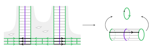
Figure 1. An admissible surface after the transversality procedure. The gray regions map into $C$.

Finally, we define $S_{0}=S_{\partial}\cup S_{b}$ and $S_{1}=S-\operatorname{int}(S_{0})$. Observe that $f$ maps $\partial S_{1}$ into $C$.

The boundary $\partial S_{0}$ decomposes into two subsets: $\partial S$, called the outer boundary, and components in the interior of $S$, called the inner boundary, denoted $\partial^{-}S_{0}$. Note that $\partial^{-}S_{0}=S_{0}\cap S_{1}=\partial S_{1}$. In particular, components of the inner boundary map by $f$ to loops in $X$ representing conjugacy classes of powers of $a$.

Remark 3.1.

Call a loop $f\colon\thinspace S^{1}\to X$ regular if $S^{1}$ can be decomposed into vertices and edges such that the restriction of $f$ to each edge factors through the characteristic map of a $1$–cell of $X$. Note that a regular map is completely described (up to reparametrization) by a cyclic word in the generators $a^{\pm 1}$, $t^{\pm 1}$ representing the conjugacy class of $f$ in $\pi_{1}(X)$.

If a singular surface $S\to X$ has the property that its restriction to each boundary component is regular, then the transversality procedure described above can be performed rel boundary, so that the cyclic orderings of oriented $a$– and $t$–squares in $S_{\partial}$ agree with the cyclic boundary words one started with.

Recall that $\operatorname{scl}(g)$ is the infimum of $\frac{-\chi(S)}{2n(S)}$ over all positive admissible surfaces. We will show how to compute $\operatorname{scl}(g)$ using the decomposition described above.

Choose a cyclically reduced word $w$ representing the conjugacy class of $g$. For any positive admissible surface $S$, each boundary component maps by a loop representing a positive power of $g$ in $\pi_{1}(X)$. Modify $f$ by a homotopy to arrange that its boundary maps are regular, with corresponding cyclic words equal to positive powers of $w$. Then perform the transversality procedure given above, keeping the boundary map fixed (cf. Remark 3.1). At this point, the subsurfaces $S_{0}$, $S_{1}$ are defined. Each boundary component is labeled by a positive power of $w$ and these powers add to $n(S)$.

Note that $\chi(S)=\chi(S_{0})+\chi(S_{1})$ since $S_{0}$ and $S_{1}$ meet along circles. Also,

$$\chi(S_{0})\ =\ \frac{-n(S)\left\lvert{g}\right\rvert_{t}}{2},$$

as this is exactly the number of bands in $S_{b}$, each band connecting two instances of $t^{\pm 1}$ in $w^{n(S)}$ and contributing $-1$ to $\chi(S_{0})$. (Note that $\chi(S_{\partial})=0$.) Let $\chi^{+}(S_{1})$ denote the number of disk components in $S_{1}$. We have

$$\chi(S)\ =\ \frac{-n(S)\left\lvert{g}\right\rvert_{t}}{2}+\chi(S_{1})\ \leqslant\ \frac{-n(S)\left\lvert{g}\right\rvert_{t}}{2}+\chi^{+}(S_{1}),$$

and therefore

$$\frac{-\chi(S)}{2n(S)}\ \geqslant\ \frac{\left\lvert{g}\right\rvert_{t}}{4}\ -\ \frac{\chi^{+}(S_{1})}{2n(S)}.$$

From this, we conclude that

$$\operatorname{scl}(g)\ \geqslant\ \frac{\left\lvert{g}\right\rvert_{t}}{4}\ +\ \inf_{S}\frac{-\chi^{+}(S_{1})}{2n(S)},$$ (5)

where the infimum is taken over all positive admissible surfaces. In fact, the reverse of inequality (5) holds as well:

Lemma 3.2.

There is an equality

$$\operatorname{scl}(g)\ =\ \frac{\left\lvert{g}\right\rvert_{t}}{4}\ +\ \inf_{S}\frac{-\chi^{+}(S_{1})}{2n(S)}.$$

Proof.

Given an admissible surface $S\to X$ decomposed as above, let $S^{\prime}$ be the union of $S_{0}$ and the disk components of $S_{1}$. Recall that the components of $\partial S^{\prime}$ in $\partial^{-}S_{0}$ map to loops in $X$ representing conjugacy classes of powers of $a$. Thus Lemma 2.2 and Lemma 2.3 imply

$$\operatorname{scl}(g)\ \leqslant\ \frac{-\chi(S^{\prime})}{2n(S)}+\frac{1}{n(S)}\sum\operatorname{scl}(a^{p_{i}})\ =\ \frac{-\chi(S^{\prime})}{2n(S)}.$$

Since

$$\frac{-\chi(S^{\prime})}{2n(S)}\ =\ \frac{-\chi(S_{0})}{2n(S)}-\frac{\chi^{+}(S_{1})}{2n(S)}\ =\ \frac{\left\lvert{g}\right\rvert_{t}}{4}-\frac{\chi^{+}(S_{1})}{2n(S)}$$

and $S$ was arbitrary, the reverse of inequality (5) holds, as desired. ∎

Lemma 3.3.

If $S$ is an extremal surface for $g$, then $S_{1}$ consists only of disks and annuli.

Proof.

Let $S_{2}$ be the union of the components of $S_{1}$ that have nonnegative Euler characteristic, and let $S_{3}$ be the union of the components of $S_{1}$ that have negative Euler characteristic. Then $S_{2}$ consists only of disks and annuli and $\chi(S_{2})=\chi^{+}(S_{1})$. If $S$ is extremal, we must have

$$\operatorname{scl}(g)\ =\ \frac{-\chi(S)}{2n(S)}\ =\ \frac{\left\lvert{g}\right\rvert_{t}}{4}-\frac{\chi(S_{2})}{2n(S)}-\frac{\chi(S_{3})}{2n(S)}\ =\ \frac{\left\lvert{g}\right\rvert_{t}}{4}-\frac{\chi^{+}(S_{1})}{2n(S)}-\frac{\chi(S_{3})}{2n(S)}.$$

Comparing with Lemma 3.2, this means $\chi(S_{3})\geqslant 0$, meaning that $S_{3}$ must be empty. Thus $S_{1}$ consists only of disks and annuli. ∎

The weighted turn graph

As in [4], we use a graph to keep track of the combinatorics of the inner boundary $\partial^{-}S_{0}$.

Consider a cyclically reduced word $w$ as in (4). A turn in $w$ is a subword of the form $a^{k}$ between two occurrences of $t^{\pm 1}$ considered as a cyclic word. The turns are indexed by the numbers $i=1,\ldots,n$; the $i^{\rm th}$ turn is labeled by the subword $t^{\epsilon_{i}}a^{k_{i}}t^{\epsilon_{i+1}}$. A turn labeled $ta^{k}t^{-1}$ is of type m; a turn labeled $t^{-1}a^{k}t$ is of type $\ell$; all other turns are of mixed type.

The weighted turn graph $\Gamma(w)$ is a directed graph with integer weights assigned to each vertex. The vertices correspond to the turns of $w$ and the weight associated to the $i^{\rm th}$ turn is $k_{i}$. There is a directed edge from turn $i$ to turn $j$ whenever $-\epsilon_{i}=\epsilon_{j+1}$. In other words, if the label of a turn begins with $t^{\pm 1}$, then there is a directed edge from this turn to every other turn whose label ends with $t^{\mp 1}$. The vertices of $\Gamma(w)$ are partitioned into four subsets where the presence of a directed edge between two vertices depends only on which subsets the vertices lie in. Figure 2 shows the turn graph in schematic form.

Figure 2. A schematic picture of the turn graph $\Gamma(w)$.

The edges of the turn graph come in dual pairs: if $e\in\Gamma(w)$ is an edge from turn $i$ to turn $j$, then one verifies easily that there is also an edge $\bar{e}$ from turn $j+1$ to turn $i-1$, and moreover $\bar{\bar{e}}=e$. See Figure 3.

Figure 3. Dual edge pairs in $w$. Whenever there is an edge from turn $i$ to turn $j$, there must also be an edge from turn $j+1$ to turn $i-1$. The labels of these turns share occurrences of $t^{\pm 1}$ with the labels of the original two turns.

A directed circuit in $\Gamma(w)$ is of type m or type $\ell$ if every vertex it visits corresponds to a turn of type $m$ or of type $\ell$, respectively. Otherwise, the circuit is of mixed type. The weight $\omega(\gamma)$ of a directed circuit $\gamma$ is the sum of the weights of the vertices it visits (counted with multiplicity). Given a directed circuit $\gamma$, define

$$\mu(\gamma)\ =\ \left\{\begin{array}[]{ll}m&\text{ if $\gamma$ is of type $m$}\\ \ell&\text{ if $\gamma$ is of type $\ell$}\\ \gcd(m,\ell)&\text{ otherwise.}\end{array}\right.$$

A directed circuit $\gamma$ is a potential disk if $\omega(\gamma)\equiv 0\mod\mu(\gamma)$.

Turn circuits

Let $S\to X$ be a positive admissible surface whose boundary map is regular and labeled by $w^{n(S)}$. Decomposing $S$ as $S_{0}\cup S_{1}$, each inner boundary component of $S_{0}$ can be described as follows. Traversing the curve in the positively oriented direction, one alternately follows the boundary arcs (or sides) of bands in $S_{b}$ and visits turns of $w$ along $S_{\partial}$; such a visit consists in traversing the inner edges of some $a$–squares before proceeding up along another side of a band (cf. Figure 1). If the side of the band leads from turn $i$ to turn $j$, then $(t^{\epsilon_{i}})^{-1}=t^{\epsilon_{j}}$ and therefore there is an edge in $\Gamma(w)$ from turn $i$ to turn $j$. In this way, $\partial^{-}S_{0}$ gives rise to a finite collection (possibly with repetitions) of directed circuits in $\Gamma(w)$, called the turn circuits for $S_{0}$.

Since $\partial S$ is labeled by $w^{n(S)}$, there are $n(S)$ occurrences of each turn on $\partial S$. The turn circuits do not contain the information of which particular instances of turns are joined bands, nor do they record how many times the band corresponding to a given edge in the circuit wraps around the annulus $X-C$.

Remark 3.4.

Given two cyclically reduced words $w,w^{\prime}$ representing the same conjugacy class in $BS(m,\ell)$, there is an isomorphism $\Gamma(w)\to\Gamma(w^{\prime})$ of the underlying directed graph structure that respects vertex type and edge duality but not necessarily the vertex weights. However, a directed circuit is a potential disk with one sets of weights if and only if it is a potential disk with the other set. The difference in weights of a type $m$ vertex is a multiple of $m$, the difference in weights of a type $\ell$ vertex is a multiple of $\ell$, and the difference in weights of mixed type vertex is a multiple of $\gcd(m,\ell)$. See Remark 2.6.

In what follows, only the property of being a potential disk is used and therefore this ambiguity in the weighed turn graph associated to a conjugacy class is not an issue.

Lemma 3.5.

Suppose $\gamma$ is a turn circuit for $S_{0}$ that corresponds to an inner boundary component in $\partial^{-}S_{0}$ that bounds a disk in $S_{1}$. Then $\gamma$ is a potential disk.

Proof.

For any band in $S_{b}$, the core arc (a component of $N_{b}$) maps to $C^{\prime}$ as a loop of some degree $d$. The two sides then map to $C$ as loops of degrees $dm$ and $d\ell$ respectively.

If $\iota$ is the side of a band that leads from a turn labeled $ta^{k}t^{*}$ to a turn labeled $t^{*}a^{k^{\prime}}t^{-1}$ then the map $\iota\to C$ has degree a multiple of $m$. Likewise if $\iota$ leads from a turn labeled $t^{-1}a^{k}t^{*}$ to a turn labeled $t^{*}a^{k^{\prime}}t$ then $\iota$ maps to $C$ with degree a multiple of $\ell$.

Therefore the total degree of an inner boundary component corresponding to a turn circuit $\gamma$ is $\omega(\gamma)+dm+d^{\prime}\ell$ for some integers $d,d^{\prime}$. If $\gamma$ is of type $m$ then $d^{\prime}=0$. Likewise, if $\gamma$ is of type $\ell$ then $d=0$.

If the boundary component actually bounds a disk in $S_{1}$ then this total degree is $0$. Hence $\omega(\gamma)\equiv 0\mod\mu(\gamma)$ and therefore $\gamma$ is a potential disk. ∎

4. Linear optimization

We would like to convert the optimization problem in Lemma 3.2 to a problem of optimizing a certain linear functional on a vector space whose coordinates correspond to possible potential disks, subject to certain linear constraints. Here the functional would count the number of potential disks, and the constraints would arise from the pairing of edges in the turn graph. The objective would then be to compute stable commutator length using classical linear programming.

The main difficulty in such an approach is arranging that the optimization takes place over a finite dimensional object. In this section, we show how to convert an admissible surface to a vector in a finite dimensional vector space in such a way that the number of disk components of $S_{1}$ is less than the value of an appropriate linear functional. We thus obtain computable, rational lower bounds for the stable commutator length of elements of Baumslag–Solitar groups (Theorem 4.3). In Section 5, we will show that these bounds are sharp for a certain class of elements.

We construct the finite dimensional vector space as follows. Let $w$ be a conjugate of $g$ of the form given in Remark 2.6. Let $M=\max\{\left\lvert{m}\right\rvert,\left\lvert{\ell}\right\rvert\}$. We consider two sets of directed circuits in $\Gamma(w)$:

• $\mathfrak{X}$: the set of potential disks that are a sum of not more than $M$ embedded circuits, and

• $\mathfrak{Y}$: the set of all embedded circuits.

Note that both $\mathfrak{X}$ and $\mathfrak{Y}$ are finite sets and that they may have some circuits in common. Enumerate these sets as $\mathfrak{X}=\{\alpha_{1},\ldots,\alpha_{p}\}$ and $\mathfrak{Y}=\{\beta_{1},\ldots,\beta_{q}\}$. Let ${\mathbb{X}}$ be a $p$–dimensional real vector space with basis $\{\mathbf{x}_{1},\ldots,\mathbf{x}_{p}\}$, and let ${\mathbb{Y}}$ be a $q$–dimensional real vector space with basis $\{\mathbf{y}_{1},\ldots,\mathbf{y}_{q}\}$. Equip both ${\mathbb{X}}$ and ${\mathbb{Y}}$ with an inner product that makes the respective bases orthonormal. By Remark 3.4, the vector spaces ${\mathbb{X}}$ and ${\mathbb{Y}}$ depend only on the conjugacy class in $BS(m,\ell)$ represented by $w$. Abusing notation, we let $\{\mathbf{x}_{1},\ldots,\mathbf{x}_{p},\mathbf{y}_{1},\ldots,\mathbf{y}_{q}\}$ denote the corresponding orthonormal basis of ${\mathbb{X}}\oplus{\mathbb{Y}}$. This is the vector space with which we will work.

The linear functional on the vector space ${\mathbb{X}}\oplus{\mathbb{Y}}$ whose values will be compared with the number of disk components of $S_{1}$ is the functional that is the sum of the coordinates corresponding to ${\mathbb{X}}$, i.e. the functional that takes in $\mathbf{u}\in{\mathbb{X}}\oplus{\mathbb{Y}}$ and gives out $\left\lvert{\mathbf{u}}\right\rvert_{\mathbb{X}}:=\sum_{i=1}^{p}\mathbf{u}\cdot\mathbf{x}_{i}$. One thinks of this functional as counting the number of potential disks.

There are additional linear functionals on ${\mathbb{X}}\oplus{\mathbb{Y}}$ that count the number of times turn circuits in a given collection visit a specific vertex or edge. For each vertex $v\in\Gamma(w)$, define $F_{v}\colon\thinspace{\mathbb{X}}\oplus{\mathbb{Y}}\to{\mathbb{R}}$ by letting $F_{v}(\mathbf{x}_{i})$ be the number of times $\alpha_{i}$ visits $v$, letting $F_{v}(\mathbf{y}_{i})$ be the number of times $\beta_{i}$ visits $v$, and extending by linearity. For each edge $e\subset\Gamma(w)$, define $F_{e}\colon\thinspace{\mathbb{X}}\oplus{\mathbb{Y}}\to{\mathbb{R}}$ by letting $F_{e}(\mathbf{x}_{i})$ be the number of times $\alpha_{i}$ traverses $e$, letting $F_{v}(\mathbf{y}_{i})$ be the number of times $\beta_{i}$ traverses $e$, and extending by linearity.

One thinks of the next lemma as saying that, if a collection of turn circuits traverses each edge the same number of times as its dual edge, then this collection of turn circuits visits each vertex the same number of times.

Lemma 4.1.

If $F_{e}(\mathbf{u})=F_{\bar{e}}(\mathbf{u})$ for each dual edge pair $e,\bar{e}$ of $\Gamma(w)$, then $F_{v}(\mathbf{u})=F_{v^{\prime}}(\mathbf{u})$ for any vertices $v,v^{\prime}\in\Gamma(w)$.

Proof.

For a vertex $v\in\Gamma(w)$, let $E^{+}(v)$ be the set of directed edges that are outgoing from $v$ and let $E^{-}(v)$ be the set directed edges that are incoming to $v$. Then

$$F_{v}(\mathbf{u})=\sum_{e\in E^{+}(v)}F_{e}(\mathbf{u})=\sum_{e\in E^{-}(v)}F_{e}(\mathbf{u}).$$

First suppose that $v$ corresponds to turn $i$ and $v^{\prime}$ corresponds to turn $i-1$. Then edge duality gives a pairing between edges in $E^{+}(v)$ and edges in $E^{-}(v^{\prime})$. Since $F_{e}(\mathbf{u})=F_{\bar{e}}(\mathbf{u})$ for every dual edge pair $e,\bar{e}$, we have that

$$F_{v}(\mathbf{u})=\sum_{e\in E^{+}(v)}F_{e}(\mathbf{u})=\sum_{e\in E^{+}(v)}F_{\bar{e}}(\mathbf{u})=\sum_{e\in E^{-}(v^{\prime})}F_{e}(\mathbf{u})=F_{v^{\prime}}(\mathbf{u}).$$

Letting $i$ vary, we obtain a similar statement for all pairs of vertices corresponding to adjacent turns. It follows that $F_{v}(\mathbf{u})=F_{v^{\prime}}(\mathbf{u})$ for any vertices $v,v^{\prime}\in\Gamma(w)$. ∎

Let $C\subset{\mathbb{X}}\oplus{\mathbb{Y}}$ be the cone of non-negative vectors $\mathbf{u}$ such that $F_{e}(\mathbf{u})=F_{\bar{e}}(\mathbf{u})$ for every dual edge pair $e,\bar{e}$ of $\Gamma(w)$. In light of the lemma, we denote by $F\colon\thinspace C\to{\mathbb{R}}$ the function $F_{v}\big{|}_{C}$ for any vertex $v\in\Gamma(w)$.

The following proposition shows how to convert an admissible surface into a vector $\mathbf{u}\in C$ in such a way that $\left\lvert{\mathbf{u}}\right\rvert_{\mathbb{X}}$ is at least the number of disk components of $S_{1}$.

Proposition 4.2.

Given an admissible surface $S\to X$, there is a vector $\mathbf{u}\in C$ such that

$$\frac{\left\lvert{\mathbf{u}}\right\rvert_{\mathbb{X}}}{F(\mathbf{u})}\geqslant\frac{\chi^{+}(S_{1})}{n(S)}.$$ (6)

Proof.

Suppose the surface $S$ has been decomposed as $S_{0}\cup S_{1}$ as described in Section 3, and consider the collection of turn circuits for $S_{0}$. Let $\gamma$ be one of the turn circuits in this collection. As a cycle we can decompose $\gamma$ as a sum of embedded circuits, i.e.  $\gamma=\beta_{i_{1}}+\cdots+\beta_{i_{k}}$. This decomposition may not be unique, but we only need its existence.

For each turn circuit $\gamma$, we will construct a corresponding vector $\mathbf{u}(\gamma)$, depending on this decomposition and on whether the corresponding boundary component of $\partial^{-}S_{0}$ bounds a disk in $S_{1}$. If the corresponding inner boundary component of $\partial^{-}S_{0}$ does not bound a disk in $S_{1}$, we define

$$\mathbf{u}(\gamma)=\sum_{j=1}^{k}\mathbf{y}_{i_{j}}.$$

Otherwise, the corresponding inner boundary component of $\partial^{-}S_{0}$ does bound a disk in $S_{1}$, in which case Lemma 3.5 implies that $\gamma$ is a potential disk. If $k\leqslant M$, then $\gamma\in\mathfrak{X}$; say $\gamma=\alpha_{i}$. In this case we define $\mathbf{u}(\gamma)=\mathbf{x}_{i}$. Otherwise, if $k>M$, we proceed as follows. For each $\beta_{i_{j}}$, let $\mu(\beta_{i_{j}})\beta_{i_{j}}$ denote the sum of $\mu(\beta_{i_{j}})$ copies of $\beta_{i_{j}}$. Notice that $\mu(\beta_{i_{j}})\beta_{i_{j}}$ is a potential disk that is not the sum of more than $M$ embedded circuits. Hence $\mu(\beta_{i_{j}})\beta_{i_{j}}\in\mathfrak{X}$, so $\mu(\beta_{i_{j}})\beta_{i_{j}}=\alpha_{i^{\prime}_{j}}$ for some $i^{\prime}_{j}\in\{1,\ldots,p\}$. In this case we define

$$\mathbf{u}(\gamma)=\sum_{j=1}^{k}\frac{1}{\mu(\beta_{i_{j}})}\mathbf{x}_{i^{\prime}_{j}}.$$

The vector we will consider is $\mathbf{u}=\sum_{\gamma}\mathbf{u}(\gamma)$, where this sum is taken over all $\gamma$ in the collection of turn circuits for $S_{0}$ (with multiplicity). Establishing the following three claims will complete the proof of the proposition.

1. $\mathbf{u}\in C$,

2. $F(\mathbf{u})=n(S)$, and

3. $|\mathbf{u}|_{\mathbb{X}}\geqslant\chi^{+}(S_{1})$.

(i): The vector $\mathbf{u}(\gamma)$ was constructed so that $F_{e}(\mathbf{u}(\gamma))$ counts the number of times the turn circuit $\gamma$ traverses the edge $e$. Thus $F_{e}(\mathbf{u})$ records the number of times turn circuits for $S_{0}$ traverse $e$. Every time an edge $e$ is traversed by a turn circuit for $S_{0}$, there is a band in $S_{b}$ one side of which represents $e$. The other side of this band represents $\bar{e}$, so therefore we have that $F_{e}(\mathbf{u})=F_{\bar{e}}(\mathbf{u})$ for all edges $e$. Thus $\mathbf{u}\in C$.

(ii): The vector $\mathbf{u}(\gamma)$ was also constructed so that $F_{v}(\mathbf{u}(\gamma))$ counts the number of times the turn circuit $\gamma$ visits the vertex $v$. Therefore $F(\mathbf{u})$ records the number of times turn circuits for $S_{0}$ visit any given vertex. As each turn occurs once in $w$, each vertex must be visited exactly $n(S)$ times. Thus $F(\mathbf{u})=n(S)$.

(iii): Let $\gamma$ be a turn circuit for $S_{0}$, and suppose the corresponding inner boundary component of $S_{0}$ bounds a disk in $S_{1}$. Decompose $\gamma$ as a sum $\beta_{i_{1}}+\cdots+\beta_{i_{k}}$ of embedded circuits as above. If $k\leqslant M$, then $\mathbf{u}(\gamma)=\mathbf{x}_{i}$ for some $i\in\{1,\ldots,p\}$, and thus $\left\lvert{\mathbf{u}(\gamma)}\right\rvert_{\mathbb{X}}=1$. Otherwise, we have

$$\left\lvert{\mathbf{u}(\gamma)}\right\rvert_{\mathbb{X}}=\sum_{j=1}^{k}\frac{1}{\mu(\beta_{i_{j}})}\geqslant\sum_{j=1}^{k}\frac{1}{M}=\frac{k}{M}\geqslant 1.$$

In either case, $\left\lvert{\mathbf{u}(\gamma)}\right\rvert_{\mathbb{X}}\geqslant 1$. As $\left\lvert{{\mathchoice{\mkern 1.0mu\mbox{\raise 2.2pt\hbox{$\centerdot$}}\mkern 1.0mu}{\mkern 1.0mu\mbox{\raise 2.2pt\hbox{$\centerdot$}}\mkern 1.0mu}{\mkern 1.5mu\centerdot\mkern 1.5mu}{\mkern 1.5mu\centerdot\mkern 1.5mu}}}\right\rvert_{\mathbb{X}}$ is a linear functional, we thus have that $\left\lvert{\mathbf{u}}\right\rvert_{\mathbb{X}}\geqslant\chi^{+}(S_{1})$. ∎

Theorem 4.3.

Let $g\in BS(m,\ell)$, $m\neq\ell$, be of $t$–exponent zero. Then there is a computable, finite sided, rational polyhedron $P\subset{\mathbb{X}}\oplus{\mathbb{Y}}$ such that

$$\operatorname{scl}(g)\geqslant\frac{|g|_{t}}{4}-\frac{1}{2}\max\left\{\left\lvert{\mathbf{u}}\right\rvert_{\mathbb{X}}\mid\mathbf{u}\text{ is a vertex of }P\right\}.$$ (7)

Proof.

Let $P=F^{-1}(1)$. If $V$ is the number of vertices of $\Gamma(w)$, we can extend $F$ to a linear functional $\widetilde{F}\colon\thinspace{\mathbb{X}}\oplus{\mathbb{Y}}\to{\mathbb{R}}$ by setting $\widetilde{F}(\mathbf{u})=\frac{1}{V}\sum_{v}F_{v}(\mathbf{u})$, where the sum is taken over all vertices of $\Gamma(w)$. The linear functional $\widetilde{F}$ is positive on all basis vectors of ${\mathbb{X}}\oplus{\mathbb{Y}}$, and hence a level set of $\widetilde{F}$ intersects the positive cone in a compact set. Clearly $P=C\cap\widetilde{F}^{-1}(1)$. Thus $P$ is a finite sided, rational, compact polyhedron.

By Lemma 3.2, Proposition 4.2, and the linearity of $\left\lvert{{\mathchoice{\mkern 1.0mu\mbox{\raise 2.2pt\hbox{$\centerdot$}}\mkern 1.0mu}{\mkern 1.0mu\mbox{\raise 2.2pt\hbox{$\centerdot$}}\mkern 1.0mu}{\mkern 1.5mu\centerdot\mkern 1.5mu}{\mkern 1.5mu\centerdot\mkern 1.5mu}}}\right\rvert_{\mathbb{X}}$ and $F$, we have that

$$\operatorname{scl}(g) =\ \frac{\left\lvert{g}\right\rvert_{t}}{4}\ +\ \frac{1}{2}\inf_{S}\frac{-\chi^{+}(S_{1})}{n(S)}$$

$$=\ \frac{\left\lvert{g}\right\rvert_{t}}{4}\ -\ \frac{1}{2}\sup_{S}\frac{\chi^{+}(S_{1})}{n(S)}$$

$$\geqslant\ \frac{\left\lvert{g}\right\rvert_{t}}{4}\ -\ \frac{1}{2}\sup_{\mathbf{u}\in C}\frac{\left\lvert{\mathbf{u}}\right\rvert_{\mathbb{X}}}{F(\mathbf{u})}$$

$$\geqslant\ \frac{\left\lvert{g}\right\rvert_{t}}{4}\ -\ \frac{1}{2}\sup_{\mathbf{u}\in P}\left\lvert{\mathbf{u}}\right\rvert_{\mathbb{X}}.$$

As $P$ is a finite sided, compact polyhedron and $\left\lvert{{\mathchoice{\mkern 1.0mu\mbox{\raise 2.2pt\hbox{$\centerdot$}}\mkern 1.0mu}{\mkern 1.0mu\mbox{\raise 2.2pt\hbox{$\centerdot$}}\mkern 1.0mu}{\mkern 1.5mu\centerdot\mkern 1.5mu}{\mkern 1.5mu\centerdot\mkern 1.5mu}}}\right\rvert_{\mathbb{X}}$ is a linear functional, the supremum is realized at one of the vertices of $P$. This gives (7). ∎

Remark 4.4.

If $\mathbf{u}$ is a vertex of $P$ that maximizes $\left\lvert{\mathbf{u}}\right\rvert_{\mathbb{X}}$ in $P$, then $\mathbf{u}\cdot\mathbf{y}_{i}=0$ for all $i\in\{1,\ldots,q\}$. Indeed, suppose not and let $\beta_{i}\in\mathfrak{Y}$ be such that $\mathbf{u}\cdot\mathbf{y}_{i}=c>0$. Then there is some $\alpha_{i^{\prime}}\in\mathfrak{X}$ such that $\mu(\beta_{i})\beta_{i}=\alpha_{i^{\prime}}$. One then observes that $\mathbf{u}^{\prime}=\mathbf{u}-c\mathbf{y}_{i}+\frac{c}{\mu(\beta_{i})}\mathbf{x}_{i^{\prime}}\in P$ and $\left\lvert{\mathbf{u}^{\prime}}\right\rvert_{\mathbb{X}}>\left\lvert{\mathbf{u}}\right\rvert_{\mathbb{X}}$.

The linear programming problem described in this section has been implemented using Sage [19] and is available from the first author’s webpage. The number of embedded circuits in $\Gamma(w)$ is on the order of $\left\lvert{w}\right\rvert_{t}!$ and so the algorithm is only practical for elements with small $t$–length.

5. Elements of alternating $t$–shape

The bounds given in Theorem 4.3 are not always sharp, as we will point out in Remark 5.4. However, we show in Theorem 5.2 that these bounds are sharp for a class of elements that have what we call alternating $t$–shape. We thus show that stable commutator length is computable and rational for such elements. We also characterize which elements of alternating $t$–shape admit extremal surfaces (Theorem 5.7).

Definition 5.1.

We say that an element $g\in BS(m,\ell)$ has alternating $t$–shape if it has a conjugate of the form given in Remark 2.6 where $n$ is even and $\epsilon_{i}=(-1)^{i-1}$.

In this section, we restrict attention to elements of alternating $t$–shape and express this conjugate as

$$w=\prod_{k=1}^{r}ta^{i_{k}}t^{-1}a^{j_{k}}.$$ (8)

Note that if $g$ has alternating $t$–shape then it has $t$–exponent zero. Hence stable commutator length is finite for elements of alternating $t$–shape.

Constructing surfaces

Let $P$ be as in the proof of Theorem 4.3, and let

$$L(g)=\frac{|g|_{t}}{4}-\frac{1}{2}\max\left\{\left\lvert{\mathbf{u}}\right\rvert_{\mathbb{X}}\mid\mathbf{u}\text{ is a vertex of }P\right\}.$$

To show that the lower bound $L(g)$ on stable commutator length is sharp, we would like to find a surface $S$ that gives the same upper bound on stable commutator length. Specifically, given a vertex $\mathbf{u}\in P$, we want to construct a corresponding surface $S=S_{0}\cup S_{1}$ of the type discussed in Section 3, where $\partial S$ maps to loops representing conjugacy classes of powers of $g$ and $\partial S_{1}$ maps to loops representing conjugacy classes of powers of $a$. Such a surface $S_{0}$ can be built (in fact, many such surfaces can be built); the construction is given in the proof of Theorem 5.2. The difficulty is arranging $S_{0}$ so that its inner boundary components can be efficiently capped off by $S_{1}$.

If the degree of each inner boundary component of $S_{0}$ were zero, we could take each component of $S_{1}$ to be a disk. In this case, we would have $\left\lvert{\mathbf{u}}\right\rvert_{\mathbb{X}}=\chi^{+}(S_{1})=\chi(S_{1})$ and

$$\operatorname{scl}(g)\leqslant\frac{-\chi(S)}{2n(S)}=\frac{\left\lvert{g}\right\rvert_{t}}{4}-\frac{\chi(S_{1})}{2n(S)}=L(g)\leqslant\operatorname{scl}(g).$$

This would mean the bound in Theorem 4.3 is sharp and the surface $S$ is extremal.

It may not be the case that all inner boundary components of $S_{0}$ can be made to have degree zero. Nevertheless, when $g$ has alternating $t$–shape, we can control the number of inner boundary components of $S_{0}$ that have nonzero degree in such a way as to show that there are surfaces $S$ for which $\frac{-\chi(S)}{2n(S)}$ is arbitrarily close to $L(g)$. The details are given in the proof of Theorem 5.2. In this way, we establish that the lower bound given in Theorem 4.3 is sharp for elements of alternating $t$–shape.

Theorem 5.2.

Let $g\in BS(m,\ell)$, $m\neq\ell$, have alternating $t$–shape. Then

$$\operatorname{scl}(g)=L(g).$$

Proof.

We will show that $\operatorname{scl}(g)<L(g)+\epsilon$ for all $\epsilon>0$. Note that, since $g$ is of alternating $t$–shape, all circuits in the turn graph are either of type $m$ or of type $\ell$, not of mixed type. Let $\mathbf{u}$ be a vertex of $P$ on which $\left\lvert{{\mathchoice{\mkern 1.0mu\mbox{\raise 2.2pt\hbox{$\centerdot$}}\mkern 1.0mu}{\mkern 1.0mu\mbox{\raise 2.2pt\hbox{$\centerdot$}}\mkern 1.0mu}{\mkern 1.5mu\centerdot\mkern 1.5mu}{\mkern 1.5mu\centerdot\mkern 1.5mu}}}\right\rvert_{\mathbb{X}}$ is maximal. Since $P$ is a rational polyhedron on which all coordinates are nonnegative, all coordinates of $\mathbf{u}$ are nonnegative rational numbers. By Remark 4.4, $\mathbf{u}$ has nonzero entries only in coordinates corresponding to ${\mathbb{X}}$. Let $K$ denote the number of edges in the turn graph. Let $N$ be an integer such that each coordinate of $N\mathbf{u}$ is a nonnegative integer and such that $N>K/2\epsilon$ (so that $K/2N<\epsilon$).

Each coordinate $\mathbf{x}_{i}$ of ${\mathbb{X}}$ represents a directed circuit $\gamma$ in the turn graph. For each such directed circuit $\gamma$ of length $n$, we consider a $2n$–gon with alternate sides labeled by the powers of $a$ corresponding to the vertices of the turn graph through which $\gamma$ passes and alternate sides labeled by the intervening edges of the turn graph traversed by $\gamma$. See Figure 4.

Figure 4. A sample polygon corresponding to a circuit $\gamma$ of length $2$.

For each $i$ we take $N\mathbf{u}\cdot\mathbf{x}_{i}$ copies of the polygon corresponding to $\mathbf{x}_{i}$, thus obtaining a collection $Q_{1},\dotsc,Q_{s}$ of polygons. Since $F_{e}(N\mathbf{u})=F_{\bar{e}}(N\mathbf{u})$, there exists a pairing of the edges of these polygons corresponding to edges of the turn graph such that each edge labeled by $e$ on a polygon $Q_{i}$ is paired with an edge labeled by $\bar{e}$ on a polygon $Q_{j}$. Let $\Delta$ be the graph dual to this pairing, i.e. the graph with a vertex for each polygon $Q_{i}$ and an edge between the vertex corresponding to $Q_{i}$ and the vertex corresponding to $Q_{j}$ for each edge of $Q_{i}$ that is paired with an edge from $Q_{j}$. The graph $\Delta$ may have many components. However, we can adjust the pairings of edges of polygons to obtain some control over the number of components of $\Delta$. Suppose $Q_{i_{1}}$ and $Q_{i_{2}}$ are polygons where an edge labeled $e$ of $Q_{i_{1}}$ has been paired with an edge labeled $\bar{e}$ of $Q_{i_{2}}$, and suppose $Q_{j_{1}}$ and $Q_{j_{2}}$ are polygons in another component of $\Delta$ where an edge labeled $e$ of $Q_{j_{1}}$ has been paired with an edge labeled $\bar{e}$ of $Q_{j_{2}}$. Then we can modify the pairing of edges to instead pair the edge labeled $e$ of $Q_{i_{1}}$ with the edge labeled $\bar{e}$ of $Q_{j_{2}}$ and the edge labeled $e$ of $Q_{j_{1}}$ with the edge labeled $\bar{e}$ of $Q_{i_{2}}$. The graph $\Delta$ corresponding to this pairing will have one fewer component than the graph corresponding to the original pairing. See Figure 5. Such a modification can be done any time there are two components of $\Delta$ on which edges with the same labels have been paired. Therefore, we can arrange that the number of components of $\Delta$ is no more than $K$, the number of edges in the turn graph. Note that $\Delta$ is naturally a bipartite graph, with vertices partitioned into those corresponding to turn circuits of type $m$ (“type $m$ vertices”) and those corresponding to turn circuits of type $\ell$ (“type $\ell$ vertices”).

Figure 5. Modifying the edges in $\Delta$ to reduce the number of components.

If a vertex $v\in\Delta$ corresponds to a turn circuit $\gamma$, we define the weight of $v$ to be $\omega(v):=\omega(\gamma)$. If $v$ is a type $m$ vertex we have that $m\mid\omega(v)$, and if $v$ is a type $\ell$ vertex we have that $\ell\mid\omega(v)$. We wish to assign an integer $\omega(e)$ to each edge $e\in\Delta$ such that, whenever $v$ is of type $m$, we have

$$\omega(v)-m\sum_{e\ni v}\omega(e)=0,$$ (9)

and, whenever $v$ is of type $\ell$, we have

$$\omega(v)+\ell\sum_{e\ni v}\omega(e)=0.$$ (10)

On each connected component of $\Delta$, proceed as follows. For each type $m$ vertex $v$, choose a preferred edge $e_{v}$ emanating from $v$. For each $v$, set $\omega(e_{v})=\omega(v)/m$, and let $\omega(e)=0$ for all other edges $e$. This makes (9) hold for all vertices of type $m$. Now choose a preferred type $\ell$ vertex $v_{0}$. For another type $\ell$ vertex $v_{1}$, let

$$\Omega=\frac{\omega(v_{1})}{\ell}+\sum_{e\ni v_{1}}\omega(e).$$

Choose a path $e_{1},\dotsc,e_{k}$ connecting $v_{1}$ to $v_{0}$, and modify the weights $\omega(e_{i})$ by decreasing $\omega(e_{i})$ by $\Omega$ whenever $i$ is odd and increasing $\omega(e_{i})$ by $\Omega$ whenever $i$ is even. For all vertices other than $v_{1}$ and $v_{0}$, this does not change the quantities in (9) and (10). Moreover, this causes (10) to now be true for $v_{1}$. Fixing $v_{0}$ and letting $v_{1}$ vary over all type $\ell$ vertices other than $v_{0}$, we obtain edge weights $\omega(e)$ such that (9) and (10) are true for all vertices on this component of $\Delta$ except for $v_{0}$. Thus we obtain edge weights $\omega(e)$ such that (9) and (10) are true for all vertices except for one vertex in each component of $\Delta$.

We now proceed to build a surface. Rather than building a surface from the polygons $Q_{i}$, we use them to build a band surface $S_{0}$, then attempt to fill various components of $\partial S_{0}$ with disks. For each pairing of an edge of $Q_{i}$ with an edge of $Q_{j}$, insert a rectangle with sides labeled by $t$, $a^{m\omega(e)}$, $t^{-1}$, and $a^{-\ell\omega(e)}$, where $\omega(e)$ is the weight assigned to the corresponding edge of $\Delta$. See Figure 6.

Figure 6. Using the polygons $Q_{i}$ to build a band surface $S_{0}$. The surface $S_{0}$ is shaded above.

Note that the edges of these rectangles labeled $t$ and $t^{-1}$, together with the edges of the polygons labeled by powers of $a$, form paths that would map to the $1$–skeleton of $X$. By construction, these paths correspond exactly to powers of $w$. To each of these paths, attach an annulus $S^{1}\times[0,1]$ labeled on both sides by this power of $w$. The rectangles and annuli together form $S_{0}$, shown in Figure 6. Note that each rectangle maps naturally to the $2$–cell of $X$ with degree $\omega(e)$. The annuli map to the $1$–skeleton of $X$, as indicated by the labels, with the map factoring through the projection $S^{1}\times[0,1]\to S^{1}$.

As in Section 3, we refer to the boundary components of $S_{0}$ that map to a power of $w$ as outer boundary components and to those corresponding to a polygon $Q_{i}$ as inner boundary components. Each of the inner boundary components of $S_{0}$ maps to a power of $a$; let $d$ be the number of components of the inner boundary for which this power is zero. The powers of $a$ on the inner boundary components are exactly the quantities on the left-hand sides of (9) and (10). The weights $\omega(e)$ have been chosen so that these quantities are zero for all but $K$ components of the inner boundary, so therefore $d\geqslant s-K$. Fill these $d$ components of the inner boundary with disks, and call the resulting surface $S$.

Each inner boundary component of $S$ maps to a power of $a$, and Lemma 2.3 says that $\operatorname{scl}(a)=0$. Therefore, applying Lemma 2.2, we have that

$$\operatorname{scl}(g) \leqslant\frac{-\chi(S)}{2n(S)}$$

$$=\frac{\left\lvert{g}\right\rvert_{t}}{4}-\frac{d}{2N}$$

$$\leqslant\frac{\left\lvert{g}\right\rvert_{t}}{4}-\frac{s-K}{2N}$$

$$=\frac{\left\lvert{g}\right\rvert_{t}}{4}-\frac{s}{2N}+\frac{K}{2N}$$

$$<\frac{\left\lvert{g}\right\rvert_{t}}{4}-\frac{1}{2}\max\left\{\left\lvert{\mathbf{u}}\right\rvert_{\mathbb{X}}\mid\mathbf{u}\text{ is a vertex of }P\right\}+\epsilon$$

$$=L(g)+\epsilon.$$

Thus $\operatorname{scl}(g)=L(g)$, as desired. ∎

Corollary 5.3.

If $g\in BS(m,\ell)$, $m\neq\ell$, has alternating $t$–shape, then $\operatorname{scl}(g)$ is rational.

Proof.

Since each vertex $\mathbf{u}$ of $P$ has rational coordinates and $\left\lvert{\mathbf{u}}\right\rvert_{{\mathbb{X}}}$ is the sum of certain of these coordinates, we know that $L(g)$ is rational. Therefore it follows from Theorem 5.2 that $\operatorname{scl}(g)$ is rational. ∎

Remark 5.4.

In general one suspects the inequality in Theorem 4.3 is strict. For example, the function $\left\lvert{\mathbf{u}}\right\rvert_{\mathbb{X}}$ has a unique maximum on the polyhedron $P$ in Theorem 4.3 for the element $a^{2}t^{2}at^{-1}at^{-1}\in BS(2,3)$. When attempting to build a surface from this unique optimal vertex $\mathbf{u}$, it turns out that every component of the dual graph $\Delta$ has a constant proportion of vertices that cannot be filled, regardless of the edge weights.

Therefore, in contrast to Theorem 5.2, where all but at most a constant number of vertices can be filled, there is no sequence of surfaces associated to $\mathbf{u}$ to for which $\frac{\chi^{+}(S)}{n(S)}$ approaches $\left\lvert{\mathbf{u}}\right\rvert_{\mathbb{X}}$.

An explicit formula

When $\left\lvert{g}\right\rvert_{t}=2$ the turn graph consists of two vertices, each adjacent to a one-edge loop. In this case the vector space ${\mathbb{X}}$ is essentially two dimensional and the linear optimization problem can be solved easily by hand, resulting in a formula for stable commutator length for such elements.

This calculation is interesting for two reasons. First, it is rare that one can derive a formula for $\operatorname{scl}$ in non-trivial cases. Second, the minimal value for $\operatorname{scl}$ among all “well-aligned” elements (see Definition 6.8 and Theorem 6.9) is realized by an element of this type.

Proposition 5.5.

In the group $BS(m,\ell)$ with $m\not=\ell$, if $m\nmid i$ and $\ell\nmid j$ then

$$\operatorname{scl}(ta^{i}t^{-1}a^{j})\ =\ \frac{1}{2}\left(1-\frac{\gcd(i,m)}{\left\lvert{m}\right\rvert}-\frac{\gcd(j,\ell)}{\left\lvert{\ell}\right\rvert}\right).$$

The divisibility hypotheses simply mean that the word $ta^{i}t^{-1}a^{j}$ is cyclically reduced (cf. Remark 2.6).

Proof.

The turn graph for the word $ta^{i}t^{-1}a^{j}$ is as shown in Figure 7.

Figure 7. The turn graph for $ta^{i}t^{-1}a^{j}$.

There are two types of potential disks:

1. Circuits of type $m$ that traverse the left loop of the turn graph $p$ times, where $m\mid pi$.

2. Circuits of type $\ell$ that traverse the right loop of the turn graph $q$ times, where $\ell\mid qj$.

Note that the condition $m\mid pi$ is equivalent to $\frac{\left\lvert{m}\right\rvert}{\gcd(i,m)}\mid p$, and the condition $\ell\mid qj$ is equivalent to $\frac{\left\lvert{\ell}\right\rvert}{\gcd(j,\ell)}\mid q$. Suppose $p=\frac{k\left\lvert{m}\right\rvert}{\gcd(i,m)}$, where $p\leqslant\max\{\left\lvert{m}\right\rvert,\left\lvert{\ell}\right\rvert\}$, for some positive integer $k$, and let $\mathbf{x}_{i_{k}}$ be the corresponding basis vector of ${\mathbb{X}}$. We claim that, if $k>1$ and $\mathbf{u}$ is a vertex of $P$ that maximizes $\left\lvert{\mathbf{u}}\right\rvert_{{\mathbb{X}}}$, then $\mathbf{u}\cdot\mathbf{x}_{i_{k}}=0$. Indeed, suppose not, and consider the vector $\mathbf{u}^{\prime}=\mathbf{u}-(\mathbf{u}\cdot\mathbf{x}_{i_{k}})\mathbf{x}_{i_{k}}+k(\mathbf{u}\cdot\mathbf{x}_{i_{k}})\mathbf{x}_{i_{1}}$. Then $F_{e}(\mathbf{u}^{\prime})=F_{e}(\mathbf{u})$ for all $e$ and $F(\mathbf{u}^{\prime})=F(\mathbf{u})=1$, but

$$\left\lvert{\mathbf{u}^{\prime}}\right\rvert_{{\mathbb{X}}}=\left\lvert{\mathbf{u}}\right\rvert_{{\mathbb{X}}}-\mathbf{u}\cdot\mathbf{x}_{i_{k}}+k(\mathbf{u}\cdot\mathbf{x}_{i_{k}})=\left\lvert{\mathbf{u}}\right\rvert_{{\mathbb{X}}}+(k-1)(\mathbf{u}\cdot\mathbf{x}_{i_{k}})>\left\lvert{\mathbf{u}}\right\rvert_{{\mathbb{X}}}.$$

A similar argument applies to coordinates of ${\mathbb{X}}$ corresponding to potential disks of type $\ell$. Thus, if $\mathbf{u}$ is a vertex of $P$ that maximizes $\left\lvert{\mathbf{u}}\right\rvert_{{\mathbb{X}}}$, only two coordinates of $\mathbf{u}$ are nonzero, one corresponding to a potential disk of type $m$ where $p=\frac{\left\lvert{m}\right\rvert}{\gcd(i,m)}$ and the other corresponding to a potential disk of type $\ell$ where $q=\frac{\left\lvert{\ell}\right\rvert}{\gcd(j,\ell)}$.

Let $c$ be the value of the coordinate corresponding to this potential disk of type $m$, and let $d$ be the value of the coordinate corresponding to this potential disk of type $\ell$. Then the conditions $F_{e}(\mathbf{u})=F_{\bar{e}}(\mathbf{u})$ and $F(\mathbf{u})=1$ become

$$\frac{\left\lvert{m}\right\rvert}{\gcd(i,m)}c=\frac{\left\lvert{\ell}\right\rvert}{\gcd(j,\ell)}d=1.$$

Therefore we have that $c=\frac{\gcd(i,m)}{\left\lvert{m}\right\rvert}$ and $d=\frac{\gcd(j,\ell)}{\left\lvert{\ell}\right\rvert}$. This means that

$$\operatorname{scl}(ta^{i}t^{-1}a^{j}) =\frac{|ta^{i}t^{-1}a^{j}|_{t}}{4}-\frac{1}{2}\max\left\{\left\lvert{\mathbf{u}}\right\rvert_{\mathbb{X}}\mid\mathbf{u}\text{ is a vertex of }P\right\}$$

$$=\frac{1}{2}-\frac{1}{2}\left(\frac{\gcd(i,m)}{\left\lvert{m}\right\rvert}+\frac{\gcd(j,\ell)}{\left\lvert{\ell}\right\rvert}\right),$$

as desired. ∎

Extremal surfaces

We now characterize the elements $g\in BS(m,\ell)$ of alternating $t$–shape for which an extremal surface exists.

Lemma 5.6.

Suppose $S$ is an admissible surface for some $g\in BS(m,\ell)$, $m\neq\ell$, of alternating $t$–shape that has been decomposed as described in Section 3. If $S$ is extremal, then $S_{1}$ consists only of disks.

Proof.

If $S$ is extremal, we know by Lemma 3.3 that $S_{1}$ consists of only disks and annuli. Suppose that some component of $S_{1}$ is an annulus. This means that some component of the inner boundary of $S_{0}$ does not bound a disk in $S$. Using the construction from the proof of Proposition 4.2, there is a $\mathbf{u}\in P$ such that $\left\lvert{\mathbf{u}}\right\rvert_{\mathbb{X}}\geqslant\chi^{+}(S_{1})$ and $\mathbf{u}\cdot\mathbf{y}_{i}>0$ for some $i$. Remark 4.4 shows how to find $\mathbf{u}^{\prime}\in P$ such that $\left\lvert{\mathbf{u}^{\prime}}\right\rvert_{{\mathbb{X}}}>\left\lvert{\mathbf{u}}\right\rvert_{{\mathbb{X}}}$, so we have $\left\lvert{\mathbf{u}^{\prime}}\right\rvert_{{\mathbb{X}}}>\chi^{+}(S_{1})$. But then Theorem 5.2 shows that $S$ is not extremal. Thus $S_{1}$ cannot have an annular component, meaning it consists only of disks. ∎

Theorem 5.7.

Let $g=\prod_{k=1}^{r}ta^{i_{k}}t^{-1}a^{j_{k}}\in BS(m,\ell)$, $m\neq\ell$. There is an extremal surface for $g$ if and only if

$$\ell\sum_{k=1}^{r}i_{k}=-m\sum_{k=1}^{r}j_{k}.$$ (11)

Proof.

The status of equation (11) does not change under cancellation of $t^{\epsilon}t^{-\epsilon}$ pairs in $g$, nor under applications of the defining relator in $BS(m,\ell)$; hence we may assume without loss of generality that $g$ is cyclically reduced.

First, suppose $g$ has an extremal surface $S$. Decompose $S$ as described in Section 3. By Lemma 5.6, $S_{1}$ consists only of disks. Let $\Delta$ be the graph that has a vertex for each component of $S_{1}$ and an edge for each band of $S_{b}$ that connects the vertices corresponding to the two disks it adjoins. There is a weight function on the vertices of $\Delta$, where $\omega(v)$ is the total degree of $a$ at all vertices of the circuit in the turn graph corresponding to $v$. There is also a natural weight function $w$ on the edges of $\Delta$, where $\omega(e)$ is the signed degree of the map from the band corresponding to $e$ to the $2$–cell of $X$. Since all vertices of $\Delta$ bound disks, we know that whenever $v$ corresponds to a circuit of type $m$, we have

$$\omega(v)-m\sum_{e\ni v}\omega(e)=0,$$

and, whenever $v$ corresponds to a circuit of type $\ell$, we have

$$\omega(v)+\ell\sum_{e\ni v}\omega(e)=0.$$

Summing over all vertices of type $m$, we obtain

$$m\sum_{e\in\Delta}\omega(e)=\sum_{\begin{subarray}{c}v\in\Delta\\ \text{of type $m$}\end{subarray}}\omega(v)=n(S)\sum_{k=1}^{r}i_{k}.$$ (12)

Summing over all vertices of type $\ell$, we obtain

$$-\ell\sum_{e\in\Delta}\omega(e)=\sum_{\begin{subarray}{c}v\in\Delta\\ \text{of type $\ell$}\end{subarray}}\omega(v)=n(S)\sum_{k=1}^{r}j_{k}.$$ (13)

Multiplying (12) by $\ell$ and (13) by $-m$ and combining gives (11).

Conversely, suppose the element $g$ satisfies (11). Let $S_{0}$ and $\Delta$ be as in the proof of Theorem 5.2. Restrict to one connected component of $S_{0}$, and let $\Delta_{0}$ be the corresponding connected component of $\Delta$. Then (9) holds for all vertices of type $m$ in $\Delta_{0}$. Let $N_{0}$ be the power of $w$ corresponding to the image of the map on the outer boundary of this component of $S_{0}$. Summing over all vertices of type $m$ in $\Delta_{0}$, we have that

$$m\sum_{e\in\Delta_{0}}\omega(e)=\sum_{\begin{subarray}{c}v\in\Delta_{0}\\ \text{of type $m$}\end{subarray}}\omega(v)=N_{0}\sum_{k=1}^{r}i_{k}$$ (14)

also holds. Multiplying (14) by $\ell$ and combining with (11) shows that

$$-\ell\sum_{e\in\Delta_{0}}\omega(e)=\sum_{\begin{subarray}{c}v\in\Delta_{0}\\ \text{of type $\ell$}\end{subarray}}\omega(v)=N_{0}\sum_{k=1}^{r}j_{k}.$$ (15)

Since the procedure in the proof of Theorem 5.2 ensures that (10) holds for all but one $v\in\Delta_{0}$ of type $\ell$, (15) implies that (10) in fact holds for all $v\in\Delta_{0}$. The same argument applies to each component of $\Delta$, so hence (9) and (10) hold for all $v\in\Delta$. Thus all inner boundary components of $S_{0}$ can be filled with disks, meaning the resulting surface achieves the lower bound on $\operatorname{scl}(g)$ given by linear programming. Hence this surface is extremal. ∎

Remark 5.8.

Corollary 5.3 and Theorem 5.7 combine to give many examples of elements for which stable commutator length is rational but for which no extremal surface exists. Previous examples of this phenomenon were found in free products of abelian groups of higher rank. See [8].

6. Quasimorphisms on groups acting on trees

We now turn our attention from analyzing $\operatorname{scl}$ for a single element in $BS(m,\ell)$ to analyzing properties of the $\operatorname{scl}$ spectrum $\operatorname{scl}(BS(m,\ell))\subset{\mathbb{R}}$. Our main theorem about the spectrum (Theorem 7.8) shows that either $\operatorname{scl}(g)=0$ or $\operatorname{scl}(g)\geqslant 1/12$. In other words, there is a gap in the spectrum. The proof has two parts. In this section we will provide a general condition (well-aligned) for an element $g$ in a group $G$ acting on a tree that implies $\operatorname{scl}(g)\geqslant 1/12$ (Theorem 6.9). This is not quite enough for the Gap Theorem for Baumslag–Solitar groups. In Section 7 we use the specific structure of $BS(m,\ell)$ as an HNN extension and show that if a stronger form of the well-aligned property does not hold, then $\operatorname{scl}(g)=0$ (Theorem 7.6 and Proposition 7.7).

The key to the argument in Theorem 6.9 is the construction of a certain function $f\colon\thinspace BS(m,\ell)\to{\mathbb{R}}$ for each hyperbolic element $g\in BS(m,\ell)$, satisfying certain properties described below, that provides a lower bound on $\operatorname{scl}(g)$.

The material in this section applies to any group $G$.

Quasimorphisms and stable commutator length

The functions we will construct are homogeneous quasimorphisms.

Definition 6.1.

A function $f\colon\thinspace G\to{\mathbb{R}}$ is called a quasimorphism if there is a number $D$ such that

$$\left\lvert{f(gh)-f(g)-f(h)}\right\rvert\ \leqslant\ D$$ (16)

for all $g,h\in G$. The smallest such $D$ is called the defect of $f$. A quasimorphism $f$ is homogeneous if $f(g^{n})=nf(g)$ for all $g\in G$, $n\in{\mathbb{Z}}$.

Bavard Duality [1] provides the link between homogeneous quasimorphisms and stable commutator length. We only need one direction of this link.

Proposition 6.2 (Bavard Duality, easy direction).

Given $g\in G$, suppose there is a homogeneous quasimorphism $f$ with defect at most $D$ such that $f(g)=1$. Then $\operatorname{scl}(g)\geqslant 1/2D$.

Proof.

One checks easily using (16) that if $g^{n}$ is a product of $m$ commutators then $\left\lvert{f(g^{n})}\right\rvert\leqslant 2mD$. Hence $1=\left\lvert{f(g)}\right\rvert\leqslant 2\operatorname{cl}(g^{n})D/n$, and taking the limit as $n\to\infty$ gives the desired result. ∎

Hence to derive a large lower bound for $\operatorname{scl}(g)$ one tries to construct a homogenous quasimorphism $f\colon\thinspace G\to{\mathbb{R}}$ such that $f(g)=1$ and with defect as small as possible.

$G$–trees

We consider simplicial trees not just as combinatorial objects, but also as metric spaces with each edge being isometric to an interval of length one. A segment in a tree $T$ is a subset $\alpha\subset T$ that is isometric to a closed segment in ${\mathbb{R}}$.

Suppose we are given an action of $G$ on a simplicial tree $T$, always assumed to be without inversions. Every element $g\in G$ has a characteristic subtree $T_{g}$, consisting of those points $x\in T$ where the displacement function $x\mapsto d(x,gx)$ achieves its minimum. This minimum is denoted $\left\lvert{g}\right\rvert$, and called the translation length of $g$, or simply the length of $g$. If the length is zero then $T_{g}$ is the set of fixed points of $g$ and we call $g$ elliptic. Otherwise, $T_{g}$ is a linear subtree on which $g$ acts by a shift of amplitude $\left\lvert{g}\right\rvert$. In this case $T_{g}$ is called the axis of $g$ and $g$ is hyperbolic. Note that $T_{g}$ has a natural orientation, given by the direction of the shift by $g$. A fundamental domain for $g$ is a segment (of length $\left\lvert{g}\right\rvert$) contained in the axis, of the form $[x,gx]$. We specifically allow $x$ to be a point in the interior of an edge.

If $k\not=0$ then $g^{k}$ has the same type (elliptic or hyperbolic) as $g$. If $g$ is hyperbolic then $T_{g^{k}}=T_{g}$ and $\left\lvert{g^{k}}\right\rvert=\left\lvert{k}\right\rvert\left\lvert{g}\right\rvert$. Also, $\left\lvert{hgh^{-1}}\right\rvert=\left\lvert{g}\right\rvert$ for all $g,h$.

Remark 6.3.

There is an easy way to identify the axis of a hyperbolic element $g\in G$. Namely, if $\alpha$ is an oriented segment or edge in $T$, then $\alpha$ is on the axis if and only if $\alpha$ and $g\alpha$ are coherently oriented in $T$, i.e., there is an oriented segment that contains both $\alpha$ and $g\alpha$ as oriented subsegments. When this occurs, if $x$ is any point in $\alpha$, then the segment $[x,gx]$ is a fundamental domain for $g$.

Definition 6.4.

Let $\gamma$ be an oriented segment in $T$. The reverse of $\gamma$ is the same segment with the opposite orientation, denoted $\overline{\gamma}$. A copy of $\gamma$ is a segment of the form $g\gamma$ for some $g\in G$.

If $g$ is hyperbolic then the quotient of $T_{g}$ by the action of $\langle g\rangle$ is a circuit of length $\left\lvert{g}\right\rvert$. A copy of $\gamma$ in $T_{g}/\langle g\rangle$ is the image of a copy of $\gamma$ in $T_{g}$, provided that $\left\lvert{\gamma}\right\rvert\leqslant\left\lvert{g}\right\rvert$. (If $\left\lvert{\gamma}\right\rvert>\left\lvert{g}\right\rvert$ then there are no copies of $\gamma$ in $T_{g}/\langle g\rangle$.) We say that two segments overlap if their intersection is a non-trivial segment.

Let $\gamma$ be an oriented segment in $T$. For an oriented segment $\alpha$, let $c_{\gamma}(\alpha)$ be the maximal number of non-overlapping positively oriented copies of $\gamma$ in $\alpha$. Note that $c_{\gamma}(\overline{\alpha})=c_{\overline{\gamma}}(\alpha)$. Also define

$$f_{\gamma}(\alpha)\ =\ c_{\gamma}(\alpha)-c_{\overline{\gamma}}(\alpha).$$

If $g\in G$ is hyperbolic, let $c_{\gamma}(g)$ be the maximal number of non-overlapping positively oriented copies of $\gamma$ in $T_{g}/\langle g\rangle$. If $g$ is elliptic, let $c_{\gamma}(g)=0$. In either case, define

$$f_{\gamma}(g)\ =\ c_{\gamma}(g)-c_{\overline{\gamma}}(g)$$ (17)

and

$$h_{\gamma}(g)\ =\ \lim_{n\to\infty}\frac{f_{\gamma}(g^{n})}{n}.$$ (18)

We will see shortly that $f_{\gamma}$ is a quasimorphism. Therefore, by [6, Lemma 2.21], the limit defining $h_{\gamma}$ exists and $h_{\gamma}$ is a homogeneous quasimorphism.

Lemma 6.5.

Let $g\in G$ be hyperbolic and suppose that a fundamental domain for $g$ is expressed as a concatenation of non-overlapping segments $\alpha_{1},\ldots,\alpha_{k}$, each given the same orientation as $T_{g}$. Then for any $\gamma$ there is an estimate

$$\sum_{i}c_{\gamma}(\alpha_{i})\ \leqslant\ c_{\gamma}(g)\ \leqslant\ k+\sum_{i}c_{\gamma}(\alpha_{i}).$$

In the situation of the lemma, we will refer to the images in $T_{g}/\langle g\rangle$ of the endpoints of the segments $\alpha_{i}$ as junctures. There are $k$ junctures in $T_{g}/\langle g\rangle$.

Proof.

Start with maximal collections of non-overlapping copies of $\gamma$ in the segments $\alpha_{i}$. The union of these sets of copies projects to a non-overlapping collection in $T_{g}/\langle g\rangle$, yielding the first inequality. For the second inequality, start with a maximal collection of non-overlapping copies of $\gamma$ in $T_{g}/\langle g\rangle$. At most $k$ of these copies contain junctures in their interiors. Each remaining copy lifts to a copy of $\gamma$ in one of the segments $\alpha_{i}$, and no two of these lifts overlap. Hence $\sum_{i}c_{\gamma}(\alpha_{i})\geqslant c_{\gamma}(g)-k$. ∎

The main technical result of this section is the following theorem.

Theorem 6.6.

Suppose $G$ acts on a simplicial tree $T$. Let $\gamma$ be an oriented segment in $T$ (with endpoints possibly not at vertices). Then the functions $f_{\gamma}$ and $h_{\gamma}$ defined in (17) and (18) are quasimorphisms on $G$ with defect at most $6$.

Proof.

We will prove the result for $h_{\gamma}$ directly. Replacing “$n$” throughout by “$1$” yields a proof of the result for $f_{\gamma}$.

Fix elements $g,h\in G$. We wish to show that $\left\lvert{h_{\gamma}(gh)-h_{\gamma}(g)-h_{\gamma}(h)}\right\rvert\leqslant 6$. There are several cases, corresponding to different configurations of the characteristic subtrees $T_{g}$, $T_{h}$, and $T_{gh}$.

Case I: $T_{g}$ and $T_{h}$ are disjoint. Let $\rho$ be the segment joining $T_{h}$ to $T_{g}$, oriented from $T_{h}$ and towards $T_{g}$. Let $\rho^{\prime}=g\overline{\rho}$ (which is a copy of $\overline{\rho}$).

If $g$ and $h$ are both hyperbolic, let $\alpha$ and $\beta$ be fundamental domains for $h$ and $g$ respectively, as indicated in Figure 8.

2pt $\alpha$ [b] at 146 32 $\beta$ [t] at 199 12 $\rho$ [r] at 171 21 $\rho^{\prime}$ [r] at 226 23 $T_{h}$ [l] at 225 43 $T_{g}$ [l] at 278 0 $T_{gh}$ [l] at 337 27

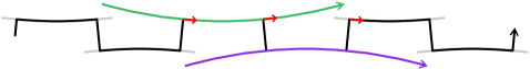
Figure 8. Case I, $g$ and $h$ hyperbolic. $T_{h}$ is green, $T_{g}$ is purple, $T_{gh}$ is black. The red edges are of the form $e$, $he$, and $ghe$.

Note that $gh$ has a fundamental domain given by the concatenation $\alpha\cdot\rho\cdot\beta\cdot\rho^{\prime}$, by Remark 6.3. More generally, $(gh)^{n}$ has a fundamental domain made of $n$ copies each of $\alpha$, $\rho$, $\beta$, and $\overline{\rho}$. Lemma 6.5 yields

$$n(c_{\gamma}(\alpha)+c_{\gamma}(\rho)+c_{\gamma}(\beta)+c_{\gamma}(\overline{\rho}))\ \leqslant\ c_{\gamma}((gh)^{n})\$$

$$\leqslant\ n(c_{\gamma}(\alpha)+c_{\gamma}(\rho)+c_{\gamma}(\beta)+c_{\gamma}(\overline{\rho}))+4n$$ (19)

and

$$n(c_{\overline{\gamma}}(\alpha)+c_{\overline{\gamma}}(\rho)+c_{\overline{\gamma}}(\beta)+c_{\overline{\gamma}}(\overline{\rho}))\ \leqslant\ c_{\overline{\gamma}}((gh)^{n})\$$

$$\leqslant\ n(c_{\overline{\gamma}}(\alpha)+c_{\overline{\gamma}}(\rho)+c_{\overline{\gamma}}(\beta)+c_{\overline{\gamma}}(\overline{\rho}))+4n.$$ (20)

Subtracting (6) from (6) yields

$$n(f_{\gamma}(\alpha)+f_{\gamma}(\beta))-4n\ \leqslant\ f_{\gamma}((gh)^{n})\ \leqslant\ n(f_{\gamma}(\alpha)+f_{\gamma}(\beta))+4n.$$ (21)

Since $h^{n}$ and $g^{n}$ have fundamental domains made of $n$ copies of $\alpha$ and $\beta$ respectively, Lemma 6.5 also yields, in a similar way,

$$nf_{\gamma}(\alpha)-n\ \leqslant\ f_{\gamma}(h^{n})\ \leqslant\ nf_{\gamma}(\alpha)+n$$ (22)

and

$$nf_{\gamma}(\beta)-n\ \leqslant\ f_{\gamma}(g^{n})\ \leqslant\ nf_{\gamma}(\beta)+n.$$ (23)

Subtracting (22) and (23) from (21) yields

$$-6n\ \leqslant\ f_{\gamma}((gh)^{n})-f_{\gamma}(g^{n})-f_{\gamma}(h^{n})\ \leqslant\ 6n.$$

Dividing by $n$ and taking a limit, we obtain $\left\lvert{h_{\gamma}(gh)-h_{\gamma}(g)-h_{\gamma}(h)}\right\rvert\ \leqslant\ 6$, as desired.

Remark. In the argument just given, the fundamental domains for $h$, $g$, and $gh$ respectively were decomposed into one, one, and four segments; hence $T_{h}/\langle h\rangle$, $T_{g}/\langle g\rangle$, and $T_{gh}/\langle gh\rangle$ contained a total of six junctures. These junctures were the only source of defect, since the individual segments always contributed zero to $\left\lvert{f_{\gamma}(gh)-f_{\gamma}(g)-f_{\gamma}(h)}\right\rvert$. Every case below follows the same pattern: the defect will be bounded above by the total number of junctures appearing in the quotient circuits. In what follows, we will describe the structure of $T_{h}/\langle h\rangle$, $T_{g}/\langle g\rangle$, and $T_{gh}/\langle gh\rangle$ in each case and leave some of the details of the estimates to the reader.

Returning to Case I, suppose $g$ and $h$ are both elliptic. Then $g^{n}$ and $h^{n}$ are also elliptic, and $(gh)^{n}$ has a fundamental domain made of $n$ copies of $\rho$ and $n$ copies of $\overline{\rho}$. See Figure 9. Using Lemma 6.5 one obtains

$$\left\lvert{f_{\gamma}((gh)^{n})-f_{\gamma}(g^{n})-f_{\gamma}(h^{n})}\right\rvert\ =\ \left\lvert{f_{\gamma}((gh)^{n})}\right\rvert\ \leqslant\ 2n,$$

for a defect of at most $2$.

2pt $\rho$ [tr] at 111 24 $T_{h}$ [c] at 92 42 $T_{g}$ [c] at 129 7 $T_{gh}$ [l] at 293 26

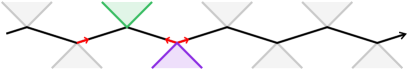
Figure 9. Case I, $g$ and $h$ elliptic. $T_{h}$ is green, $T_{g}$ is purple, $T_{gh}$ is black. The red edges are of the form $e$, $he$, and $ghe$.

If one of $g$ and $h$ is elliptic, say $g$, then $h^{n}$ has a fundamental domain given by $n$ copies of $\alpha$, and $(gh)^{n}$ has a fundamental domain given by $n$ copies each of $\alpha$, $\rho$, and $\overline{\rho}$. The estimate given by Lemma 6.5 becomes

$$\left\lvert{f_{\gamma}((gh)^{n})-f_{\gamma}(g^{n})-f_{\gamma}(h^{n})}\right\rvert\ =\ \left\lvert{f_{\gamma}((gh)^{n})-f_{\gamma}(h^{n})}\right\rvert\ \leqslant\ 4n,$$

for a defect of at most $4$.

Case II: $g$ and $h$ are hyperbolic, with positive overlap. That is, $T_{g}$ and $T_{h}$ intersect in a segment, on which $T_{g}$ and $T_{h}$ induce the same orientation. Let $e$ be an edge in $T_{g}\cap T_{h}$, oriented coherently with $T_{g}$ and $T_{h}$. Let $v$ be the terminal vertex of $e$. Since $e\in T_{h}$, the edges $h^{-1}e$ and $e$ are coherently oriented and $\alpha=[h^{-1}v,v]$ is a fundamental domain for $h$. Similarly, $e$ and $ge$ are coherently oriented and $\beta=[v,gv]$ is a fundamental domain for $g$.

Let all the edges of $\alpha$ and $\beta$ be given orientations from $T_{h}$ and $T_{g}$ respectively. Since $g$ and $h$ both move $e$ in the same direction (that is, into the same component of $T-\{e\}$), $e$ separates $h^{-1}e$ from $ge$. It follows that the edges of $\alpha$ and of $\beta$ are all coherently oriented in $T$. Hence $\alpha$ and $\beta$ do not overlap, and $\alpha\cdot\beta=[h^{-1}v,gv]$ is a fundamental domain for $gh$.

With a total of four junctures (one for $h$, one for $g$, two for $gh$), the estimate given by Lemma 6.5 becomes

$$\left\lvert{f_{\gamma}((gh)^{n})-f_{\gamma}(g^{n})-f_{\gamma}(h^{n})}\right\rvert\ \leqslant\ 4n,$$

for a defect of at most $4$.

Case III: $g$ and $h$ are hyperbolic, with negative overlap. That is, $T_{g}$ and $T_{h}$ intersect in a segment, on which $T_{g}$ and $T_{h}$ induce opposite orientations. Let $\Delta$ be the length (possibly infinite) of $T_{g}\cap T_{h}$. There are several sub-cases, according to the relative sizes of $\left\lvert{g}\right\rvert$, $\left\lvert{h}\right\rvert$, and $\Delta$.

Sub-case III-A: $\Delta\leqslant\left\lvert{g}\right\rvert,\left\lvert{h}\right\rvert$, not all three numbers equal. Let $\rho$ be the segment $T_{h}\cap T_{g}$, oriented coherently with $T_{h}$. There is a fundamental domain for $h$ of the form $\alpha\cdot\rho$, and similarly, a fundamental domain for $g$ of the form $\overline{\rho}\cdot\beta$; see Figure 10. Then $\alpha\cdot\beta$ is a fundamental domain for $gh$. (By assumption, at least one of $\alpha$, $\beta$ is a non-trivial segment, and $gh$ is hyperbolic.)

2pt $\alpha$ [tl] at 102 21 $\beta$ [tr] at 137 19 $\rho$ [r] at 112 50 $T_{h}$ [l] at 149 97 $T_{g}$ [l] at 183 2 $T_{gh}$ [l] at 318 20

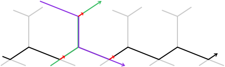
Figure 10. Case III-A. $T_{h}$ is green, $T_{g}$ is purple, $T_{gh}$ is black. The red edges are of the form $e$, $he$, and $ghe$.

The quotient circuits have at most six junctures: two for $g$, two for $h$, and two for $gh$. Lemma 6.5 leads to an estimate

$$\left\lvert{f_{\gamma}((gh)^{n})-f_{\gamma}(g^{n})-f_{\gamma}(h^{n})}\right\rvert\ \leqslant\ 6n,$$

for a defect of at most $6$.

Sub-case III-B: $\left\lvert{g}\right\rvert=\left\lvert{h}\right\rvert\leqslant\Delta$. In this case, we show that $gh$ is elliptic. Let $\alpha\subset T_{h}\cap T_{g}$ be a fundamental domain for $h$. Then $\overline{\alpha}$ is a fundamental domain for $g$, and $gh$ fixes the initial endpoint of $\alpha$. With two junctures in total, we obtain the estimate

$$\left\lvert{f_{\gamma}((gh)^{n})-f_{\gamma}(g^{n})-f_{\gamma}(h^{n})}\right\rvert\ =\ \left\lvert{-f_{\gamma}(g^{n})-f_{\gamma}(h^{n})}\right\rvert\ \leqslant\ 2n,$$

for a defect of at most $2$.

Sub-case III-C: $\left\lvert{h}\right\rvert<\left\lvert{g}\right\rvert,\Delta$. There is a simplicial fundamental domain $\alpha$ for $h$ such that if $e$ is the initial edge of $\alpha$, then $\alpha\cdot he$ is contained in $T_{h}\cap T_{g}$. Then, there is a fundamental domain for $g$ of the form $\overline{\alpha}\cdot\beta$; see Figure 11. By considering the location of $ghe$, one finds that $\beta$ is a fundamental domain for $gh$. The three circuits have a total of four junctures, and we obtain

$$\left\lvert{f_{\gamma}((gh)^{n})-f_{\gamma}(g^{n})-f_{\gamma}(h^{n})}\right\rvert\ \leqslant\ 4n,$$

for a defect of at most $4$.

2pt $\alpha$ [b] at 58 34 $\beta$ [tl] at 26 23 $\alpha$ [bl] at 185 39 $\beta$ [t] at 227 25 $e$ [tl] at 48 14 $he$ [tl] at 89 14 $ghe$ [b] at 7 30 $e$ [t] at 165 37 $he$ [b] at 248 48 $ghe$ [b] at 221 46.5 $T_{h}$ [tl] at 128 57 $T_{g}$ [r] at 2 3 $T_{h}$ [tl] at 290 57 $T_{g}$ [r] at 164 3

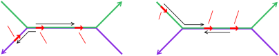
Figure 11. Cases III-C (left) and III-D (right). $T_{h}$ is green, $T_{g}$ is purple.

Sub-case III-D: $\left\lvert{g}\right\rvert<\left\lvert{h}\right\rvert,\Delta$. Fundamental domains $\beta$, $\alpha$, and $\alpha\cdot\overline{\beta}$ for $g$, $gh$, and $h$ respectively can be constructed in a similar fashion as in Case III-C; see Figure 11. Alternatively, this case reduces to Case III-C, replacing $g$ and $h$ by $h^{-1}$ and $g^{-1}$ respectively.

Case IV: $g$ is elliptic, $h$ is hyperbolic, $T_{g}\cap T_{h}\not=\emptyset$. If $T_{g}\cap T_{h}$ contains an edge $e$, let $\alpha\subset T_{h}$ be the fundamental domain starting with $h^{-1}e$. Then $\alpha$ is also a fundamental domain for $gh$. This leads to an estimate

$$\left\lvert{f_{\gamma}((gh)^{n})-f_{\gamma}(g^{n})-f_{\gamma}(h^{n})}\right\rvert\ =\ \left\lvert{f_{\gamma}((gh)^{n})-f_{\gamma}(h^{n})}\right\rvert\ \leqslant\ 2n,$$

and a defect of at most $2$.

If $T_{g}\cap T_{h}$ is a single vertex $v$, let $e\in T_{h}$ be the coherently oriented edge with initial vertex $v$, and let $\alpha$ be the fundamental domain $[h^{-1}v,v]$. If $ge\not\in\alpha$ then $\alpha$ is a fundamental domain for $gh$ also, and we obtain a defect of at most $2$ as above.

So now assume that $ge\in\alpha$, i.e. that $ge$ separates $h^{-1}v$ from $v$. Note that $h^{-1}e$ and $ge$ are not coherently oriented, so the characteristic subtree $T_{gh}$ will not contain these edges.

We have that $gh(\alpha)\cap\alpha$ contains the edge $ge$. Consider the length of $gh(\alpha)\cap\alpha$. If this length is $\left\lvert{\alpha}\right\rvert/2$ or greater, then $gh$ fixes the midpoint of $\alpha$. Then

$$\left\lvert{f_{\gamma}((gh)^{n})-f_{\gamma}(g^{n})-f_{\gamma}(h^{n})}\right\rvert\ =\ \left\lvert{-f_{\gamma}(h^{n})}\right\rvert\ \leqslant\ n,$$

giving a defect of at most $1$.

Otherwise, there is a subsegment $\beta\subset\alpha$, centered on the midpoint of $\alpha$, of maximal size so that $\beta$ does not overlap $gh\beta$. We can write $\alpha$ as a concatenation $\alpha_{1}\cdot\beta\cdot\alpha_{2}$, where $\alpha_{2}=gh\overline{\alpha}_{1}$. See Figure 12.

2pt $\alpha_{1}$ [b] at 46 13 $\alpha_{2}$ [b] at 117 31 $gh\alpha_{2}$ [b] at 46 49 $\beta$ [tl] at 83 19 $gh\beta$ [tr] at 81 36 $T_{h}$ [l] at 187 26 $T_{g}$ [c] at 147 14 $T_{gh}$ [r] at 82 73

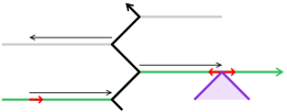
Figure 12. Case IV. The element $gh$ takes $\alpha_{1}$ to $\overline{\alpha}_{2}$. Left to right, the red edges are $h^{-1}e$, $ge$, and $e$.

Now $\beta$ is a fundamental domain for $gh$, and we have a total of four junctures (three in $T_{h}/\langle h\rangle$ and one in $T_{gh}/\langle gh\rangle$). Thus we have

$$\left\lvert{f_{\gamma}((gh)^{n})-f_{\gamma}(g^{n})-f_{\gamma}(h^{n})}\right\rvert\ =\ \left\lvert{f_{\gamma}((gh)^{n})-f_{\gamma}(h^{n})}\right\rvert\ \leqslant\ 4n,$$

and a defect of at most $4$.

Case V: $h$ is elliptic, $g$ is hyperbolic, $T_{g}\cap T_{h}\not=\emptyset$. This case is covered by Case IV, replacing $g$ and $h$ by $h^{-1}$ and $g^{-1}$ respectively.

Case VI: the remaining cases. If $g$ and $h$ are hyperbolic and $T_{g}$ and $T_{h}$ intersect in one point, then the configuration closely resembles the first one discussed in Case I, except that the copies of $\rho$ have been shrunk to have length zero. That is, there are fundamental domains $\alpha$ and $\beta$ for $h$ and $g$ respectively, such that $\alpha\cdot\beta$ is a fundamental domain for $gh$. With four junctures, we obtain

$$\left\lvert{f_{\gamma}((gh)^{n})-f_{\gamma}(g^{n})-f_{\gamma}(h^{n})}\right\rvert\ \leqslant\ 4n,$$

for a defect of at most $4$.

Lastly, if $g$ and $h$ have a common fixed point, then

$$\left\lvert{f_{\gamma}((gh)^{n})-f_{\gamma}(g^{n})-f_{\gamma}(h^{n})}\right\rvert\ =\ 0$$

for all $n$. ∎

Remark 6.7.

The functions $f_{\gamma}$ and $h_{\gamma}$ can be defined in the more general setting of a group acting on an ${\mathbb{R}}$–tree. The proof of Theorem 6.6 goes through in this setting, with only superficial modifications (essentially, removing any mention of edges, and using small segments instead).

Well-aligned elements

We now consider elements $g\in G$ for which we can find a segment $\gamma\subset T$ such that $h_{\gamma}(g)=1$.

Definition 6.8.

Given a $G$–tree $T$, a hyperbolic element $g\in G$ is well-aligned if there does not exist an element $h\in G$ such that $ghgh^{-1}$ fixes an edge of $T_{g}$. This property is the $G$–tree analogue of the double coset condition from [9, Theorem D].

Theorem 6.9.

Suppose $G$ acts on a simplicial tree $T$. If $g\in G$ is well-aligned then $\operatorname{scl}(g)\geqslant 1/12$.

Proof.

Let $\gamma=[x,gx]\subset T_{g}$ be a fundamental domain for $g$ where $x$ is not a vertex of $T$. We know that $c_{\gamma}(g^{n})=n$ for all $n$. If $c_{\overline{\gamma}}(g^{n})>0$ for some $n$, then there is a copy of $\overline{\gamma}$ in $T_{g}$. That is, there is an element $h$ such that $h\gamma$ lies in $T_{g}$ with the opposite orientation. So $h(T_{g})=T_{hgh^{-1}}$ has negative overlap with $T_{g}$ along a segment containing $h\gamma$. The element $ghgh^{-1}$ fixes one of the endpoints of $h\gamma$, since $g$ and $hgh^{-1}$ shift it in opposite directions inside $T_{g}\cap T_{hgh^{-1}}$. This endpoint is in the interior of an edge $e\subset T_{g}$, and so $ghgh^{-1}$ fixes $e$. Hence, if $g$ is well-aligned, we must have $h_{\gamma}(g)=1$. By Theorem 6.6, $h_{\gamma}$ is a homogeneous quasimorphism with defect at most $6$, and so Proposition 6.2 implies that $\operatorname{scl}(g)\geqslant 1/12$. ∎

This bound is in fact optimal. Both in HNN extensions and in amalgamated free products, there are examples of elements $g$ with $\operatorname{scl}(g)=1/12$ that are well-aligned with respect to the action on the associated Bass–Serre tree, as we now explain. This answers Question 8.4 from [9].

Theorem 6.10.

Let $g=tat^{-1}a\in BS(2,3)$ and let $T$ be the Bass–Serre tree associated to the splitting of $BS(2,3)$ as an HNN extension $\langle a\rangle*_{\langle ta^{2}t^{-1}=a^{3}\rangle}$. Then $g$ is well-aligned and $\operatorname{scl}(g)=1/12$. In particular, the bound in Theorem 6.9 is optimal.

Proof.

Denote the vertex of $T$ stabilized by $\langle a\rangle$ by $v_{0}$ and let $v_{1}=tv_{0}$. The vertices along the axis of $g$ are: $\{g^{n}v_{0},g^{n}v_{1}\}_{n\in{\mathbb{Z}}}$.

If $ghgh^{-1}$ fixes an edge $e\subset T_{g}$, then we also see that $hgh^{-1}g$ fixes $g^{-1}e\subset T_{g}$. Replacing $h$ by $hg^{k}$ for some $k$ (which does not affect $hgh^{-1}$), we can arrange that $h$ fixes a vertex of $T_{g}$. By further replacing $h$ by a conjugate $g^{k}hg^{-k}$, we can arrange that the vertex fixed by $h$ is either $v_{0}$ or $v_{1}$; the elements $ghgh^{-1}$ and $hgh^{-1}g$ still fix edges of $T_{g}$.

First assume that $h$ fixes $v_{0}$, and so $h=a^{r}$ for some $r\in{\mathbb{Z}}$. In this case

$$ghgh^{-1}=tat^{-1}a^{1+r}tat^{-1}a^{1-r}.$$

If $ghgh^{-1}$ is elliptic (which it necessarily is if it fixes an edge), then this expression cannot be cyclically reduced (Remark 2.6). Hence we find that $r\equiv\pm 1\mod 3$. If $r\equiv 1\mod 3$, then $hgh^{-1}g=a^{5}$; if $r\equiv-1\mod 3$ then $ghgh^{-1}=a^{5}$. In either case, the element does not fix an edge in $T$, giving a contradiction.

Similarly, if $h$ fixes $v_{1}$, then we have $h=ta^{r}t^{-1}$ for some $r\in{\mathbb{Z}}$, and so

$$hgh^{-1}g=ta^{1+r}t^{-1}ata^{1-r}t^{-1}a.$$

Again, this expression cannot be cyclically reduced if $hgh^{-1}g$ is elliptic, and so $r\equiv 1\mod 2$. Again, we find that $hgh^{-1}g=a^{5}$, giving a contradiction for the same reason as above. Therefore $g$ is well-aligned as claimed.

Finally, $\operatorname{scl}(tat^{-1}a)=1/12$ by Proposition 5.5. ∎

The bound in Theorem 6.9 is still optimal if one restricts to amalgamated free products. In the free product ${\mathbb{Z}}/2{\mathbb{Z}}*{\mathbb{Z}}/3{\mathbb{Z}}\cong\operatorname{PSL}(2,{\mathbb{Z}})$, no nontrivial element fixes an edge of the associated Bass–Serre tree, so every hyperbolic element that is not conjugate to its inverse is well-aligned. The group $\operatorname{PSL}(2,{\mathbb{Z}})$ has a finite index free subgroup, and therefore stable commutator length can be computed in this group by using a relationship between stable commutator length in a group and a finite index subgroup from [6] together with Calegari’s algorithm for computing stable commutator length in free groups [7]. This is described explicitly in [16]. The element $\bigl{(}\begin{smallmatrix}1&0\\ 1&1\end{smallmatrix}\bigr{)}$ is an example of an element that has stable commutator length $1/12$.

Acylindrical trees

We conclude this section by adding a moderate restriction, acylindricity, to the tree action. We can then say something about hyperbolic elements that are not necessarily well-aligned.

Acylindricity has been used previously in the context of counting quasimorphisms on Gromov-hyperbolic spaces, cf. [9]. For a tree, the definition is particularly simple to state. A group acts $K$–acylindrically on a tree if the stabilizer of any segment of length $K$ is trivial.

Theorem 6.11.

Suppose $G$ acts $K$–acylindrically on a tree $T$ and let $N$ be the smallest integer greater than or equal to $\frac{K}{2}+1$.

1. If $g\in G$ is hyperbolic then either $\operatorname{scl}(g)=0$ or $\operatorname{scl}(g)\geqslant 1/12N$.

2. If $g\in G$ is hyperbolic and $\left\lvert{g}\right\rvert\geqslant K$ then either $\operatorname{scl}(g)=0$ or $\operatorname{scl}(g)\geqslant 1/24$.

In both cases, $\operatorname{scl}(g)=0$ if and only if $g$ is conjugate to $g^{-1}$.

Proof.

First note that if $\left\lvert{g}\right\rvert=1$ then a fundamental domain for $g$ maps to a single loop in the quotient graph of $T$, which implies that $g$ has infinite order in the abelianization of $G$, and $\operatorname{scl}(g)=\infty$. (In fact, the same conclusion holds whenever $\left\lvert{g}\right\rvert$ is odd.) Thus we may assume that $\left\lvert{g}\right\rvert\geqslant 2$.

Observe that if for some $h\in G$, we have $\left\lvert{T_{g}\cap T_{hgh^{-1}}}\right\rvert\geqslant K+\left\lvert{g}\right\rvert$ where $g$ and $hgh^{-1}$ shift in opposite directions, then $ghgh^{-1}$ fixes a segment of length $K$ and hence $g=hg^{-1}h^{-1}$. In particular, $\operatorname{scl}(g)=0$.

For (i) note that $\left\lvert{g^{N}}\right\rvert=N\left\lvert{g}\right\rvert\geqslant\frac{K}{2}\left\lvert{g}\right\rvert+\left\lvert{g}\right\rvert\geqslant K+\left\lvert{g}\right\rvert$. Taking $\gamma$ to be a fundamental domain for $g^{N}$, if $h_{\gamma}(g^{N})<1$ then there is an $h$ as above and $g=hg^{-1}h^{-1}$, $\operatorname{scl}(g)=0$. Otherwise, $h_{\gamma}(g^{N})=1$ and $\operatorname{scl}(g)=\frac{1}{N}\operatorname{scl}(g^{N})\geqslant 1/12N$ by Theorem 6.6 and Proposition 6.2.

For (ii) let $N=2$ and apply the same reasoning: $\left\lvert{g^{2}}\right\rvert=2\left\lvert{g}\right\rvert\geqslant K+\left\lvert{g}\right\rvert$, and either $\operatorname{scl}(g)=0$ or $\operatorname{scl}(g)=\frac{1}{2}\operatorname{scl}(g^{2})\geqslant 1/24$. ∎

7. The gap theorem

In this section we consider $G$–trees of a particular form, for which we can improve upon the “well-aligned” condition in Theorem 6.9 without any trade-off in the lower bound of $1/12$.

Let $G$ be an HNN extension $A\,\ast_{C}$, with stable letter $t$, such that the edge groups $C$ and $C^{t}$ are central in $A$. Let $T$ be the Bass–Serre tree associated to this HNN extension. Such a tree has special properties, given below in Lemma 7.1 and Proposition 7.2.

This class of HNN extensions obviously includes the Baumslag–Solitar groups. It is still true (cf. Remark 2.4) that an element cannot have finite stable commutator length if its $t$–exponent is non-zero.

We use the following notation for a $G$–tree $T$: if $X\subset T$ is any subset, then $G_{X}$ denotes the stabilizer of $X$, which is the subgroup of $G$ consisting of those elements that fix $X$ pointwise.

Lemma 7.1.

Suppose $S\subset T$ is a subtree and $h\in G$ fixes a vertex $v\in S$. Then $G_{S}=G_{hS}$.

Proof.

Let $e$ be an edge in $S$ with endpoint $v$. Then $G_{S}\subset G_{e}$. Since $G_{e}$ is central in $G_{v}$, $h$ commutes with $G_{S}$, and therefore $G_{hS}=hG_{S}h^{-1}=G_{S}$. ∎

Consider the $t$–exponent homomorphism $\phi\colon\thinspace G\to{\mathbb{Z}}$ (sending $t$ to $1$ and $A$ to $0$). There is an action of ${\mathbb{Z}}$ on ${\mathbb{R}}$ by integer translations. Letting $G$ act on ${\mathbb{R}}$ via $\phi$, there is also a $G$–equivariant map $F\colon\thinspace T\to{\mathbb{R}}$. This map is just the natural map from $T$ to the universal cover of the quotient graph $T/G$. The action of an element $g$ on $T$ projects by $F$ to a translation by $\phi(g)$ on ${\mathbb{R}}$. We think of $F$ as a height function on $T$. Then, the elements of $t$–exponent zero act on $T$ by height-preserving automorphisms.

Proposition 7.2.

If $S\subset T$ is a subtree and $\sigma\subset S$ is a finite subtree such that $F(\sigma)=F(S)$ then $G_{\sigma}=G_{S}$.

Proof.

Case I: $\sigma$ is a segment mapped by $F$ injectively to ${\mathbb{R}}$.

First suppose that $S$ is a finite subtree. Let $\{S_{i}\}$ be the subtrees obtained as the closures of the components of $S-\sigma$. Then $G_{S}=G_{\sigma}\cap\bigcap_{i}G_{S_{i}}$. Fixing $i$, we will prove by induction on the number of edges of $S_{i}$ that $G_{\sigma}\subset G_{S_{i}}$. It then follows that $G_{\sigma}=G_{S}$.

The base case is that $S_{i}$ is a single edge $e$ with one vertex $v$ on $\sigma$. Since $F(S_{i})\subset F(\sigma)$, there is an edge $e^{\prime}$ on $\sigma$ with endpoint $v$ and an element $h\in G_{v}$ taking $e$ to $e^{\prime}$. Indeed, edges incident to $v$ are in the same $G_{v}$–orbit if and only if they have the same image under $F$. By Lemma 7.1 we have that $G_{S_{i}}=G_{e^{\prime}}\supset G_{\sigma}$.

For larger $S_{i}$, let $e\in S_{i}$ be the edge with endpoint $v\in\sigma$. Again there is an edge $e^{\prime}$ on $\sigma$ with endpoint $v$ and an element $h\in G_{v}$ taking $e$ to $e^{\prime}$. Again, $G_{S_{i}}=G_{hS_{i}}$ by Lemma 7.1. But now $hS_{i}=e^{\prime}\cup S_{i}^{\prime}$ where $S_{i}^{\prime}$ has fewer edges than $S_{i}$. By induction, $G_{\sigma}\subset G_{S_{i}^{\prime}}$. Since $G_{\sigma}\subset G_{e^{\prime}}$, we now have $G_{\sigma}\subset(G_{e^{\prime}}\cap G_{S_{i}^{\prime}})=G_{S_{i}}$.

Now consider an arbitrary subtree $S$. We need to show that $G_{\sigma}$ fixes $S$ pointwise. But every point $x$ in $S$ is in a finite subtree $S^{\prime}$ containing $\sigma$, and $G_{\sigma}$ fixes $S^{\prime}$ pointwise; hence $G_{\sigma}$ fixes $x$.

Case II: $\sigma$ is an arbitrary finite subtree of $S$. Fixing the image $F(\sigma)$, we proceed by induction on the number of edges of $\sigma$. The base case is when this number is smallest, namely the length of $F(\sigma)$. Then Case I applies. If there are more edges than this, there must be a vertex $v\in\sigma$ and a pair of edges $e_{0},e_{1}\in\sigma$ incident to $v$, with $F(e_{0})=F(e_{1})$.

Decompose $S$ into two subtrees $S=S_{0}\cup S_{1}$ with $S_{0}\cap S_{1}=\{v\}$ and $e_{0}\in S_{0}$, $e_{1}\in S_{1}$. Let $\sigma_{i}=S_{i}\cap\sigma$. There is an element $h\in G_{v}$ such that $he_{0}=e_{1}$. Let $\sigma^{\prime}=h\sigma_{0}\cup\sigma_{1}$ and $S^{\prime}=hS_{0}\cup S_{1}$. Note that $\sigma^{\prime}$ has fewer edges than $\sigma$. Also, $F(\sigma)=F(\sigma^{\prime})$ and $F(S)=F(S^{\prime})$, and $G_{\sigma}=G_{\sigma_{0}}\cap G_{\sigma_{1}}=G_{h\sigma_{0}}\cap G_{\sigma_{1}}=G_{\sigma^{\prime}}$ by Lemma 7.1. Similarly, $G_{S}=G_{S_{0}}\cap G_{S_{1}}=G_{hS_{0}}\cap G_{S_{1}}=G_{S^{\prime}}$. By the induction hypothesis, $G_{\sigma^{\prime}}=G_{S^{\prime}}$, and therefore $G_{\sigma}=G_{S}$. ∎

Now consider a hyperbolic element $g$ with $t$–exponent zero. The axis $T_{g}$ has the property that $F(T_{g})$ is a finite interval. To see this, let $\gamma$ be a fundamental domain, and note that $T_{g}=\bigcup_{n}g^{n}\gamma$. The $t$–exponent condition implies that $F(g^{n}\gamma)=F(\gamma)$ for all $n$, and hence $F(T_{g})=F(\gamma)$.

Definitions 7.3.

We call a vertex $v$ on $T_{g}$ extremal if $F(v)$ is an endpoint of $F(T_{g})$. A segment $\sigma\subset T_{g}$ is stable if $F(\sigma)=F(T_{g})$ and $\sigma$ contains no extremal vertex in its interior (equivalently, no proper subsegment $\sigma^{\prime}$ satisfies $F(\sigma^{\prime})=F(T_{g})$). See Figure 13. Note that if $\sigma$ and $\tau$ are stable segments, then they do not overlap, unless they are equal.

2pt $T_{g}$ [c] at 75 19 $F$ [b] at 312 30

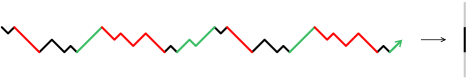
Figure 13. Stable segments along $T_{g}$, in green and red.

The natural orientation of $T_{g}$ defines a linear ordering $<_{g}$ on the stable segments of $T_{g}$. The “larger” end is the attracting end of $T_{g}$; that is, $\sigma<_{g}g\sigma$ always holds. We say that $\sigma\leqslant_{g}\tau$ if $\sigma<_{g}\tau$ or $\sigma=\tau$.

Remark 7.4.

If $\gamma$ is a fundamental domain for $g$ whose endpoints are extremal, then every stable segment either does not overlap with $\gamma$ or is contained in $\gamma$. Moreover, $\gamma$ contains a copy of every stable segment. (Being a fundamental domain, it overlaps with a copy of every non-trivial segment in $T_{g}$.) If $\gamma$ is a fundamental domain that starts with a stable segment then its endpoints are extremal, as the endpoints of a stable segment are extremal.

Proposition 7.2 immediately implies:

Corollary 7.5.

If $\sigma\subset T_{g}$ is stable then $G_{\sigma}=G_{T_{g}}$.

The main technical result of this section is:

Theorem 7.6.

Let $G=A\,\ast_{C}$ with stable letter $t$, and $C,C^{t}$ central in $A$. Let $g\in G$ be a hyperbolic element with $t$–exponent zero. Then either:

1. there is a fundamental domain $\gamma$ for $g$ such that $h_{\gamma}(g)=1$, or

2. there is an element $h$ such that $h(T_{g})=\overline{T}_{g}$.

Conclusion (i) implies by Proposition 6.2 and Theorem 6.6 that $\operatorname{scl}(g)\geqslant 1/12$.

Proof.

Let $\alpha\subset T_{g}$ be a stable segment and let $\gamma$ be the fundamental domain for $g$ that starts with $\alpha$. Note that $\gamma$ has extremal endpoints. If $h_{\gamma}(g)<1$ then there is an element $h$ such that $h\gamma$ lies in $T_{g}$ with the opposite orientation and overlaps with $\alpha$. Note that $h$ fixes a point in $\gamma$. In particular $h$ is elliptic, and hence acts as a height-preserving automorphism of $T$. Now $h\gamma$ is a fundamental domain for $g^{-1}$ with extremal endpoints, and so $h\gamma$ contains $\alpha$ (which is stable for $T_{g^{-1}}$ as well as for $T_{g}$).

The segment $\beta=h^{-1}\alpha$ is a stable segment for $T_{g}$ contained in $\gamma$. Clearly $\alpha\leqslant_{g}\beta$, and as the endpoints of $\alpha$ have different heights, $\alpha\neq\beta$; therefore $\alpha<_{g}\beta$. Note that $h\alpha=\beta$, since $h$ acts as a reflection on the segment $\gamma\cap h\gamma$. Hence the element $h^{2}$ fixes the stable segment $\alpha$. Therefore, by Proposition 7.2, $h^{2}$ fixes $T_{g}\cup h(T_{g})$. That is, $h$ acts as an involution on this entire subtree of $T$.

Claim.

If there is a stable segment $\rho\subset T_{g}\cap h(T_{g})$ such that either $\rho<_{g}\alpha$ or $\beta<_{g}\rho$, then conclusion (ii) holds.

Proof of Claim.

Since $h$ acts as a reflection on the segment $T_{g}\cap h(T_{g})$, if $\rho\subset T_{g}\cap h(T_{g})$ and $\rho<_{g}\alpha$, then $h\rho\subset T_{g}\cap h(T_{g})$ and $\beta<_{g}h\rho$. Thus we only need to verify the claim in the $\beta<_{g}\rho$ case.

Let $\sigma$ be the $<_{g}$–smallest stable segment in $h\gamma$. Observe that $\sigma\subset T_{g}\cap h(T_{g})$. The translate $g\sigma$ is the $<_{g}$–smallest stable segment in $gh\gamma$, which has a common endpoint with $\beta$. Hence $g\sigma\leqslant_{g}\tau$ for any $\tau$ satisfying $\beta<_{g}\tau$. In particular, $g\sigma\leqslant_{g}\rho$. Since $\beta,\rho\subset T_{g}\cap h(T_{g})$ and $\beta<_{g}g\sigma\leqslant_{g}\rho$, it follows that $g\sigma\subset T_{g}\cap h(T_{g})$.

Note that $h(T_{g})=T_{hgh^{-1}}$, and $hgh^{-1}$ takes $g\sigma$ to $\sigma$. Thus $ghgh^{-1}$ fixes $g\sigma$. Since this is a stable segment, $ghgh^{-1}$ must fix all of $T_{g}$ by Corollary 7.5. This implies that $hgh^{-1}$ acts on $T_{g}$ as a translation, of the same amplitude but opposite direction as $g$. Hence $T_{hgh^{-1}}=\overline{T}_{g}$. ∎

Returning to the proof of Theorem 7.6, assume that the Claim does not apply. Then $\alpha$ and $\beta$ are the $<_{g}$–smallest and $<_{g}$–largest stable segments in $T_{g}\cap h(T_{g})$ respectively. It follows that $\beta$ is also the $<_{g}$–largest stable segment in $\gamma$; otherwise, if $\beta<_{g}\rho$ and $\rho\subset\gamma$, then $h\rho<_{g}\alpha$ and $h\rho\subset T_{g}\cap h(T_{g})$, contradicting that $\alpha$ is smallest.

Note that $h$ takes stable segments to stable segments, and does not take any stable segment to itself (since the endpoints have different heights). Hence the stable segments of $\gamma$ may be enumerated in order as $\alpha=\alpha_{1},\ldots,\alpha_{n},\beta_{n},\ldots,\beta_{1}=\beta$ where $h$ interchanges $\alpha_{i}$ and $\beta_{i}$.

Now let $\gamma^{\prime}$ be the fundamental domain for $g$ starting with $\beta_{n}$. Assuming that conclusion (i) does not hold, we have $h_{\gamma^{\prime}}(g)<1$, and so there is an elliptic element $k$ such that $k\gamma^{\prime}$ lies in $T_{g}$ with the opposite orientation and contains $\beta_{n}$.

The configuration of $T_{g}$, $k(T_{g})$, $\beta_{n}$, and $k\beta_{n}$ is exactly analogous to that of $T_{g}$, $h(T_{g})$, $\alpha$, and $\beta$. In particular, the Claim is applicable to this situation. If the Claim does not apply, then we conclude as above that $\beta_{n}$ and $k\beta_{n}$ are the $<_{g}$–smallest and $<_{g}$–largest stable segments in $T_{g}\cap k(T_{g})$ and that $k\beta_{n}$ is the $<_{g}$–largest stable segment in $\gamma^{\prime}$.

The stable segments in $\gamma^{\prime}$ are, in order: $\beta_{n},\ldots,\beta_{1},g\alpha_{1},\ldots,g\alpha_{n}$, and the element $k$ interchanges $\beta_{i}$ and $g\alpha_{i}$. Thus

$$kh\alpha=kh\alpha_{1}=k\beta_{1}=g\alpha_{1}=g\alpha.$$

Since $kh$ and $g$ agree on the stable segment $\alpha$, they agree on all of $T_{g}\cup h(T_{g})\cup k(T_{g})$, by Proposition 7.2. Similarly, $h$ and $k$ both act as involutions on $T_{g}\cup h(T_{g})\cup k(T_{g})$. Now

$$hg^{-1}\beta=h(kh)^{-1}\beta=hhk\beta=k\beta=g\alpha,$$

which implies that $g\alpha\subset T_{g}\cap h(T_{g})$. However, $\beta<_{g}g\alpha$ and $\beta$ is the $<_{g}$–largest stable segment in $T_{g}\cap h(T_{g})$. This contradiction establishes the theorem. ∎

The next proposition concerns conclusion (ii) in Theorem 7.6. It is a variant of the observation that if an element is conjugate to its inverse, then it has $\operatorname{scl}$ zero.

Proposition 7.7.

Suppose $G$ acts on a tree $T$ and $\operatorname{scl}$ vanishes on the elliptic elements of $G$. If $g$ is hyperbolic and there is an element $h$ such that $h(T_{g})=\overline{T}_{g}$, then $\operatorname{scl}(g)=0$.

Proof.

Since $h(T_{g})=T_{hgh^{-1}}$, the element $ghgh^{-1}$ fixes $T_{g}$ pointwise. Similarly, $g^{n}hg^{n}h^{-1}$ fixes $T_{g}$ for every $n$. Thus there are elliptic elements $a_{n}$ such that $g^{n}hg^{n}h^{-1}=a_{n}$. This equation can be realized by a surface of genus zero and three boundary components, labeled by $g^{n}$, $g^{n}$, and $a_{n}^{-1}$ respectively. Lemma 2.2 now implies that

$$\operatorname{scl}(g)\ \leqslant\ \frac{1}{4n}+\frac{\operatorname{scl}(a_{n}^{-1})}{2n}.$$

Hence $\operatorname{scl}(g)\leqslant 1/4n$ for all $n>0$. ∎

Theorem 7.8 (Gap theorem).

For every element $g\in BS(m,\ell)$, either $\operatorname{scl}(g)=0$ or $\operatorname{scl}(g)\geqslant 1/12$.

Proof.

Every elliptic element $g$ is conjugate to a power of $a$, and therefore $\operatorname{scl}(g)=0$ for elliptic elements by Lemma 2.3. If $g$ is hyperbolic then Theorem 7.6 and Proposition 7.7 imply that $\operatorname{scl}(g)=0$ or $\operatorname{scl}(g)\geqslant 1/12$. ∎

Remark 7.9.

If $m$ and $\ell$ are both odd, then conclusion (ii) of Theorem 7.6 can never occur, since the element $h$ would fix a vertex of $T_{g}$ and exchange two adjacent edges, yielding an element of order two in ${\mathbb{Z}}/m{\mathbb{Z}}$ or ${\mathbb{Z}}/\ell{\mathbb{Z}}$. Therefore, $\operatorname{scl}(g)\geqslant 1/12$ for every hyperbolic element $g$ in $BS(m,\ell)$.

If either $m$ or $\ell$ is even, say $m=2k$, then for $g=ta^{k}t^{-1}a^{r}ta^{k}t^{-1}a^{s}\in BS(m,\ell)$ where $r+s=\ell$ we have $\operatorname{scl}(g)=0$. Indeed, taking $h=ta^{-k}t^{-1}$ one checks that $ghgh^{-1}=a^{4\ell}\in\langle a^{\ell}\rangle=G_{T_{g}}$. Thus $h(T_{g})=\overline{T}_{g}$ and so by Proposition 7.7 we have $\operatorname{scl}(g)=0$.

References

- [1] Christophe Bavard, Longueur stable des commutateurs, Enseign. Math. (2) 37 (1991), no. 1-2, 109–150. MR 1115747 (92g:20051)
- [2] Mladen Bestvina, Ken Bromberg, and Koji Fujiwara, Stable commutator length on mapping class groups, preprint, arxiv:1306.2394v1.
- [3] Mladen Bestvina and Koji Fujiwara, Bounded cohomology of subgroups of mapping class groups, Geom. Topol. 6 (2002), 69–89 (electronic). MR 1914565 (2003f:57003)
- [4] Noel Brady, Matt Clay, and Max Forester, Turn graphs and extremal surfaces in free groups, Topology and geometry in dimension three, Contemp. Math., vol. 560, Amer. Math. Soc., Providence, RI, 2011, pp. 171–178. MR 2866930 (2012h:57001)
- [5] Robert Brooks, Some remarks on bounded cohomology, Riemann surfaces and related topics: Proceedings of the 1978 Stony Brook Conference (State Univ. New York, Stony Brook, N.Y., 1978), Ann. of Math. Stud., vol. 97, Princeton Univ. Press, Princeton, N.J., 1981, pp. 53–63. MR 624804 (83a:57038)
- [6] Danny Calegari, scl, MSJ Memoirs, vol. 20, Mathematical Society of Japan, Tokyo, 2009. MR 2527432
- [7] by same author, Stable commutator length is rational in free groups, J. Amer. Math. Soc. 22 (2009), no. 4, 941–961. MR 2525776
- [8] by same author, scl, sails, and surgery, J. Topol. 4 (2011), no. 2, 305–326. MR 2805993 (2012g:57004)
- [9] Danny Calegari and Koji Fujiwara, Stable commutator length in word-hyperbolic groups, Groups Geom. Dyn. 4 (2010), no. 1, 59–90. MR 2566301 (2011a:20109)
- [10] Donald J. Collins, On embedding groups and the conjugacy problem, J. London Math. Soc. (2) 1 (1969), 674–682. MR 0252489 (40 #5709)
- [11] Andrew J. Duncan and James Howie, The genus problem for one-relator products of locally indicable groups, Math. Z. 208 (1991), no. 2, 225–237. MR 1128707 (92i:20040)
- [12] David B. A. Epstein and Koji Fujiwara, The second bounded cohomology of word-hyperbolic groups, Topology 36 (1997), no. 6, 1275–1289. MR 1452851 (98k:20088)
- [13] Koji Fujiwara, The second bounded cohomology of a group acting on a Gromov-hyperbolic space, Proc. London Math. Soc. (3) 76 (1998), no. 1, 70–94. MR 1476898 (99c:20072)
- [14] by same author, The second bounded cohomology of an amalgamated free product of groups, Trans. Amer. Math. Soc. 352 (2000), no. 3, 1113–1129. MR 1491864 (2000j:20098)
- [15] R. I. Grigorchuk, Some results on bounded cohomology, Combinatorial and geometric group theory (Edinburgh, 1993), London Math. Soc. Lecture Note Ser., vol. 204, Cambridge Univ. Press, Cambridge, 1995, pp. 111–163. MR 1320279 (96j:20073)
- [16] Joel Louwsma, Extremality of the rotation quasimorphism on the modular group, Ph.D. thesis, California Institute of Technology, CaltechTHESIS:05132010-155930760, 2011.
- [17] Roger C. Lyndon and Paul E. Schupp, Combinatorial group theory, Classics in Mathematics, Springer-Verlag, Berlin, 2001, Reprint of the 1977 edition. MR 1812024 (2001i:20064)
- [18] A. H. Rhemtulla, A problem of bounded expressibility in free products, Proc. Cambridge Philos. Soc. 64 (1968), 573–584. MR 0225889 (37 #1480)
- [19] W. A. Stein et al., Sage Mathematics Software (Version 5.11), The Sage Development Team, 2013, http://www.sagemath.org.