A sandpile model for proportionate growth

Abstract

An interesting feature of growth in animals is that different parts of the body grow at approximately the same rate. This property is called proportionate growth. In this paper, we review our recent work on patterns formed by adding $N$ grains at a single site in the abelian sandpile model. These simple models show very intricate patterns, show proportionate growth, and sometimes having a striking resemblance to natural forms. We give several examples of such patterns. We discuss the special cases where the asymptotic pattern can be determined exactly. The effect of noise in the background or in the rules on the patterns is also discussed.

Keywords:Proportionate growth, Pattern formation, Abelian Sandpile Model.

1 Introduction

In this paper, we will review our recent work on patterns formed by growing sandpiles. The motivation for this study comes from different directions. Firstly, growing sandpiles provide a simple model of a well-known biological phenomena: as an animal grows from birth to adulthood, different parts of the body grow at roughly the same rate. Secondly, one can get a large variety of intricate beautiful patterns, and these can be charaterized exactly, and thus provide a useful theoretical model of pattern formation. And finally, the exact characterization involves the application of some interesting mathematics, from the theory of discrete analytic functions to tropical algebra. This is a written version of the talk given at Statphys 25. A shorter, less technical, review was prepared earlier [1].

The plan of this paper is as follows. We discuss the basic phenomenology of proportionate growth in section 2. In section 3, we briefly discuss the historical development of the ideas of self-organization and self-organized criticality. Section 4 introduces the sandpile model, and gives some example of patterns that are generated. Section 5 develops the general scaling theory for describing the patterns in terms of the scaled toppling function, and we describe the basic result about the piece-wise linear or quadratic nature of the scaled toppling function in the periodic patches. This result forms the basis of exact characterization of patterns that is sketched in section 6. Section 7 discusses the patterns formed on disordered initial substrates, or perturbed by presence of boundaries etc. Section 8 discusses the effect of introducing dissipation or anisotropy in the toppling rules. Section 9 discusses the striking similarity of some of the patterns generated with very simple rules with natural once, and possible directions for further work.

2 Proportionate growth in animals

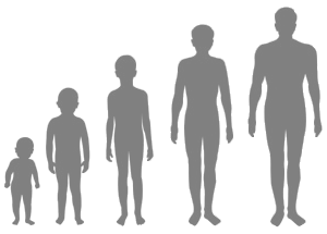
Figure 1: Proportionate growth in humans.

Growth and development of different structures in animals and plants has been a source of fascination and bewilderment for scientists and laymen alike. As a baby animal grows into an adult, it is often seen that different body parts in animals grow roughly at the same rate, keeping the overall shape approximately unchanged (see figure 1). This property is called proportionate growth. Of course, this is not exactly true, e.g., in humans, limbs grow faster than head, some physical changes appear at puberty, etc. However, proportionate growth provides a good starting description. We would like to argue that in spite of a lot of work in developmental biology for over a century, this basic phenomena in the problem of development is not well-understood.

The usual biological explanation of this would invoke different chemicals (hormones, growth factors…) that turn on and off the production of other chemicals according to the genetic master plan given in the animal’s DNA. But this approach, focussed on precise identification of chemical agents for various processes is not quite satisfactory. It is like saying in a murder mystery, “the knife did it”. We would like to look at this problem from a physicist’s perspective, and would like to construct simple physics models that show proportionate growth. Following the philosophy of d’Arcy Thompson [2], we would like to focus on the interplay of growth and geometrical structures, without getting bogged down in details of chemistry. The models we study are qualitatively different from other models of growth that have been studied by physicists in the past. Typical examples of growing structures that have been studied in physics so far are growth of crystals from a super-saturated solution, or diffusion limited aggregation, or viscous fingering, surface growth in molecular beam epitaxy. In all these cases, the growth occurs on the outer surface, and the inner parts once formed remain frozen. In fact, finding systems that show proportionate growth outside biology is rather difficult. This is because proportionate growth implies regulation, which requires some communication and long-range interaction between different parts of the body: this is not easily captured in the simpler processes mentioned above.

3 Self-organization and sandpiles

In the 1970’s, Haken, Nicolis, Prigogine and coworkers emphasized that an important characteristic of living systems is that they are ‘self-organized’ [3, 4]. Here ‘self-organized’ is not just an autonomous system, but a non-equilibrium steady state that has some internal self-regulation, and typically shows, amongst other things, self-generated complex spatial structures.

In 1987, Bak et alextended this idea of self-organization to other classes of natural systems out of equilibrium, like earthquakes and solar flares. They noted that these systems by their own natural dynamics tend to, and stay at, a critical state at the edge of stability, and called these Self-Organized Critical [5]. They proposed a simple model of sandpiles to illustrate this idea. A pile formed by dropping sand on a flat table is critical in the sense that the relaxation event of the system on the addition of a single grain (called an avalanche), has a wide distribution of sizes. This model has an interesting mathematical structure, and has inspired a large number of studies, of this, and other models of self-organized criticality [6, 7]. However, our interest in this paper is not in the criticality shown by the sandpile model at its steady state, but the self-organization shown in the interesting pattern that are generated in growing sandpiles. We hope that study of growing patterns generated in the sandpile model will also help in a better understanding of the original questions that led to its study.

We will show in this paper that the abelian sandpile model provides a very interesting model of pattern formation and proportionate growth. It is analytically tractable, and at least in some simpler cases, the asymptotic patterns can be fully characterized. It thus adds to the small number of known analytically tractable complex systems with simple rules.

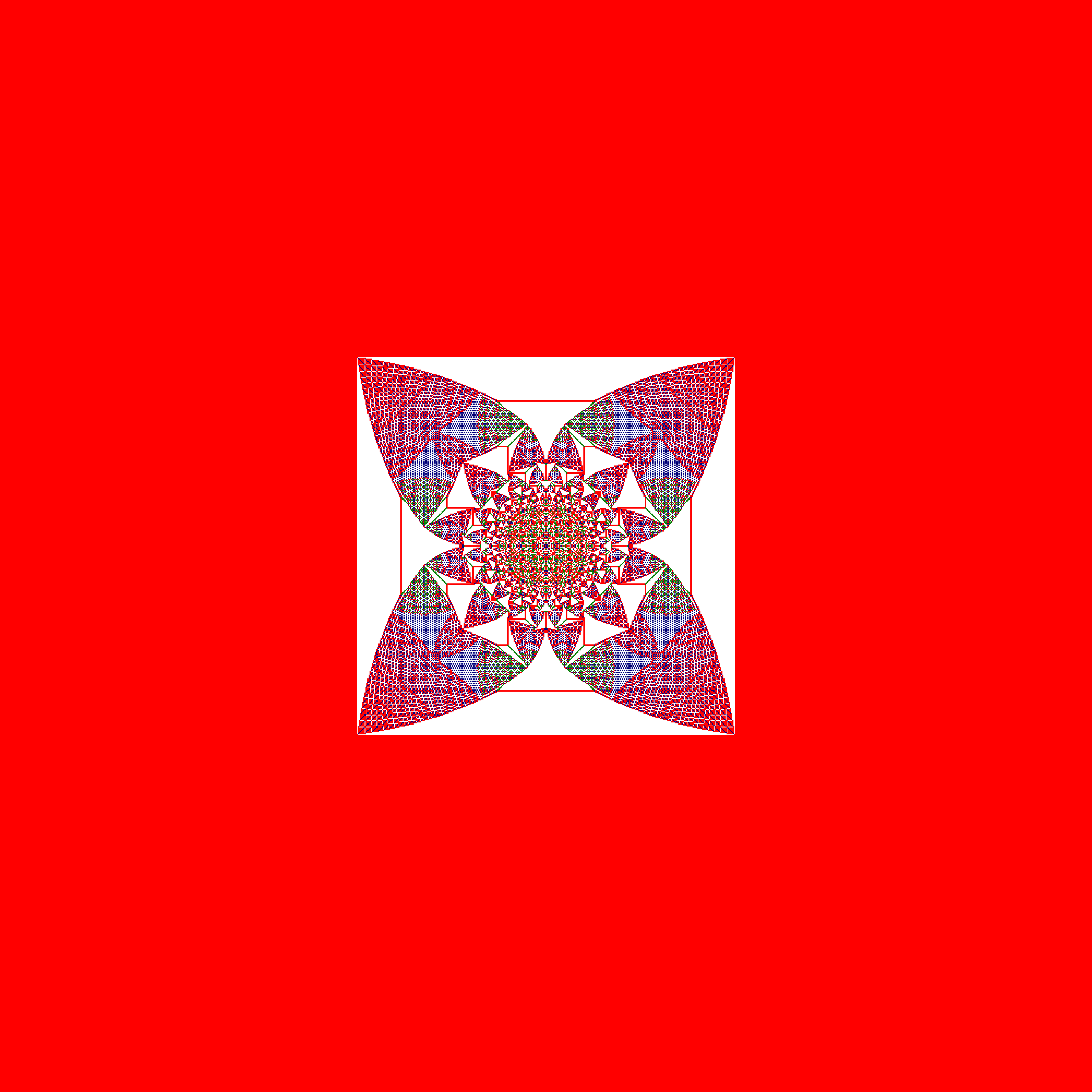
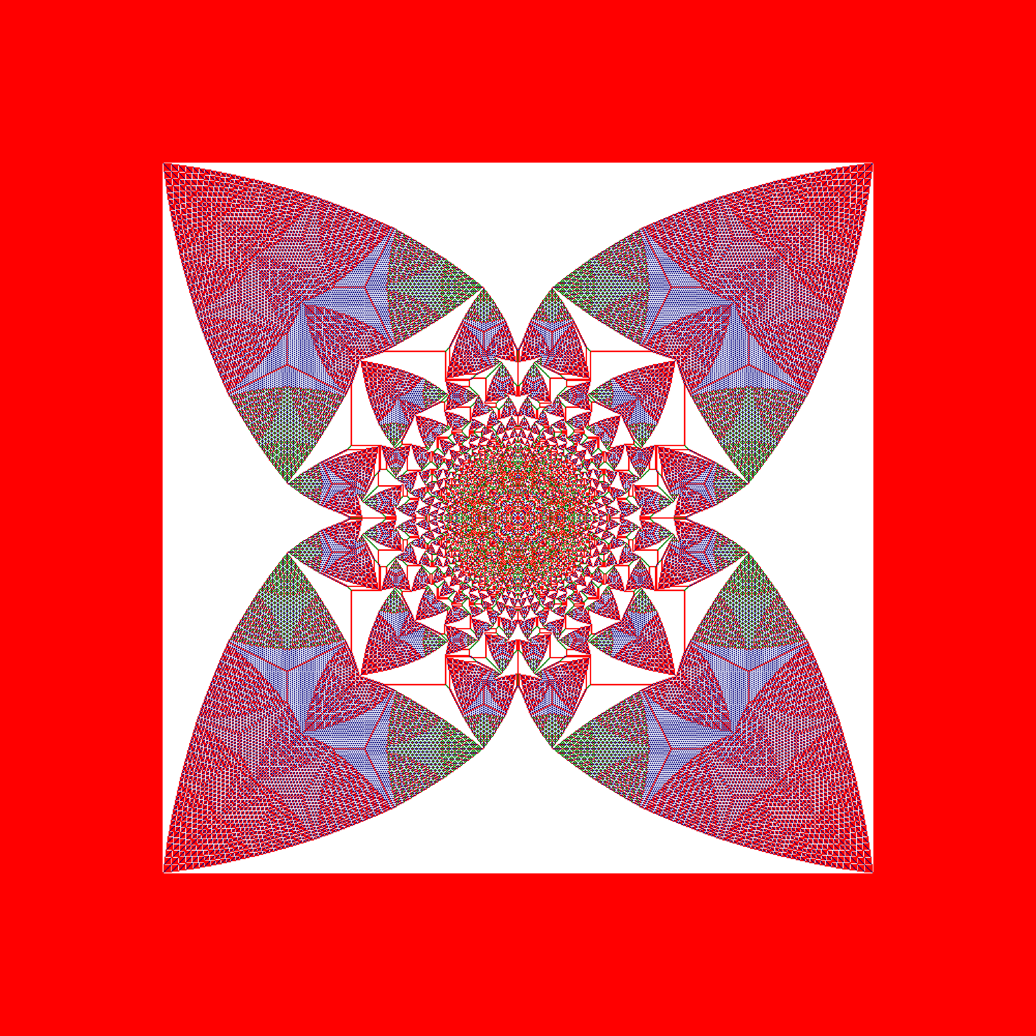
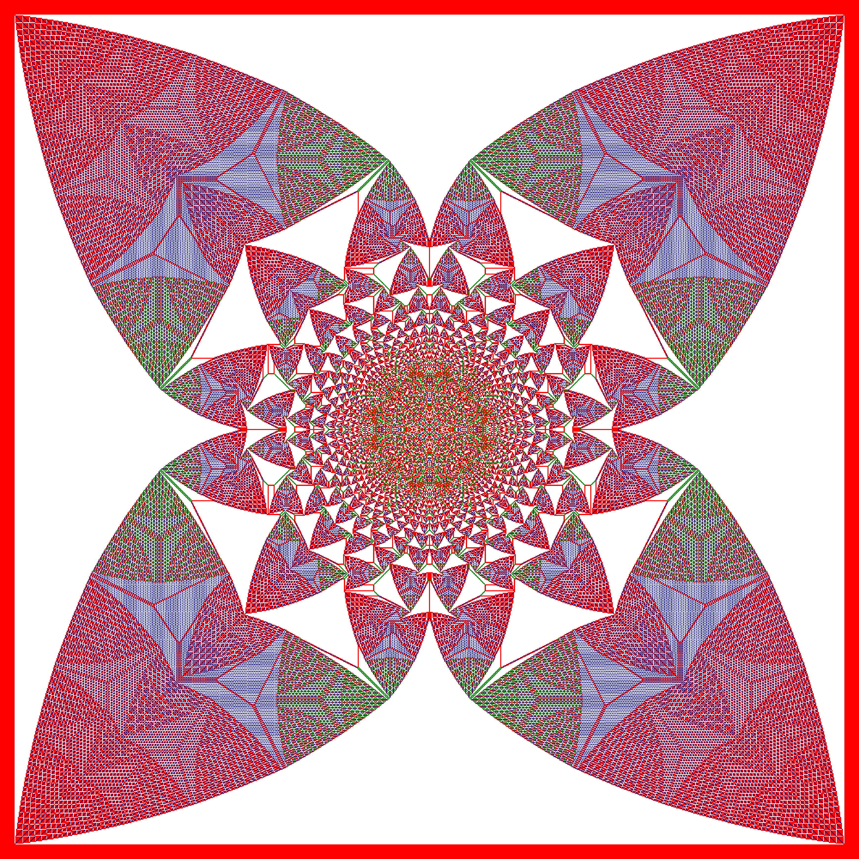
Figure 2: Patterns formed on a square lattice with initial height 2 at all sites for $N=4\times 10^{4}$, $2\times 10^{5}$, and $4\times 10^{5}$. Color code: $0,1,2,3=$ B, G, R, W. The patterns are on the same scale. Zoom in for details in the electronic version. Figures reproduced from [1].

     

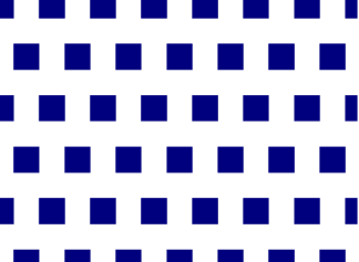
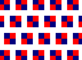
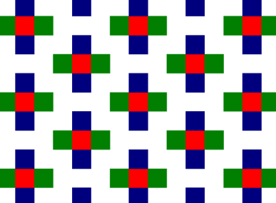
Figure 3: Some examples of periodic patterns in heights in figure 2, obtained by zooming into different patches. Color code same as in the original figure. Figures reproduced from [1].

4 Definition of the model

To make a primitive and simple model of biological growth, we note only some basic facts from biology. The first is that food is required for growth. Intake of food is typically from a localized organ (the ‘mouth’), and the nutrients are then transported to all parts of the body. The second is that the basic process in biological growth is cell-division. This is a threshold process in the sense that a cell will not divide if it does not have enough nutrients. And the third is that same food becomes different tissues in different parts of the body.

A well-studied model of threshold dynamics is the Abelian Sandpile Model [5, 8]. For simplicity, we define it on a square lattice. At each site $i$ there is a non-negative integer height variable $z_{i}$, which is called the number of sand grains at $i$. We say that a site is unstable, if the height at the site exceeds $3$. An unstable site relaxes by toppling: the height at the site is decreased by $4$, and the height at each neighboring site is increased by $1$. If this results in any of the neighbors becoming unstable, they are relaxed in the same way, until all sites are stable.

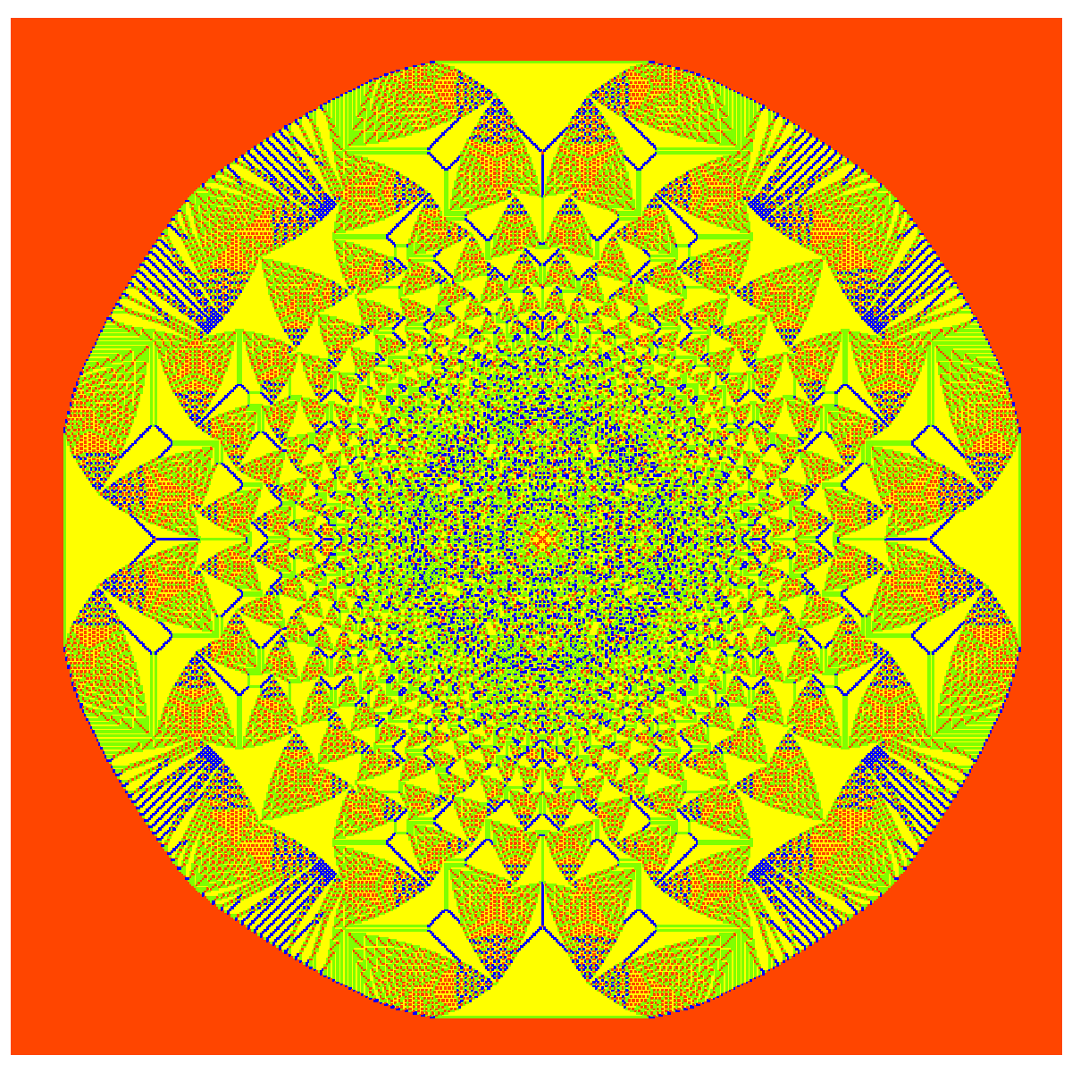
Figure 4: Pattern produced by adding $N=4\times 10^{5}$ particles at the origin, on a square lattice ASM, with initial state of all height $0$. Color code: $0$, $1$, $2$, $3=$ R, B, G, Y. Zoom in for details in the electronic version.

We start with a periodic stable configuration of heights on an infinite lattice. Then, we add one grain at the origin, and relax the configuration, if unstable. Then add another grain, and relax. And so on.

This model has the property that if a configuration has several unstable sites, the order in which they are relaxed does not matter. The operations of adding particles at different sites and relaxing commute with each other. The operators form an abelian group, and hence this model is called the abelian sandpile model. The pattern obtained after $N$ grains have been added is a deterministic pattern. For different starting backgrounds, one gets different patterns.

In figure 2, we have shown the patterns corresponding to three different values of $N$, starting with a background with all sites with height $2$. We see that the pattern for larger $N$ is bigger, but has a similar structure: it shows proportionate growth. It is important to note that as pattern grows, structures at finer length scale are formed near the origin. Once formed, they grow proportionately and move away from origin.

The pattern in figure 2 consists of distinct structures, called patches here, with sharp boundaries. The very interesting and unexpected observation is that within a patch, the arrangement of heights forms a perfectly periodic structure, with only a few ‘defect lines’. Some examples of the periodic structures are shown in figure 3. When $N$ is increased, the sizes of the patches increase, and their location on the lattice will also change. The whole pattern consists of these periodic patches sewn together into a quilt-like whole.

One can similarly define the sandpile model on other lattices, and study patterns in other backgrounds. In higher dimensions also, we see the same phenomena, but we will confine our discussion here mostly to two dimensions, for ease of display. In figure 4, we show the pattern on the square lattice, when the background is all sites having height zero. In this case also, we see proportionate growth.

In figure 5(a), we show the graph defining the F-lattice. This is a directed square lattice with two arrows in and two arrows out at each vertex. The sandpile model on this graph is defined by the rule that any site with number of grains $\geq 2$ is unstable, and topples by sending two grains along the outward arrows. If we start with a checkerboard background with alternate sites having $1$ and $0$, and then add $N$ grains at the origin, the resultant pattern is shown in figure 5(b). In particular, we note here that the asymptotic pattern shows an eight-fold rotational symmetry, higher than the symmetry of the underlying lattice.

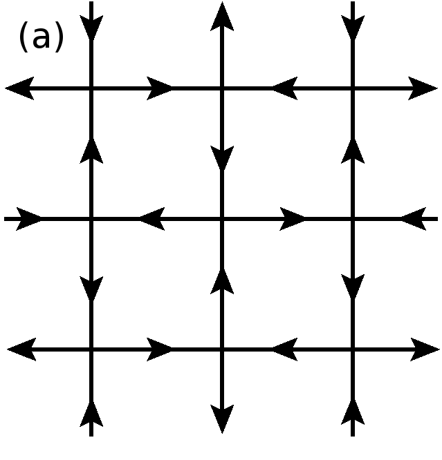
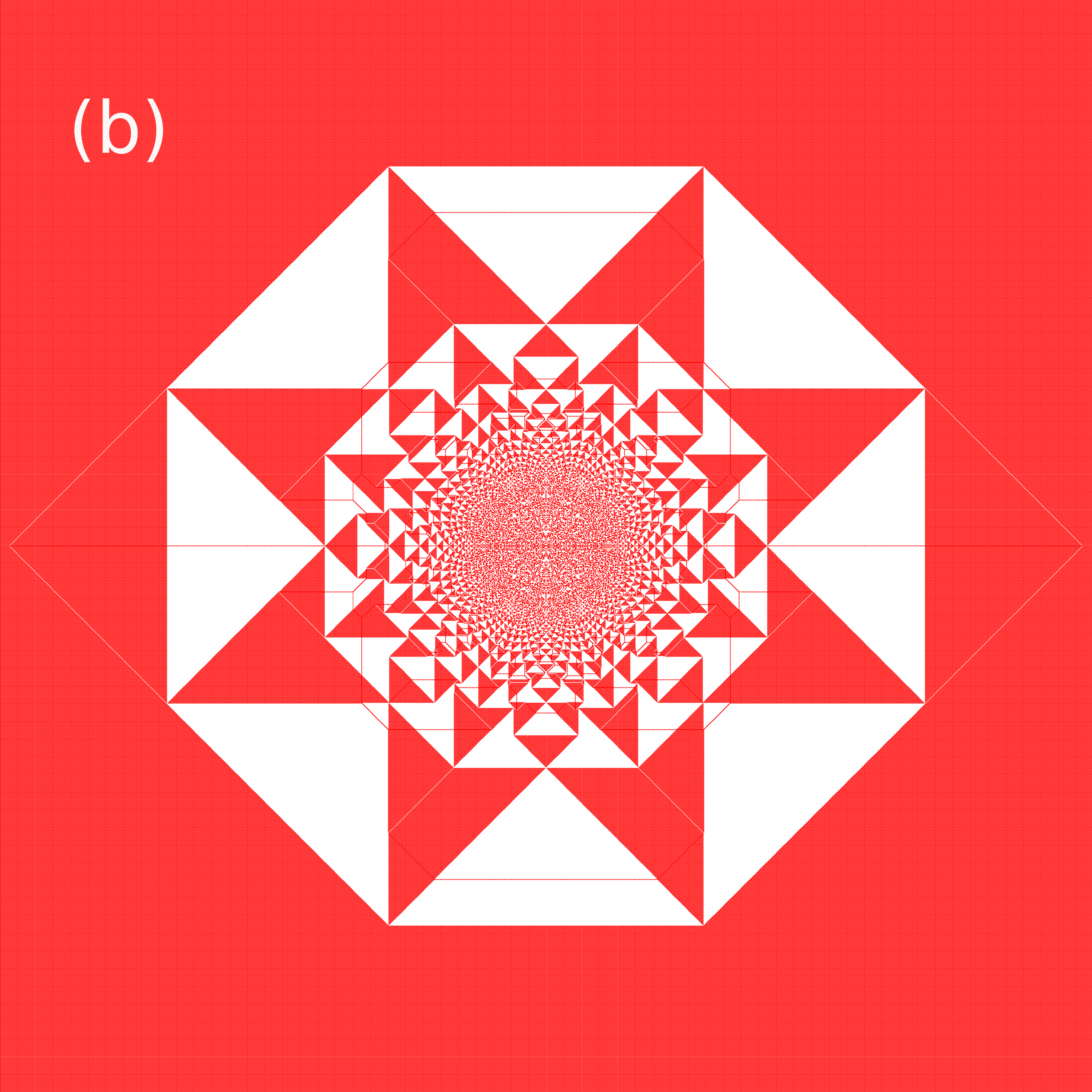
Figure 5: (a) The F-lattice, with two in-arrows and two out-arrows at each vertex of a square lattice. (b) The pattern produced by adding $2\times 10^{5}$ particles at the origin, on the F-lattice with initial background being checkerboard. Color code: $0=$ red, $1=$ white. The apparent red coloured patch is actually a checkerboard arrangement of red and white. Zoom in for details in the electronic version.

Patterns produced in sandpile models have been studied almost as long as sandpiles themselves. Liu et al[9] noted that patterns produced by relaxing special unstable states in the abelian sandpile model have complex fractal-like internal structures. First studies dealt with the shape of the boundary of the toppled cluster in a centrally seeded sandpile [10]. Bounds on the rate of growth of these boundaries were obtained in [11] and subsequently improved by [12, 13]. First detailed study of the periodic structures in the pattern was by Ostojic [14]. He also noted the piece-wise quadratic nature of the toppling functions within a patch. The first pattern to be characterized fully was a sandpile pattern on the F lattice [15]. In this case, the asyptotic pattern was determined in terms of the solution of the Laplace equation on the adjacency graph of the pattern. This technique was subsequently used in [16] to characterize patterns with more than one site of addition and also those produced in presence of absorbing sites. The effect of external noise on the pattern were studied in [17]. We have not been able to characterize fully the pattern on the square lattice in a similar way. In this case when the background is with all heights zero, the existence of a limit pattern has been proved rigorously [18].

There are other spatial patterns formed in the sandpile model, like the identity [11, 19] or the configurations produced by relaxing from a uniform unstable state [9]. These also show complex self-similar structures which are similar to those studied in this paper [20].

Growing complex patterns has also been studied in other models, similar to the sandpile model. For example, in the Internal Diffusion Limited Aggregation model [21] it has been shown that the boundary of the asymptotic pattern is related to the classical Stefan problem in hydrodynamics [22]. Levine and Peres have proved the existence of a limit shape for the pattern with multiple sources [23]. There are several other studies on patterns in Eulerian walkers [24, 25, 26, 27], infinitely divisible sandpiles and non-Abelian sandpiles [28].

5 General scaling theory for the asymptotic patterns

Let us denote the diameter of the pattern for a given value of $N$ by $\Lambda$. We define a reduced coordinate $\vec{r}\equiv(x,y)=\vec{R}/\Lambda\equiv(X/\Lambda,Y/\Lambda)$. Let $T_{N}(\vec{R})$ be the number of topplings at point $\vec{R}$. Then, the property of proportionate growth may be stated in terms of the scaling of $T_{N}(\vec{R})$ with $N$, or equivalently, with $\Lambda$. If the pattern shows proportionate growth, then, up to an overall multiplicative constant, the leading behavior of $T_{N}$ depends only on the reduced coordinates $\vec{r}$:

$$T_{N}(\vec{R})\sim\Lambda^{a}\phi(\vec{R}/\Lambda).$$ (1)

In addition, we expect that $\Lambda\sim N^{1/b}$, where $a$ and $b$ are some exponents. More formally, we define the function $\phi(\vec{r})$ by the equation

$$\phi(x,y)=\lim_{\Lambda\rightarrow\infty}\Lambda^{-a}T_{N}(\lfloor\Lambda x\rfloor,\lfloor\Lambda y\rfloor),$$ (2)

where $\lfloor x\rfloor$ is the largest integer less than or equal to $x$. If this limit exists, with a non-trivial function $\phi(\vec{r})$, then the pattern shows proportionate growth.

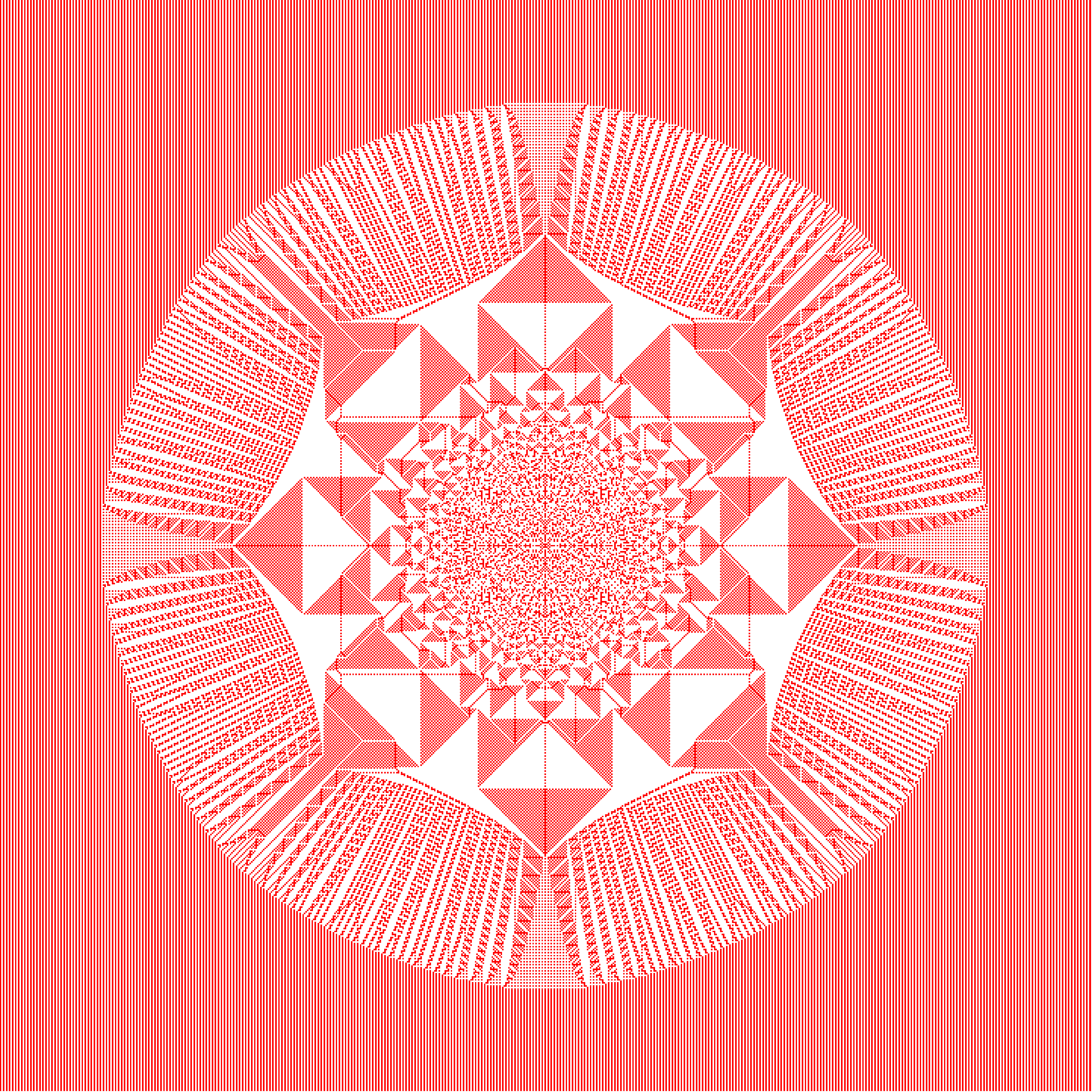
Figure 6: An example of a pattern with patches with aperiodic structures. This is produced by adding $N=10^{4}$ particles at the origin, on the F-lattice ASM, with initial state of alternating columns of $1$’s and $0$’s. Color code: red $=0$, white $=1$. Zoom in for details in the electronic version.

We note that lattice laplacian of $T_{N}(X,Y)$ gives the local change in height, and hence specifies the asymptotic height pattern. The function $\nabla^{2}\phi(x,y)$ gives the local density of excess particles in the neighborhood of a point corresponding to the reduced coordinate $(x,y)$. The excess number of grains per site is bounded everywhere. This implies that

$$a\leq 2.$$ (3)

Our analysis of the sandpile patterns depends on the following remarkable theorem: in each patch with a periodic height pattern, we can only have $a=2$ or $a=1$. In addition, within a periodic patch, $\phi(x,y)$ is a polynomial function of $x$ and $y$ of degree $a$.

The proof depends on the fact that $T_{N}(X,Y)$ is an integer function of integer arguments $X$ and $Y$, and any higher order terms in the Taylor expansion of $\phi(\vec{r})$ are not consistent with this condition. For example, a cubic term of the form $K(\Delta x)^{3}$ in the Taylor expansion of $\phi(x_{0}+\Delta x,y_{0}+\Delta y)$ can only come from a term of the form $K(\Delta X)^{3}/\Lambda^{3-a}$ in the expansion of $T_{N}$. But given that $\Delta X$ and $T_{N}$ are both integers, this would require defect lines with a spacing of order $\Lambda^{1-a/3}$. Since a periodic patch which itself has diameter of order $\Lambda$, by definition, does not have any defect structures having this intermediate scale of length, we conclude that $K=0$. Similar argument holds for other cubic, or higher order terms in the Taylor expansion. For details, see [29].

Sometimes, the generated patterns does show a large number of defect lines. Examples are the patterns in figure 4 and figure 6. The latter pattern is generated on the F-lattice, when the initial background consisted of alternate columns of 1’s and zeroes. The inner part of the pattern consists of periodic patches, where each patch occupies a non-zero fraction of the area of the pattern. However, in the outer rim, we see a large number of radial defect lines. Thus, for this pattern, it would appear that the function $\phi(\vec{r})$ is a piece-wise quadratic function of $\vec{r}$ in the periodic patches, except in the outer rim region. Of course, it may be that the outer rim region, is not a single large patch, but a union of many periodic patches.

Interestingly, the value of the exponent $b$ is much less constrained, and we can get different values of $b$, with $b\leq d$ ($d$ is the dimension of the lattice), depending on the initial periodic background chosen.

If the density of particles is low enough, then one gets a pattern where $\Lambda\sim N^{1/d}$, where $d$ is the dimension of the lattice. For example, for the $d$-dimensional hypercubic lattice, if all sites in the initial pattern have heights $\leq(2d-2)$, where the threshold height is $2d$, then the pattern has $\Lambda\sim N^{1/d}$. If on the other hand, sufficiently many sites have height $(2d-1)$, e.g., if they form a spanning cluster, then clearly, we get infinite avalanches, and $\Lambda$ is infinite for finite $N$.

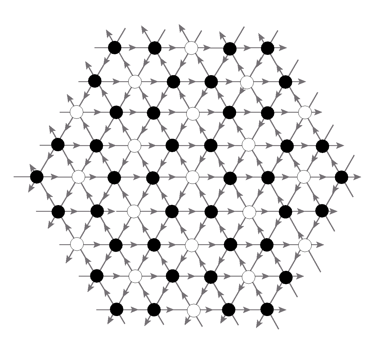
(a)

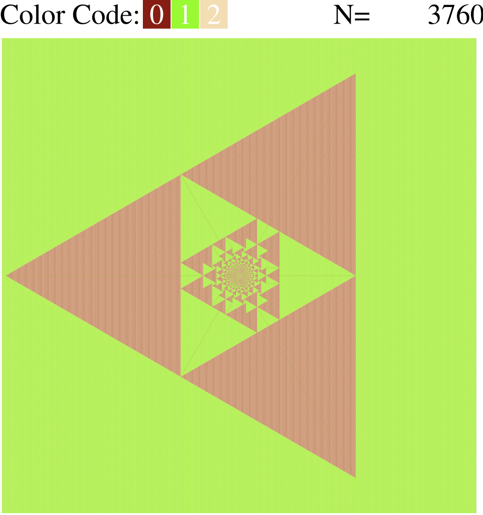
(b)

Figure 7: (a) Directed triangular lattice. In the background configuration, filled and unfilled circles denote $z=1$ and $2$. (b) The pattern produced on the background by adding $N=3760$ particles. The apparent green patch denotes background height configuration. Zoom in for details in the electronic version. Reproduced from [29].

In figure 7, we have shown a directed triangular lattice, with three arrows in, and three out of each vertex. The toppling rule for the sandpile is that any site with more than $2$ grains is unstable, and transfers one grain each in the direction of outgoing arrows. Starting with the background shown in figure 7(a), the pattern generated by adding grains and relaxing is shown in figure 7(b). In this case, $\Lambda\sim N$, and $b=1$. In [29], we have discussed an infinite family of initial backgrounds on this lattice that all give $b=1$.

More interestingly, on the F-lattice, we found a family of initial backgrounds that gives $b$ which lies between $2$ and $1$. In figure 8 we show the periodic background on the F-lattice, and the generated pattern. When $b<d$, the mean excess density in the patch in the asymptotic pattern is zero. In this case, the density inside the patches is same as in the background, and added particles sit on the boundaries of patches. Some boundaries can also have a deficit of particles. We have shown only the boundaries of the patches. We will refer to this pattern as the ‘bat-pattern’. Our numerical studies [29] have found that the wing-span of this bat varies as $N^{b}$, with $b\approx 0.55$. However, one also sees some region with non-zero excess areal charge density in the pattern (solid colour in the figure). The boundaries of these solid coloured regions seem to be exact parabolas, and so the width of these regions would have to scale as $\Lambda^{1/2}$. This implies that these solid coloured regions will shrink to two vertical lines in the asymptotic pattern. The potential function would not be continuous along these lines.

There are also other periodic backgrounds on the F-lattice, for which we found other values of $b$. The general shape is similar to that of the bat-pattern. For details, see [29].

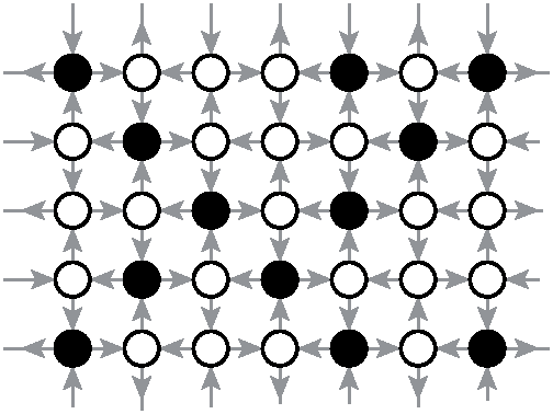
(a)

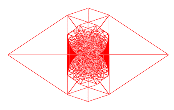
(b)

Figure 8: The ‘bat-pattern’: (a) the unit cell of the periodic initial pattern, and (b) the pattern generated. Only the boundaries of patches are shown.

6 Exact characterization of the patterns

It is not immediately obvious how one can characterize these complex patterns in detail. The first level of description is clearly structural. One describes the patterns by describing which periodic patterns are found in which patch, and which patch is adjacent to which. Formally, we define an adjacency graph for the pattern, where the vertices are patches, and then we draw a link between two vertices if they are adjacent. The pattern is described by giving its adjacency graph, and the periodic pattern associated to each vertex. The next level of description gives the metric properties of the patches: their position and exact equations of the boundaries, etc.

For the patterns that we have been able to characterize, we construct the adjacency graph by looking at the pattern. It is easy to see the adjacency relation between the larger patches. But the patches become smaller and more numerous as we go closer to the origin, and they are not clearly resolved. In this case, we extrapolate that the observed regularity of structure will continue to hold at higher resolutions.

The procedure is best illustrated by an example. To characterize the pattern in figure 7, we note that in this case $a=1$, and hence the potential function is piece-wise linear.

1. In a particular patch, say denoted by $P$, we will express the piece-wise linear function $\phi(x,y)$ as

   $$\phi_{P}(x,y)=a_{P}x+b_{P}y+c_{P}.$$ (4)

   Here $a_{P},b_{P}$ and $c_{P}$ are parameters that may be used to specify the patch. Since $T_{N}$ has to be an integer function, this implies that $a_{p}$ and $b_{p}$ are rational numbers. Different patches may then be represented as points in a two-dimensional plane with Euclidean coordinates $(a,b)$. By actually examining the values of these parameters for several patches, we noticed that the allowed values of $(a_{P},b_{P})$ form a hexagonal lattice in this space, and patches corresponding to nearest neighbour vertices on this lattice are adjacent patches in the original pattern. In addition there are some additional adjacencies for patches lying along the six symmetry directions in the original pattern. Thus, each patch may be labelled by two integers $(\ell,m)$, which give the coordinates on the hexagonal lattice.

2. The potential $\phi(x,y)$ is a continuous function of its arguments. Then, the equation of the boundary between two adjacent patches $P$ and $P^{\prime}$ is obtained by the condition that $\phi_{P}=\phi_{P^{\prime}}$ along the boundary. From the linearity of $\phi_{P}$ and $\phi_{P^{\prime}}$, it follows that all boundaries are straight lines.

3. The condition that three patches $P,P^{\prime}$ and $P^{\prime\prime}$ meet at a point implies a condition on the coefficients $c_{P},c_{P^{\prime}}$ and $c_{P^{\prime\prime}}$. It is easy to check that this condition implies that $c_{P}$ satisfies a Laplace equation on the hexagonal lattice in the adjacency graph (leaving out the extra edges in the graph that are not nearest neighbor edges on the hexagonal lattice).

4. By solving the Laplace’s equation on the infinite hexagonal lattice, we determine all the $c_{P}$’s.

Once the potential in all the patches is determined, we can find the position of all patch boundaries, and the reduced coordinates of all corners of patches in the asymptotic pattern are determined exactly. For example, in this case, we find that the equation of the right boundary of the triangle formed is $x=1/3$. Other backgrounds with similar adjacency structure, but slightly different relative sizes of patches are discussed in [29].

For the patterns with $a=2$, the potential is a quadratic function in each patch. The pattern in figure 5 is one such example. The adjacency graph has the structure of a square grid on a two-sheeted Riemann surface. One needs six coefficients to specify the quadratic function in each patch. Out of these, the three coefficients of the quadratic terms are specified in terms of the integer coordinates $(l,m)$ of the patch on the adjacency graph. The coefficients of the linear term in $x$ and $y$ again are found to satisfy the Laplace equation, and hence the solutions are determined in terms of lattice Green function for the square grid on a two-sheeted Riemann surface. For details, see [15].

7 Effect of noise

Clearly, deterministic cellular automaton models are not very realistic model of biological growth, as real growth involves a fair amount of noise. We have studied the effect of noise in several ways [17].

If the point where particles are added is random, but lies in a box of size $n$, then when the diameter of the pattern is much bigger than $n$, the input acts like a point source, and the asymptotic pattern is unchanged. If the region where particles are added is a small region near the origin, but this region also grows proportionately with the pattern, the intricate substructures of patches in this small region is washed out, but the outer larger patches have the same appearance.

We also studied the effect of boundaries on the growing pattern. We considered growth in a half-space, where only the points $(x,y)$ with $y\geq 0$ are available for growth, and the point of addition is the origin. Any particle that is transferred to a site outside the lattice is lost. In this case, a straight forward analysis using the lattice propagator in the presence of a boundary shows that the diameter of the pattern grows as $N^{1/3}$. More generally, if the growth occurs in a wedge of angle $\theta$, the diameter of the pattern grows as $N^{\frac{\theta}{2\pi+\theta}}$.

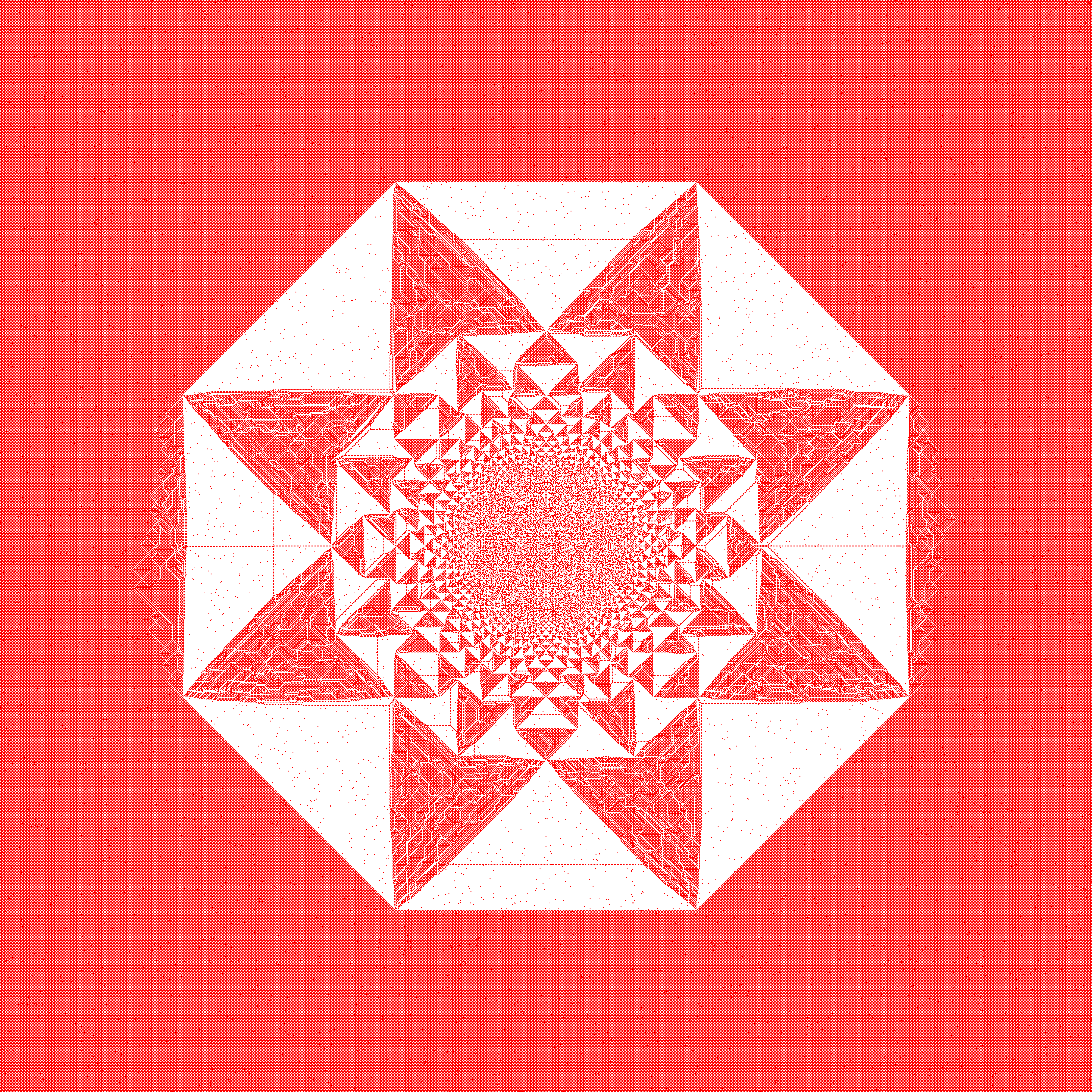
Figure 9: Pattern grown on the F-lattice with noisy checkerboard background where some of the heights $1$ are replaced by $0$’s. (a) $1\%$ sites changed, with $N=228\times 10^{3}$, and (b) $10\%$ changed, with $N=896\times 10^{3}$. Color code: $0=$ red and $1=$ white. Zoom in for details in the electronic version. Reproduced from [17].

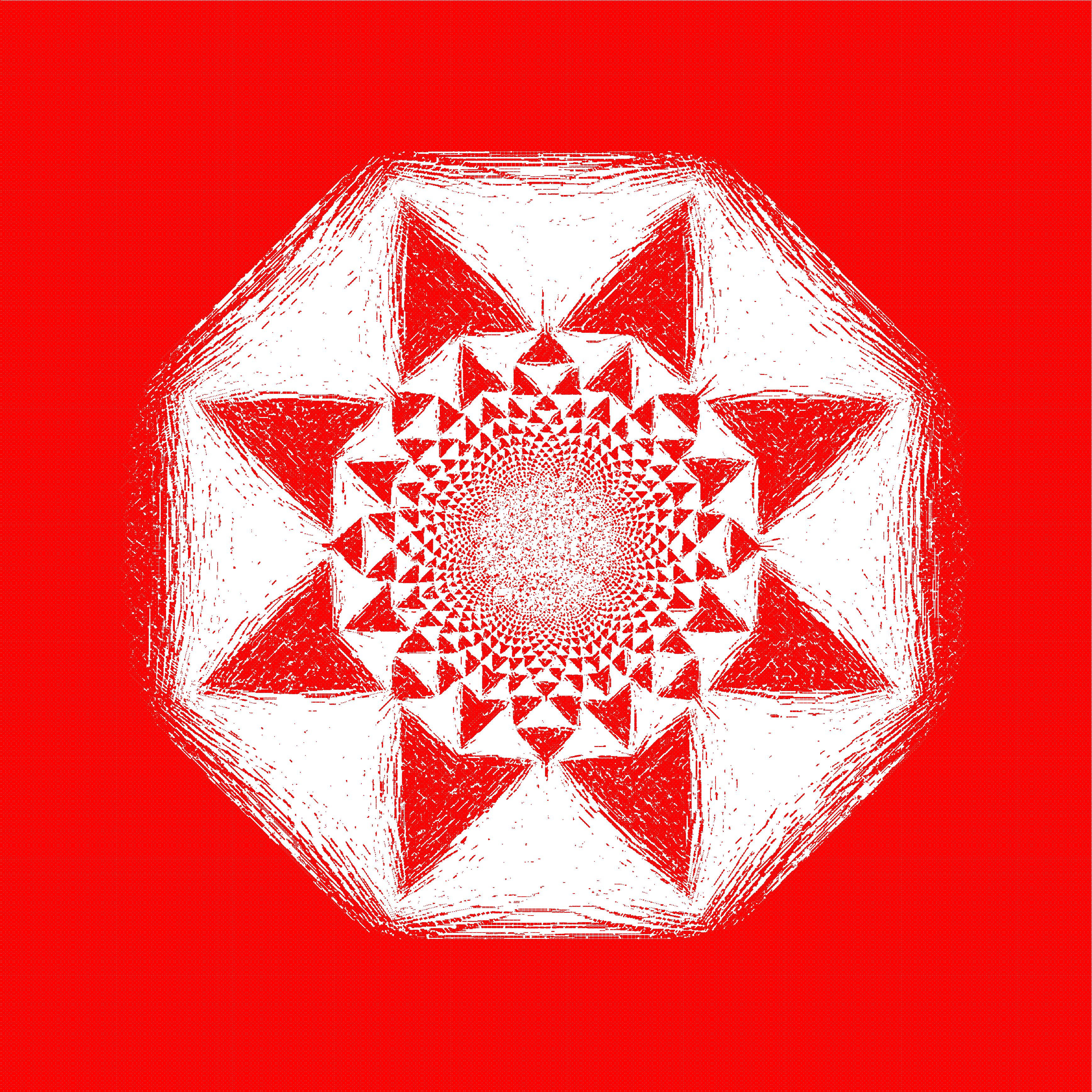
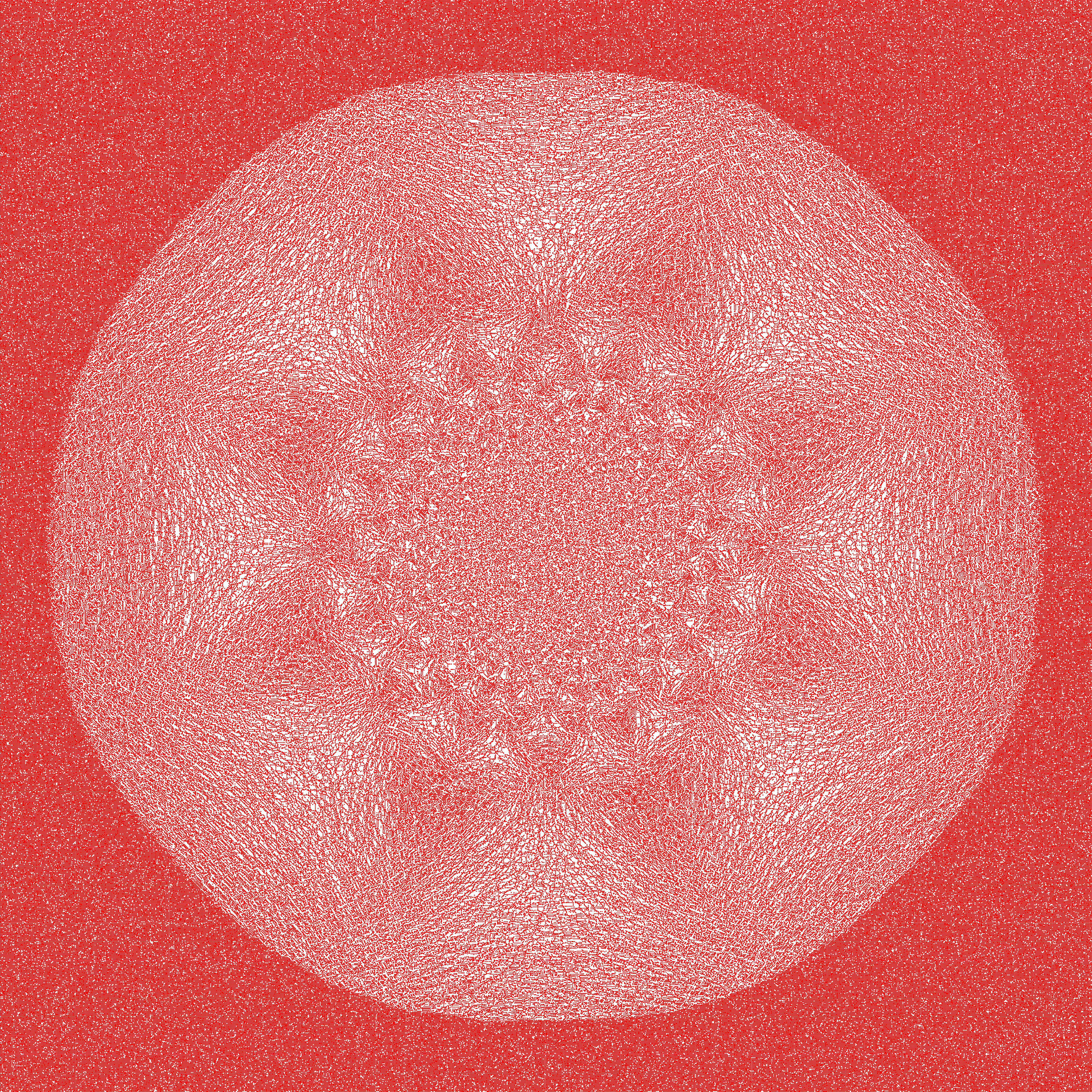
Figure 10: Pattern generated on the F-lattice with noisy checkerboard background where some heights are flipped. (a) $1\%$ sites changed (b) $10\%$ sites changed. For both patterns $N=57\times 10^{3}$. Color code: $0=$ red and $1=$ white. Zoom in for details in the electronic version. Reproduced from [17].

We also studied the problem when the initial starting background pattern is not a perfectly periodic pattern. For the octagonal pattern on the F-lattice, we studied the case when the initial configuration is the checkerboard pattern, with a small fraction of $1$’s randomly replaced by zeroes. The resulting patterns are shown in figure 9 for two different values of the noise strength. We find that one still gets a nontrivial pattern showing proportionate growth. For small noise-strength, this pattern appears to be a small deformation of the pattern without noise. The existence of sharp boundaries is quite surprising, as in the presence of noise, the potential function is no longer piece-wise quadratic. Since one can still define distinct patches in this case, we can also form their adjacency graph, which does not depend on the noise strength [17].

If we take the F-Lattice checkerboard background as the starting point, and to add noise, we flip the height of a small fraction of sites at random, changing height $1$ to zero, and also change $0$ to $1$, the resulting pattern is shown in figure 10, for two different strengths of the noise. We still see proportionate growth, with the asymptotic pattern showing the basic structure as the pattern without noise. However, now, there are no sharp boundaries between patches of low- and high-densities. There is an inhomogeneous density profile of particles in the asymptotic pattern, and this profile grows proportionately. The amplitude of the ripple in the density pattern decreases as the noise strength is increased.

At higher noise levels, the density-inhomogeneity in the pattern is not immediately visible with naked eyes, as may be seen in Fig. 11. Here in figure 11(a), we have shown the pattern formed with one particular realization of noise. However, if one forms several such patterns (with different realizations of noise in the initial background), and determines the mean change in density of particles, one can clearly see the nontrivial density profile in the pattern [ Fig. 11 (b)].

The very weak density inhomogeneity is reminiscent of convection patterns in the Raleigh-Benard problem, near the onset of convection. However, the origin of instability in the density profile in this problem is not yet understood.

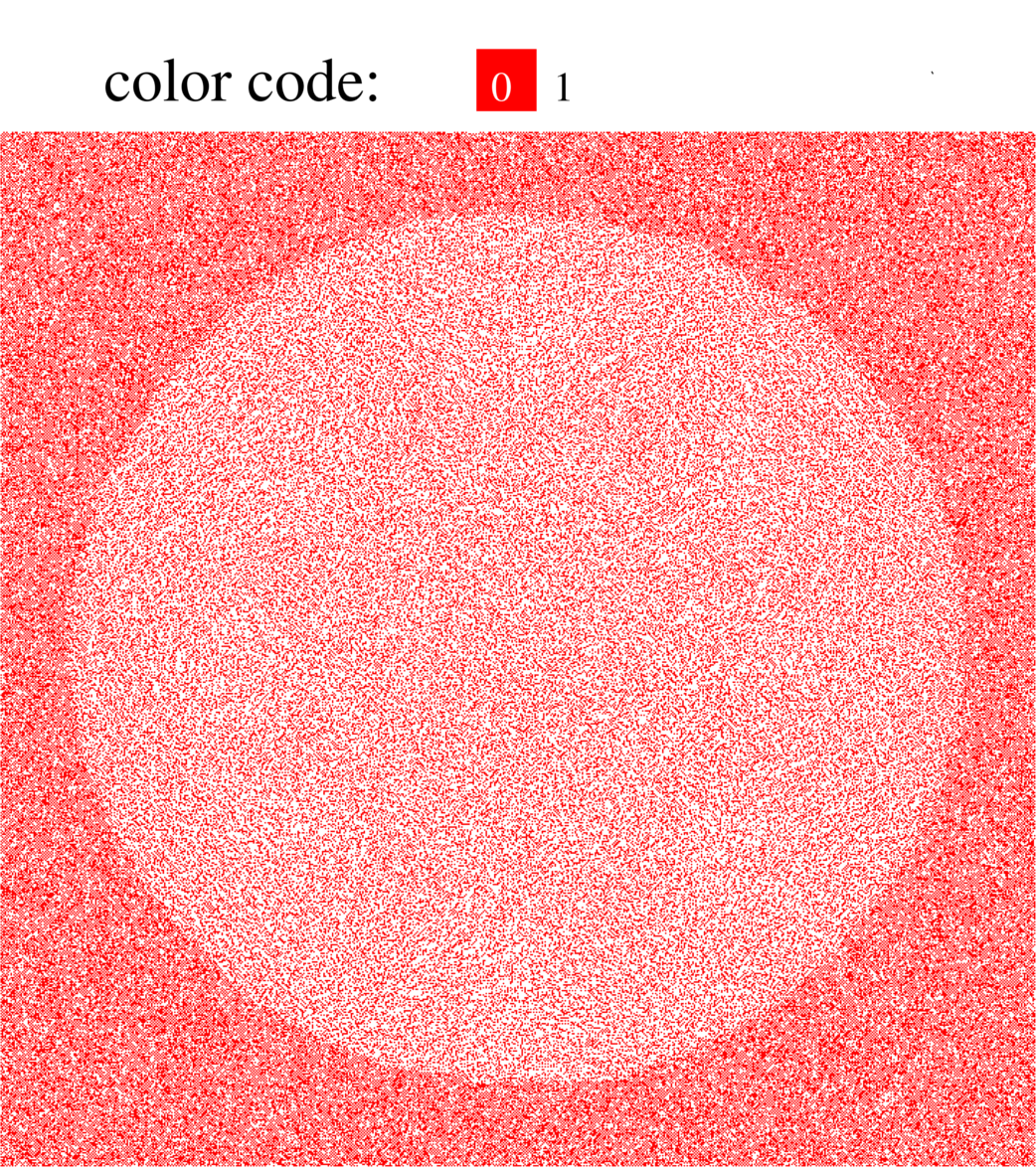
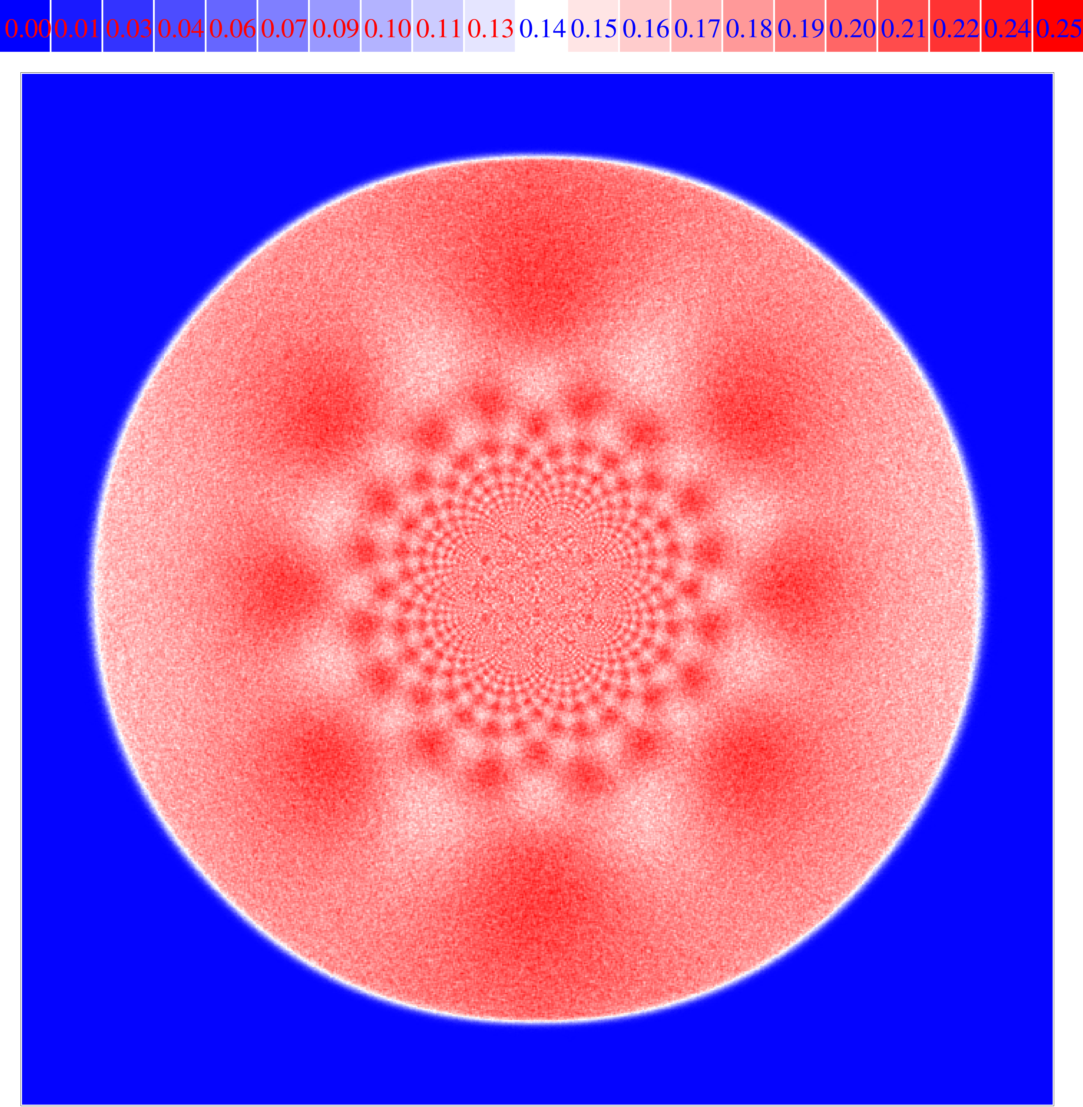
Figure 11: Pattern by adding $N=57\times 10^{3}$ particles on F-lattice, checkerboard background with $20\%$ sites flipped. (a) Pattern corresponding to a single realization of the noisy background. (b) The pattern in terms of difference in height from the background, averaged over $10^{5}$ realizations and also over the sublattice. Zoom in for details in the electronic version.

8 Other issues

If we allow dissipation in the topplings, then the growth tends to saturate. It is easy to see that the growth does not saturate exactly, and for deterministic toppling rules with dissipation, the diameter increases as $\log N$ [30]. If the dissipation is stochastic, and there is a small probability $\epsilon$ that a particle is lost per toppling, then the diameter still increases, but only as $\log N$ for $N\gg 1/\epsilon$. Also, while noise in toppling rules seems to wipe out the intricate details of the pattern without noise, some large scale features of the pattern, e.g. the non-circular outer boundary with some straight line-segments, seem to survive for $N\gg 1/\epsilon$. [30]

One can also study directed particle transfer rules. For example, we take a square lattice, with heights $\geq 3$ unstable, and particles are transferred in only along the north, south and east directions. The corresponding pattern is shown in figure 12. The basic unit of organization is not a periodic patch but a sliver made of aligned squares of slowly varying width. The pattern does not have proportionate growth, as different directions grow at different rate. Here, the transverse size along the $y$-axis grows as $\xi_{\perp}\sim N^{1/3}$, while the size along the growth direction $\xi_{\parallel}\sim N^{2/3}$.

In three dimensions, the pattern formed by similar directed transfer rules on a cubic lattice is shown in figure 13. Here the critical threshold is $5$, and on toppling, one particle is transferred along each neighbor except in the negative z-direction. We see that, in this pattern also, three distinctive head-thorax-abdomen type of features can be identified.

Because of the existence of two length scales, the arrangement of patches in these systems shows a more complicated structure. The typical size of a patch does not scale linearly with the diameter, and the fractional area of a patch in the asymptotic pattern is zero. Detailed characterization of such patterns has not been undertaken so far.

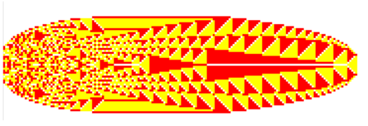
Figure 12: The ‘larva’ pattern formed with partially directed transfer rules on a square lattice with $N=10^{4}$ grains with initial background of all heights being zero. The color code used: $0=$ white, $1=$ red and $2=$ yellow.

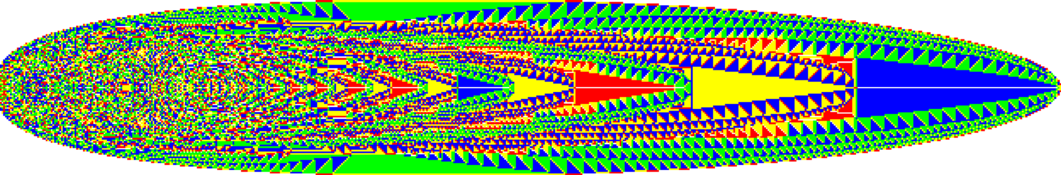
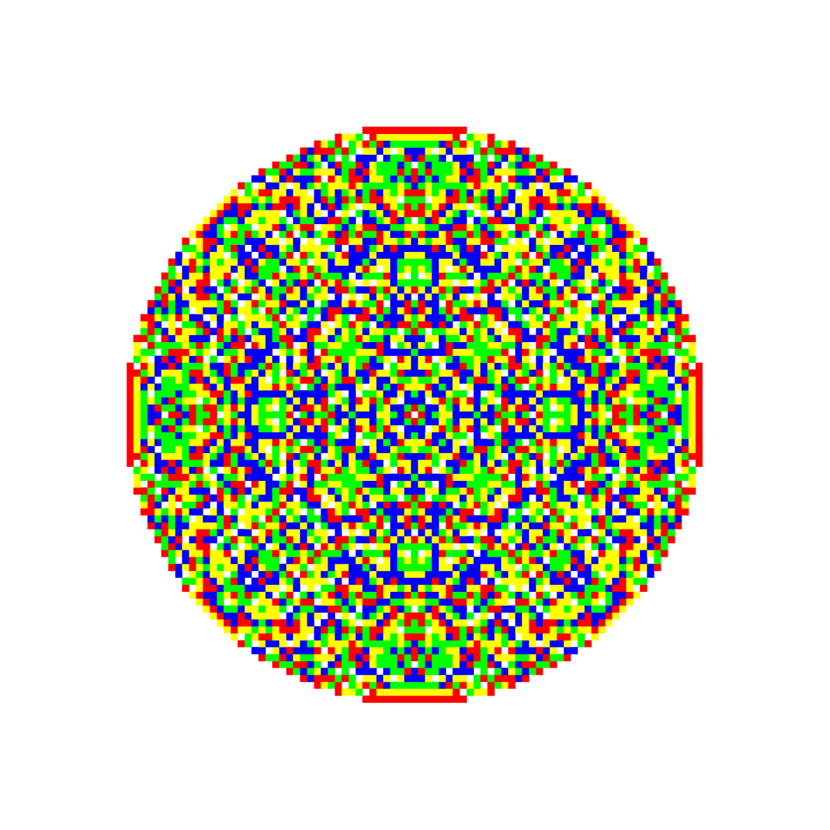
(a)

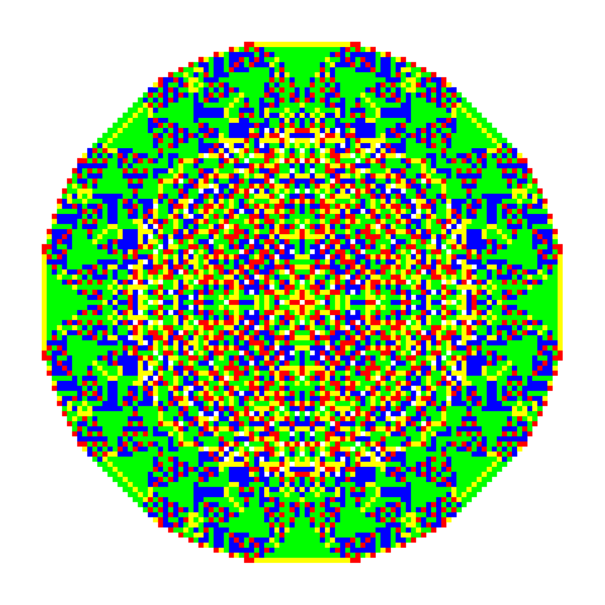
(b)

(c)

Figure 13: A three-dimensional ‘larva’ pattern formed on a directed cubic lattice. The pattern was obtained by adding $N=10^{7}$ grains on an initial background of all heights being zero. The particles were added at the central point of the left end. (a) shows the pattern on a plane dissecting the three dimensional pattern along the longitudinal direction. Here the colour code is $0=$ white, $1=$ red, $2=$ yellow, $3=$ blue and $4=$ green. The particles are added at central point the left end. (b)-(d) show cross sections perpendicular to the body axis at different positions indicated by the dotted lines in (a).

9 Concluding remarks

To summarize, we have argued that growing sandpile model generates interesting complex patterns, and shows proportionate growth using very simple evolution rules. They thus provide a simple mathematical model of this fascinating phenomena.

While we have mainly emphasized the property of proportionate growth, we would like to also note their importance for understanding morphogenesis. The classical model of morphogenesis is the Turing instability [31]. In this, one gets only a limited set of basic patterns with a small number of chemicals. Using the large choice of toppling rules, and starting backgrounds possible, the number of possible patterns that can be generated in abelian sandpiles is unlimited.

The most intriguing feature of these patterns is that these minimal models can sometimes produce patterns that have a striking similarity to the natural ones. For example, the patterns in figure 12 and figure 13 looks like a larva, with parts that look like the head, thorax, and the abdomen. There is no indication of these features in the toppling rules defining the pattern. In figure 14, we show a pattern generated on the F-lattice, using a background with unit cell made of tilted squares of side-length $\ell$. By varying $\ell$, we can get a flower-like pattern, and the petals of the flower become longer for larger $\ell$. The pattern shown was generated for $\ell=4$. One may have guessed the pattern would have bilateral symmetry, and petal-like structures, but the appearance of the anthers- and circular corolla- like structures is totally unexpected. Clearly, the model of sandpile toppling rules studied here is rather simplistic, but it is able to capture some crucial elements of the real, much more complicated phenomena.

(a)

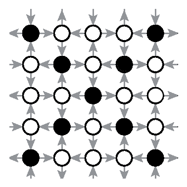
(b)

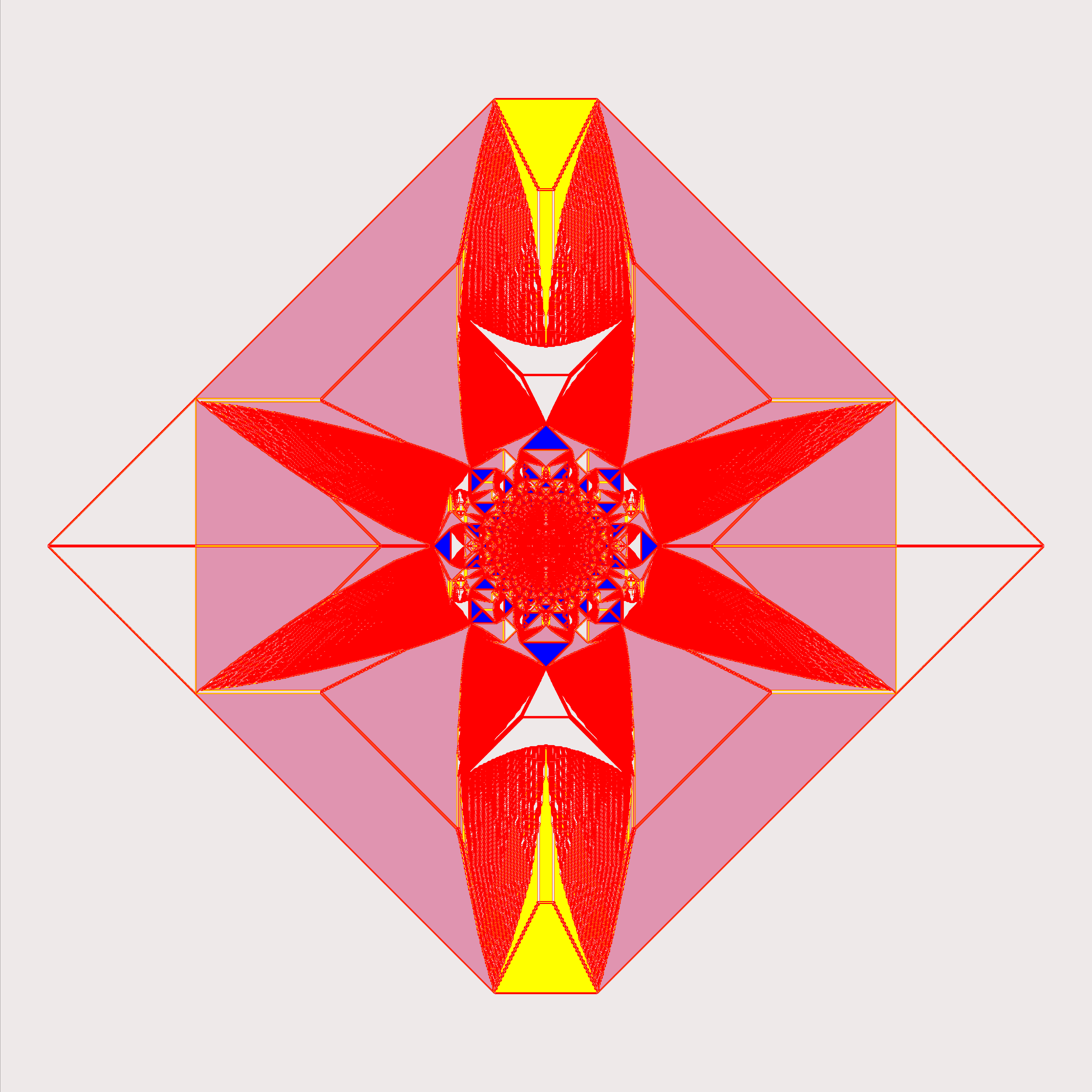
(c)

Figure 14: (a) A flower. (b) Unit cell of the background pattern with tilted squares on the F-lattice. The unfilled circles denote height $1$, whereas the filled ones represent empty sites. (c) The pattern produced by adding $N=256\times 10^{3}$ particles on the background. Different colours denote densities of particles, averaged over the unit cell of the background pattern. Zoom in for details in the electronic version.

Our motivations for our study of these patterns have been not only their beauty and fascinating diversity, but also the fact that they are analytically tractable. Our present understanding of this pattern-formation aspect of the problem is only partial. One has to take some important features of the patterns as experimentally seen. It is hard to derive these theoretically, directly from the definition of the problem. For example, in the F-lattice octagonal pattern of figure 5, we can determine the exact metric properties of the resulting pattern, by solving the Laplace’s equation on the adjacency graph of the pattern. But we have not been able to deduce the structure the adjacency graph, starting from the toppling rules.

There are many more complex patterns, for which the exact characterization seems more difficult, and would perhaps require some new approach. For fast-growing sandpiles, with the exponent $a=1$, it seems plausible that the mathematical techniques of tropical algebra [32] could be useful. Also, for the fractal patterns like the one shown in figure 8, the calculation of the fractal dimension is a challenging problem. There is an intriguing connection of the patterns generated here with the problem of Apollonian packing of circles [33]. The ‘pattern selection problem’ of predicting which patterns will be found for a given background, and given toppling rules is not understood at present. The variational formulation of this problem in terms of the ‘principle of least action’ seems to be a promising direction for further work [17]. Also, much more needs to be done to understand the pattern formation on noisy backgrounds.

References

References

- [1] T. Sadhu and D. Dhar. Modelling proportionate growth. Current Sci., 103(5):512–517, 2012.
- [2] D’Arcy W. Thompson. On growth and form. Cambridge :University Press, 1945.
- [3] G. Nicolis, I. Prigogine. Self-organization in nonequilibrium systems : from dissipative structures to order through fluctuations. A Wiley-Interscience Publication. J. Wiley and sons, 1977.
- [4] H. Haken. Information and Self-Organization: A Macroscopic Approach to Complex Systems. Springer Series in Synergetics. Springer-Verlag, 2000.
- [5] P. Bak, C. Tang, and K. Wiesenfeld. Self-organized criticality: An explanation of the 1/ f noise. Phys. Rev. Lett., 59:381–384, 1987.
- [6] P. Bak. How nature works: the science of self-organized criticality. Copernicus, 1996.
- [7] D. Dhar. Theoretical studies of self-organized criticality. Physica A, 369(1):29–70, 2006.
- [8] D. Dhar. Self-organized critical state of sandpile automaton models. Phys. Rev. Lett., 64:1613–1616, 1990.
- [9] S. H. Liu, T. Kaplan, and L. J. Gray. Geometry and dynamics of deterministic sand piles. Phys. Rev. A, 42(6):3207–3212, 1990.
- [10] D. Dhar. Studying Self-Organized Criticality with Exactly Solved Models. arXiv:cond-mat/9909009, 1999.
- [11] Y. Le Borgne and D. Rossin. On the identity of the sandpile group. Discrete Math., 256(3):775–790, 2002.
- [12] A. Fey and F. Redig. Limiting shapes for deterministic centrally seeded growth models. J. Stat. Phys., 130:579–597, 2008.
- [13] L. Levine and Y. Peres. Strong spherical asymptotics for rotor-router aggregation and the divisible sandpile. Potential Analysis, 30:1–27, 2009.
- [14] S. Ostojic. Patterns formed by addition of grains to only one site of an abelian sandpile. Physica A, 318(1):187 – 199, 2003.
- [15] D. Dhar, T. Sadhu, and S. Chandra. Pattern formation in growing sandpiles. EPL, 85(4):48002, 2009.
- [16] T. Sadhu and D. Dhar. Pattern formation in growing sandpiles with multiple sources or sinks. J. Stat. Phys., 138:815–837, 2010.
- [17] T. Sadhu and D. Dhar. The effect of noise on patterns formed by growing sandpiles. J. Stat. Mech., 2011(03):P03001, 2011.
- [18] W. Pegden and Smart C. K. Convergence of the abelian sandpile. Duke Math. J., 162(4):627 – 642, 2013.
- [19] M. Creutz. Abelian sandpiles. Comput. Phys., 5:198–203, 1991.
- [20] S. Caracciolo, G. Paoletti, and A. Sportiello. Explicit characterization of the identity configuration in an abelian sandpile model. J. Phys. A, 41(49):495003, 2008.
- [21] G.F. Lawler, M. Bramson, and D. Griffeath. Internal diffusion limited aggregation. Ann. Probab., 20(4):2117–2140, 1992.
- [22] J. Gravner and J. Quastel. Internal DLA and the stefan problem. Ann. Prob., 28(4):1528–1562, 2000.
- [23] L. Levine and Y. Peres. Scaling limits for internal aggregation models with multiple sources. J. d’Analyse Mathématique, 111(1):151–219, 2010.
- [24] V. B. Priezzhev, D. Dhar, A. Dhar, and S. Krishnamurthy. Eulerian walkers as a model of self-organized criticality. Phy. Rev. Lett., 77:5079–5082, 1996.
- [25] L. Levine and Y. Peres. Spherical asymptotics for the rotor-router model in . Indiana Univ. Math. J., 57:431–450, 2008.
- [26] A.E. Holroyd, L. Levine, K. Meszaros, Y. Peres, J. Propp, and D.B. Wilson. Chip-firing and rotor-routing on directed graphs. In In and Out of Equilibrium II, Progress in Probability, volume 60, 2008.
- [27] R. Dandekar and D. Dhar, in preparation.
- [28] A. Fey and H. Liu. Limiting shapes for a non-abelian sandpile growth model and related cellular automata. J. Cellular Automata, 6:353–383, 2011.
- [29] T. Sadhu, and D. Dhar. Pattern formation in fast-growing sandpiles. Phys. Rev. E, 85(2):021107, 2012.
- [30] R. Dandekar. Pattern formation in diffusive sandpiles. Dynamics of Phase Transformations, 2011.
- [31] M. C. Cross and P. C. Hohenberg. Pattern formation outside of equilibrium. Rev. Mod. Phys., 65:851–1112, 1993.
- [32] D. Speyer and B. Sturmfels. Tropical mathematics. Mathematics Magazine, 82:163–173(11), 2009.
- [33] L. Levine, W. Pegden, and C.K. Smart. Appollonian structure in the abelian sandpile. arXive:1208.4839, 2013.