THE INTRINSIC EXTREME ULTRAVIOLET FLUXES
OF F5 V TO M5 V STARS

Abstract

Extreme ultraviolet (EUV) radiations (10–117 nm) from host stars play important roles in the ionization, heating, and mass loss from exoplanet atmospheres. Together with the host star’s Ly$\alpha$ and far-UV (117–170 nm) radiation, EUV radiation photodissociates important molecules, thereby changing the chemistry in exoplanet atmospheres. Since stellar EUV fluxes cannot now be measured and interstellar neutral hydrogen completely obscures stellar radiation between 40 and 91.2 nm, even for the nearest stars, we must estimate the unobservable EUV flux by indirect methods. New non-LTE semiempirical models of the solar chromosphere and corona and solar irradiance measurements show that the ratio of EUV flux in a variety of wavelength bands to the Ly$\alpha$ flux varies slowly with the Ly$\alpha$ flux and thus with the magnetic heating rate. This suggests and we confirm that solar EUV/Ly$\alpha$ flux ratios based on the models and observations are similar to the available 10–40 nm flux ratios observed with the EUVE satellite and the 91.2–117 nm flux observed with the FUSE satellite for F5 V–M5 V stars. We provide formulae for predicting EUV flux ratios based on the EUVE and FUSE stellar data and on the solar models, which are essential input for modelling the atmospheres of exoplanets.

1 INTRODUCTION

The discovery of many extrasolar planets (exoplanets) by radial velocity, transit, and imaging techniques has stimulated observational and theoretical studies to characterize their atmospheric chemistry and physical properties and to investigate whether these exoplanets could sustain life forms (e.g., Kasting & Catling, 2003; Seager & Deming, 2010). As density decreases with height in exoplanet atmospheres, photolysis (photodissociation of molecules and photoionization of atoms) will eventually dominate over thermal equilibrium. This typically occurs where the atmospheric pressure is less than 1 mbar. Recently photochemical models have been computed for terrestrial planets and super-Earths (e.g., Segura et al., 2010; Kaltenegger, Segura, & Mohanty, 2011; Hu, Seager, & Bains, 2012), hot-Neptunes (Line et al., 2011), and hot-Jupiters (Kopparapu, Kasting, & Zahnle, 2012; Moses et al., 2013; Line, Liang, & Yung, 2010). Far Ultraviolet (FUV) radiation at wavelengths below 170 nm and, in particular, the very bright Ly$\alpha$ emission line (121.6 nm), control the photodissociation of such important molecules as H₂O, CH₄, and CO₂, which can increase the mixing ratio of oxygen (Tian et al., 2013). Ozone (O₃) has been called a potential biosignature in super-Earth atmospheres (Segura et al., 2005, 2010; Grenfell et al., 2013), but it is important to assess the extent to which photolysis of O₂ and subsequent chemical reactions rather than biological processes can control its abundance. Future photochemical models based on realistic host star UV emission including intrinsic Ly$\alpha$ fluxes are needed to address questions of the reliability of biosignatures and atmospheric chemical abundances. Recent models, such as those cited above, show that the C/O ratio, quenching reactions, thermal structure, and diffusion also play important roles in determining mixing ratios for important molecules in exoplanet atmospheres, but the short wavelength radiation of the host star is critically important.

Atmospheric chemistry models require as input the FUV (117–170 nm) radiation from the host star. Spectra obtained with the Cosmic Origins Spectrograph (COS) and Space Telescope Imaging Spectrograph (STIS) instruments on Hubble Space Telescope (HST) are providing these data (e.g., Ayres, 2010) including M dwarf stars (France et al., 2013), which many authors believe are the most favorable candidate host stars with nearby Earth-like exoplanets (Scalo et al., 2007; Tarter et al., 2007). The Galaxy Evolution Explorer (GALEX) instrument is also providing broadband FUV (not including the Ly$\alpha$ line) and NUV fluxes of exoplanet host stars (Shkolnik, 2013). While the Ly$\alpha$ line is the most important FUV emission feature for solar-type stars and is as bright as the entire 120–320 nm spectrum of M dwarfs (France et al., 2013), the entire core of this line is absorbed by interstellar hydrogen. The intrinsic flux in the Ly$\alpha$ line can be reconstructed from high-resolution spectra (Wood et al., 2005; France et al., 2013) or predicted from correlations with other emission lines (Linsky et al., 2013).

At wavelengths of 10–91.2 nm, extreme-ultraviolet (EUV) radiation from the host star photoionizes hydogen creating an ionosphere (Koskinen et al., 2010) and heats the outer layers of these atmospheres, thereby inflating the atmosphere and driving mass loss. Murray-Clay, Chiang, & Murray (2009) computed models that describe how photoionization heating of hot-Jupiter atmospheres by EUV radiation drives transonic hydrodynamic outflows (also called hydrodynamic blow-off). These outflows are analogous to the Parker-type solar wind (Parker, 1958), except that the heating is from above rather than below. For a hot-Jupiter exoplanet like HD 209458b located at 0.05 AU from its solar-type host star, the outflowing plasma is heated almost entirely by the kinetic energy of protons (and their subsequent collisions) after hydrogen atoms are ionized by host star EUV photons with a small contribution of X-ray photons at $\lambda<10$ nm (Koskinen et al., 2010). Hot-Jupiters and Neptune-like exoplanets with hydrogen-rich atmospheres and weak magnetic moments can also lose mass when photoionized and charge-exchanged atomic and molecular hydrogen are picked-up by the stellar wind and coronal mass ejection plasma outside of the magnetopause standoff distance where the stellar wind pressure exceeds the planet’s magnetic pressure (e.g., Lammer et al., 2003; Griessmeier et al., 2004; Khodachenko et al., 2007; Vidotto, Jardine, & Helling, 2011).

The expanding atmospheres of exoplanets in orbit around older solar-like stars are heated by the incident EUV radiation and cooled by expansion (PdV work). These winds are described as energy limited. Murray-Clay, Chiang, & Murray (2009) showed that the mass-loss rates of such winds are proportional to the incident EUV flux, $f_{\rm EUV}^{0.9}$. When the host star has a far larger EUV flux, for example a T Tauri star, X-ray heating also becomes important and radiative recombination rather than expansion cools the denser wind. The mass-loss rate for such winds is proportional to $f_{\rm EUV}^{0.6}$ and Murray-Clay, Chiang, & Murray (2009) call such winds radiation/recombination-limited. They argue that the proper way to describe mass loss from the hydrogen-rich atmospheres of exoplanets located close to their host stars is by transonic hydrodynamic winds heated by EUV photons rather than by radiation pressure (Vidal-Madjar et al., 2003). Yelle (2004), Tian et al. (2005), García Muñoz (2007), and others have also computed transonic hydrodynamic outflows for hot-Jupiters, and Lammer et al. (2013) have computed such models for super-Earths with hydrogen-rich upper atmospheres. Super-Earths have much smaller mass loss rates than hot-Jupiters. Roche lobe overflow can enhance the mass loss rate (Erkaev, et al., 2007), but the ram and magnetic pressure of a strong stellar wind on the day side of the exoplanet can suppress a transonic outflow, producing instead a subsonic outflow often called a Jeans-type stellar breeze. The supersonic orbital speed of a hot-Jupiter moving through a stellar wind can produce a nonspherical shock front ahead of the exoplanet’s motion with properties that depend on the stellar wind, magnetic field, and exoplanet’s mass loss rate (e.g., Bisikalo, 2013). For all of these cases, the host star’s unobservable EUV flux and the model-dependent fraction of this flux that is converted to heat (e.g., Lammer et al., 2013) are essential input parameters for computing realistic models of exoplanet atmospheres.

Tian et al. (2008) calculated the response of the Earth’s oxygen and nitrogen atmosphere to changes in the EUV flux from its host star, the present day and the young Sun. With a 1-D hydrodynamic model coupled to a code that describes EUV photoionization and heating by secondary electrons, they find that illumination by the present day Sun predicts that the upper thermosphere is in hydrostatic equilibrium, but an increase in the EUV flux by only a factor of 4.6 is sufficient to produce a hydrodynamic outflow that becomes the dominant cooling mechanism. A factor of 10 increase in the EUV flux predicted for the young Sun produces a transonic outflow.

Estimating the EUV emission of host stars is, therefore, an essential but difficult problem to solve because interstellar hydrogen absorbs essentially all of the spectrum between 40 and 91.2 nm, even for the nearest stars, and there are spectra in the 10–40 nm range for only a few stars observed with the Extreme Ultraviolet Explorer (EUVE) satellite (Craig et al., 1997; Sanz-Forcada, et al., 2003).

Despite these problems, several authors have developed methods for estimating the EUV flux for solar-type stars. Ayres (1997) estimated EUV fluxes and photodissociation rates from the observed FUV and X-ray fluxes of solar-type stars and discussed the effect of enhanced EUV emission from the young Sun on the early Martian atmosphere. Following a similar approach, Ribas et al. (2005, 2010) estimated EUV fluxes for solar-type stars from the FUV and X-ray emission of the Sun and six stars with spectral types G0 V to G5 V and a range of ages and thus activity. This work is appropriate for solar-type stars, but its applicability to other spectral type stars is not discussed in their papers. Recently, Claire et al. (2012) developed a technique for estimating the EUV to IR flux of the Sun as a function of age (0.6–6.7 Gyr) by computing relative flux multipliers for different wavelength intervals using observations of the G-type stars $\kappa$ Cet and EK Dra to test the multipliers at earlier ages when the Sun was more active. However, Claire et al. (2012) do not extend their approach to estimating fluxes for stars much different in spectral type from the Sun.

Sanz-Forcada et al. (2011) computed synthetic EUV spectra of many F–M stars from emission measure distribution analyses of their X-ray spectra. The EUV fluxes computed from their synthetic spectra may not accurately include emission in the hydrogen Lyman continuum, important for the 70–91.2 nm region, the He I and He II continua, and may exclude some of the emission lines seen in solar spectra. We will compare our results with those of Sanz-Forcada et al. (2011) later in this paper.

In this paper our objective is to develop a different kind of technique for estimating the EUV emission of host stars with spectral types F–M that is relatively insensitive to stellar activity and variability. Our technique is similar to that used by Linsky et al. (2013) in that we estimate the ratios of EUV fluxes in different wavelength bands to the emission in a representative emission line, in this case Ly$\alpha$. Since both the EUV and Ly$\alpha$ fluxes increase and decrease together (but not necessarily at the same rate) with the magnetic heating rate that depends on stellar rotation, age, and magnetic field properties, EUV/Ly$\alpha$ flux ratios should change rather slowly with the Ly$\alpha$ flux. In support of this hypothesis, Claire et al. (2012) show that the number of Ly$\alpha$ photons equals the total number of photons emitted below 170 nm by the Sun at all ages from the zero age main sequence to the present, while the ratio of Ly$\alpha$ flux to the total solar flux below 170 nm increases smoothly from 20 to 36.5% over this time interval. We also find that EUV/Ly$\alpha$ flux ratios vary slowly with activity and that the flux ratios in solar data and recent solar irradiance models are representative of stars with a wide range of spectral type and activity. Observations with the EUVE satellite in the 10–40 nm wavelength range and the Far Ultraviolet Spectroscopic Explorer (FUSE) satellite in the 91.2–117 nm range provide empirical tests of our method. When the reconstructed Ly$\alpha$ flux is not available for a given star, it may be estimated using the techniques described by Linsky et al. (2013).

2 SOLAR AND STELLAR EUV SPECTRA

A natural division between the EUV and the FUV occurs at 117 nm where the reflectivity of Al+MgF₂-coated optics of HST and other spectrographs rapidly falls to low values. Efficient observations at shorter wavelengths require different optical coatings or grazing incidence optics. We therefore consider the EUV to extend from 10–117 nm and the FUV to extend from 117–170 nm. The C III 117.7 nm multiplet is in the overlap region observed by both FUSE and HST.

2.1 Solar Irradiance Reference Data

The Sun is the only star for which the EUV spectrum can be observed in its entirety without attenuation by the interstellar medium (ISM). Since interstellar absorption prevents detection of much of the EUV spectrum for even the nearest stars, in particular the 40–91.2 nm portion of the spectrum, we begin this study with the analysis of the solar irradiance spectrum, the flux of the Sun observed as a star. The solar irradiance spectrum has been the subject of intense study stimulated, in large part, by the need to determine its variability on short- and long-period time scales that could influence the chemical composition of the Earth’s atmosphere and possibly drive terrestrial climate change. Woods & Rottman (2002) have reviewed the earlier studies of solar UV and EUV irradiance variability and pointed out the developing instrumental techniques for increasing the photometric accuracy of the data.

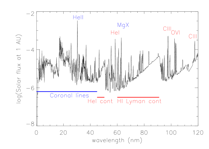
Figure 1: The Solar Irradiance Reference Spectrum (SIRS) obtained at solar minimum (March–April 2008). Flux units are Wm^-2nm^-1 at 1 AU. Important emission lines and continua are identified.

Figure 1 shows the composite irradiance spectrum at solar minimum (March–April 2008, Carrington Rotation 2068) when the solar 10.7 cm flux was at a very low value of $69\times 10^{-22}$ W m^-2 Hz^-1. At this time, an observing campaign with four instruments in space (Woods et al., 2009) measured the Solar Irradiance Reference Spectrum (SIRS) between 0.1 and 2400 nm, which was kindly provided by Martin Snow. The 0.1–6.0 nm spectrum was observed with the XUV (soft X-ray) Photometer System (XPS) of the Solar EUV Experiment (SEE) (Woods et al., 2005) on the Thermosphere, Ionosphere, Mesosphere, Energetics, and Dynamics (TIMED) spacecraft. The rocket prototype EUV Variability Experiment (EVE) (Chamberlin et al., 2009) monitored the 6.0–105 nm spectral interval, and the EUV Grating Spectrograph (EGS) on SEE obtained the 105–116 nm spectral interval. The 116–310 nm spectrum was measured by the Solar Radiation and Climate Experiment (SORCE) spectrometer on the Solar Stellar Irradiance Comparison Experiment (SOLTICE) satellite (McClintock et al., 2005).

Tom Woods has kindly provided a second set of solar irradiance data for times of solar minimum and maximum. These data were obtained with the SEE instrument on TIMED using the version 11 calibration. The solar minimum data are for day 105 in 2008, and the solar maximum data are for day 76 in 2002. We refer to this data set as the SEE data. Table 1 lists the SIRS and SEE fluxes in different wavelength bands.

Despite very careful contamination control and calibration before launch (e.g., Chamberlin et al., 2009; Hock et al., 2012), EUV spectrometers pointed at the Sun for long periods of time typically show sensitivity degradation due to contaminated optics and detector aging (BenMoussa et al., 2013). The 6.0–105 nm data in the SIRS data set should show minimal degradation as the spectrometer flew on a rocket and was calibrated before and after flight. The SEE data set, however, could include larger degradation, which is difficult to calibrate, as the solar minimum and maximum data were obtained six years apart with the same instrument in orbit.

2.2 Stellar 91.2–117.0 nm Spectra

With its LiF and SiC overcoated optics, the Far Ultraviolet Spectrograph Explorer (FUSE) satelite was able to observe nearby stars at wavelengths between the Lyman continuum bound-free edge at 91.2 nm and 117.0 nm. For a description of the FUSE satellite and observing program see Moos et al. (2000) and Sahnow et al. (2000). Redfield et al. (2002) described FUSE spectra of seven A7 V to M0 V stars, and Dupree et al. (2005) described FUSE spectra of eight F–M giants. The 91.2–117.0 nm spectrum is dominated by emission in Ly$\beta$ and higher Lyman lines (hereafter called the Lyman series) and emission lines of C II 103.6 nm, C III 97.7 nm, and O VI 103.2 and 103.8 nm. The Lyman lines are formed in the chromosphere at $\log T\approx 3.8$, C II lines near the base of the transition region ($\log T\approx 4.3$), and the C III and O VI lines in the transition region at $\log T\approx 4.8$ and 5.5, respectively. Much of the flux in the Lyman lines is absorbed or scattered by interstellar H I, and the lines are contaminated by terrestrial airglow emission (Feldman et al., 2001) that could not be removed accurately from the FUSE data. The weak continuum of F–G stars could not be measured by FUSE.

The quiet Sun spectrum described above likely provides a reliable census of the emission lines that dominate this portion of the spectrum for F–G stars. The brightest emission line in the 91.2–117.0 nm spectrum of the quiet Sun is the C III 97.70 nm line with flux of 0.101 erg cm^-2 s^-1 at 1 AU. The next brightest line is Ly$\beta$ with 0.0655 erg cm^-2 s^-1. The total flux in the Lyman series is only 0.114 in these units, whereas the sum of the fluxes in the C II, C III, and O VI lines is 0.178 in the same units. Since transition region lines are important contributors to the 91.2–117 nm flux of the quiet Sun, it is a sensible assumption, as confirmed by FUSE spectra, that the same transition region lines will also be important in this wavelength interval in F–M dwarfs stars. However, the relative strength of transition region lines may depend on stellar spectral type and activity. For example, the O VI lines are fainter than the C III line for the F and G stars Procyon and $\alpha$ Cen A, are comparable in brightness for the K dwarfs $\alpha$ Cen B and $\epsilon$ Eri, and are brighter than the C III line for the active M dwarf AU Mic (Redfield et al., 2002). There are also two coronal emission lines in this spectral range, Fe XVIII 97.486 nm and Fe XIX 111.806 nm, but these lines are very weak compared to the transition region lines (Redfield et al., 2003).

Redfield et al. (2002) provided a list of emission line fluxes, except for the Lyman series lines, for seven dwarf stars. Five of these stars have intrinsic Ly$\alpha$ fluxes measured by Wood et al. (2005): Procyon (F5 IV-V), $\alpha$ Cen A (G2 V), $\alpha$ Cen B (K0 V), $\epsilon$ Eri (K2 V), and AU Mic (M0 V). The sums of these emission line fluxes, except for the C III 117.5 nm blend that is observable by HST, are listed in Table 2.

2.3 Stellar 10–40 nm Spectra

The Extreme Ultraviolet Explorer (EUVE) obtained spectra of nearby stars in the 7–76 nm wavelength range with 0.05–0.2 nm spectral resolution. For a description of the EUVE science instruments, see Bowyer & Malina (1991) and Welsh et al. (1990). Craig et al. (1997) presented EUVE spectra for a variety of stars including several single and binary dwarf stars with F–M spectral types. Sanz-Forcada, et al. (2003) measured the emission line fluxes of many of these stars between 8 and 36 nm. We obtained calibrated EUVE spectra of 15 F–M dwarf stars with usable spectra between 10 and 40 nm from the Mikulski Archive for Space Telescopes (MAST) housed at the Space Telescope Science Institute (STScI). We downloaded only nighttime data for which scattered sunlight including geocoronal emission in the He II 30.4 nm line should be minimal. The stars selected (see Table 3) have good S/N, intrinsic Ly$\alpha$ fluxes (Wood et al., 2005; Linsky et al., 2013), and interstellar hydrogen column densities, log[N(HI)] (Wood et al., 2005). In a few cases, we have estimated intrinsic Ly$\alpha$ fluxes using correlations with other emission lines (e.g., Mg II, Ca II, and C IV) (Linsky et al., 2013). For a few stars we have also estimated interstellar hydrogen column densities using similar sight lines (Redfield & Linsky, 2008). Estimated parameters are listed in parentheses.

Table 3 summarizes the flux ratios in the 10–20, 20–30, and 30–40 nm bands that we obtained from the EUVE data. Listed in the Table are the EUVE data identifiers, EUVE observing times, spectral types, intrinsic Ly$\alpha$ fluxes, hydrogen column densities, and ratios of the EUVE flux in three wavelength bands to the Ly$\alpha$ flux before ($R$) and after correction for interstellar absorption ($R_{\rm ISM}$), using the interstellar absorption cross section formula of Morrison & McCammon (1983) computed for each wavelength. One EUVE spectrum of AU Mic (au_mic__9207141227N) is far brighter than the other two and contains a very large flare analyzed by Monsignori Fossi et al. (1996) and Cully et al. (1993). The other two observations of AU Mic show much weaker emission lines, and we assume represent the star’s quiescent emission. The EUVE spectrum of EV Lac also contains a large flare (Mullan et al., 2006). We have averaged two spectra of YZ CMi, two nonflare spectra of AU Mic, and 6 spectra of AD Leo that do not show evidence of large flares.

3 SOLAR MODELS

In this paper, we use the EUV fluxes computed with the new semiempirical solar models of Fontenla et al. (2013), which revise the chromosphere, transition region, and coronal structures of the earlier models of Fontenla et al. (2009) and Fontenla et al. (2011). The new models include updated collisional rates, ionization equilibria, and more levels and spectral lines from CHIANTI 7.1 (Landi et al., 2013). These are 1-dimensional non-LTE models of temperature vs. height structures selected to best fit the observed emitted intensity and spectral irradiance from the EUV to the infrared. The calculations in the updated models include 51 species of 21 elements at various stages of ionization and H^-. For the higher ionization stages, the level populations are computed using an ”effectively optically thin” approach, but optical thickness is considered for some lines-of-sight.

The updated set of nine models is defined by corresponding levels of magnetic heating as observed in chomospheric, transition-region, and coronal emissions (e.g., Ca II H and K lines, the 1600 Å continuum, and SOHO/EIT and SDO/AIA images). These models range from minimal activity (feature A represents quiet-Sun inter-network regions) to maximum activity (feature Q represents very hot plage). The solar feature designation (letter) and current photosphere-chromosphere-transition region (below 200,000 K) model index are, in order of increasing brightness, 1300 for A, 1301 for B, 1302 for D, 1303 for F, 1304 for H, 1305 for P, and 1308 for Q. The corresponding models for temperatures above 200,000 K including the corona are 1310–1318. and combination of the lower and higher temperature models are designated 13x0–13x8. In the earlier models, sunspot umbra and penumbra were included, but the updates were made only for the models listed above, which are the important ones for the EUV and FUV radiation. The solar spectral irradiance, the solar flux at 1 AU, is obtained from radiative transfer calculations of the intensity at 10 positions across the solar disk. The synthesized quiet-Sun computed spectrum matches the 116–168 nm irradiance at solar minimum activity measured by the SORCE/SOLSTICE instrument (Woods et al., 2009) and the 6–105 nm flux obtained by the EVE instrument (Chamberlin et al., 2009). Fontenla et al. (2013) conclude that the higher computed continuum in the 168-200 nm range compared to observations is due to a missing opacity source that is likely molecular. Computed fluxes of most important chromospheric and transition region emission lines are consistent with observations, although fine details of the lines are not perfectly matched by these very simplified models. Overall, the match to the observed EUV spectra is very good, as will be described later.

Since the Fontenla et al. (2013) models refer to the same star but with different levels of EUV and UV emission indicative of different levels of magnetic heating (often called “activity”), these models are very useful for studying correlations of EUV emission with many emission lines formed in the chromosphere and transition region as a function of activity for solar-like stars. Linsky et al. (2012) showed that the 115–150 nm continuum emission from Models 1001 through 1005 (Fontenla et al., 2011) corresponds to the observed continuum emission from low activity old solar-mass stars ($\alpha$ Cen A) to high activity young solar-mass stars (EK Dra and HII 314).

4 PREDICTING STELLAR FLUXES FROM CORRELATIONS WITH LY$\alpha$

4.1 The 91.2–117 nm Portion of the EUV Spectrum

We need to add the flux in the Lyman series lines beginning with Ly$\beta$ to the other emission lines for the five stars measured by Redfield et al. (2002). Lemaire et al. (2012) and previous authors that they cite noted that the Ly$\beta$/Ly$\alpha$ flux ratio increases with solar activity. This is likely due to the higher temperatures and thus higher collisional excitation rates in more active regions on the Sun. Flux in the other Lyman series lines should also increase faster than Ly$\alpha$ for the same reason. Figure 2 shows that the Lyman series/Ly$\alpha$ flux ratio increases from the least active area of the Sun (Fontenla et al., 2013) model 13x0 to the most active area (model 13x8). We fit these data with a power-law, log[f(Lyman series)/f(Ly$\alpha$)] = A + B log[f(Ly$\alpha$)], where A=–1.798 and B=0.351. Table 2 shows the sum of the emission line fluxes measured by Redfield et al. (2002), the estimated Lyman series flux using the above relation, the total flux in the 91.2–117.0 nm band, and the ratio of this flux to f(Ly$\alpha$).

Figure 3 shows the ratio of the total 91.2–117.0 nm flux to the Ly$\alpha$ flux (the EUV flux ratio) for the solar models and the solar and stellar data. The asterix symbols and solid line connecting them in Figure 3 are the EUV flux ratios obtained from the Fontenla et al. (2013) semiempirical models 1300 to 1308. The Sun symbol is for the observed quiet Sun ratio in the SIRS data set, and the “m” and “M” symbols refer to the solar minimum and maximum data for the SEE data set. We note that the solar data lie only about 0.10 dex below the quiet and moderately active solar models 1300–1302.

Since we are comparing EUV flux ratios among stars with different radii, we plot the EUV flux ratios in this and subsequent figures, vs. the stellar Ly$\alpha$ flux at 1 AU multiplied by the scale factor $(R_{Sun}/R_{star})^{2}$. This scale factor enables us to compare the EUV flux ratios to the Ly$\alpha$ flux per unit area of the stellar surface, which is a physical measure of the chromospheric heating rate. There is no need to scale either the EUV flux or Ly$\alpha$ flux when computing the EUV flux ratios as both quantities are proportional to the stellar radius and the ratio is thus independent of stellar radius.

The flux in the Lyman series lines beginning with Ly$\beta$ is only about 20% of the total 91.2–117.0 nm flux for the quiet Sun models, but it increases to 30% for the active Sun models. This suggests that similar ratios likely apply to stars with similar activity levels as measured by the Ly$\alpha$ flux. We therefore add the estimated Lyman series fluxes to the observed 91.2–117.0 nm line fluxes for the five stars observed by FUSE and divide the sums by the reconstructed Ly$\alpha$ fluxes (Linsky et al., 2013). The error bars for each star are estimates that include the estimated Lyman series fluxes, assuming errors in both dimensions of $\pm 15$%.

The least-squares fit power law to flux ratio vs. scaled Ly$\alpha$ flux for the five stars and the Sun is log[f(91.2–117.0 nm)/f(Ly$\alpha$)] = C + D log[f(Ly$\alpha$)], where C=$-1.189\pm 0.202$ and D=$+0.110\pm 0.152$. Since the uncertainty in the linear coefficient is larger than its value, we instead fit the data with a constant value log[f(91.2–117.0 nm)/f(Ly$\alpha$)] = -1.025. The mean dispersion of the solar and stellar data about this relation is only 29.5% and the rms dispersion is 35.0%. Since this fit (dash-dot line) in Figure 3 provides an excellent fit to the solar and F5 IV-V to M0 V stellar data, we argue that it can be used to predict the 91.2–117.0 nm flux from a wide range of late-type dwarf stars, provided one has measurements of the Ly$\alpha$ flux or another spectral line that is correlated with the Ly$\alpha$ flux. Note that the empirical fit is an excellent match to the solar data and to $\alpha$ Cen A, which is a close match to the Sun. The solar models (solid line in Figure 3) lie only 0.1–0.2 dex above the empirical fit to the solar and stellar data. While the contribution of the 91.2–117.0 nm band to the total flux incident on an exoplanet is relatively small compared to the flux in Ly$\alpha$, it will be important for the photodissociation of molecules that have peak cross-sections in this wavelength range (e.g., CO and H₂).

4.2 The Hydrogen Lyman Continuum 60–91.2 nm

The solar spectrum (Figure 1) shows that the hydrogen Lyman continuum emission extends from the 91.2 nm edge down to nearly 60 nm. The brightest emission lines superimposed on the Lyman continuum are lines of O III (near 84 and 72 nm), O IV (near 79 nm), Ne IV and Ne VIII (76–78 nm), and a mixture of other transition region lines at shorter wavelengths. We now consider how to isolate the Lyman continuum component of the EUV spectrum and then compare its flux to observable emission features.

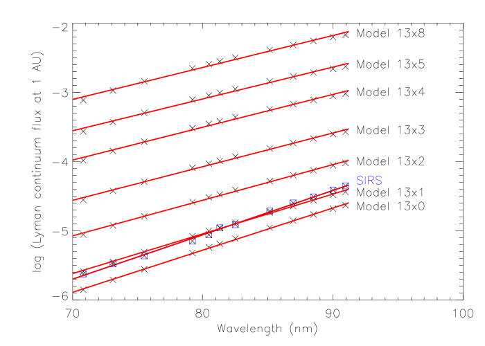
Figure 4: Plots of the Lyman continuum flux (Wm^-2nm^-1) at a distance of 1 AU for the quiet Sun SIRS data set and for the semiempirical solar irradiance models of Fontenla et al. (2013). X-symbols are fluxes for spectral regions with no apparent emission lines. Box symbols are for the SIRS data. Solid red lines are least-squares fits to the data.

Figure 4 shows the SIRS Lyman continuum flux measured at 12 wavelengths where there is no obvious blending with weak emission lines. The solid line is a least-squares linear fit in this semilog plot with $f(\lambda)=5.85\times 10^{-11}e^{-0.149\lambda}$ erg cm^-2 s^-1, where $\lambda$ is in nm. The fit is very good with an rms deviation of 3.9%. Parenti, Lemaire, & Vial (2005) have previously shown that an exponential provides a very good fit to the Lyman continuum slope in the SOHO/SUMER radiance data. The integrated flux in the Lyman continuum between 60 and 91.2 nm is 0.307 erg cm^-2 s^-1 at 1 AU or 5.16% that of the Ly$\alpha$ flux in the same data set. By comparison, the total flux in the Lyman line series is only 0.114 erg cm^-2 s^-1 or 1.92% of the Ly$\alpha$ flux. Thus the Lyman continuum flux is 2.7 times brighter than the Lyman series lines (see Table 4).

We also plot in Figure 4 the Lyman continuum flux for the Fontenla et al. (2013) models at the same wavelengths. These fluxes are also well fit by straight lines in these semilog plots. Note that the observed quiet Sun (SIRS) Lyman continuum fluxes are similar to those of Model 13x1 and that the slopes of the model data steepen with decreasing solar activity. Because of the short wavelengths in the Lyman continuum compared to chromospheric temperatures, the slopes of the continuum flux vs. wavelength are well fit by Wien’s approximation to the Planck function, and the color temperatures obtained from the slopes are a good measure of the temperature where the optically thick continuum is formed. We include in Table 4 the total Lyman continuum fluxes, ratios to the Ly$\alpha$ flux, and the color temperatures. The Lyman continuum flux, ratio to Ly$\alpha$, and color temperature of the SIRS data set are all similar to Model 1301.

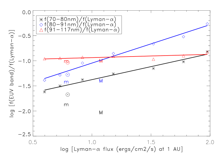
Figure 5: Plots of the ratios of the fluxes in the 70–80 nm, 80–91.2 nm, and 91.2–117 nm wavelength bands divided by the Ly$\alpha$ flux. The symbols are total fluxes in each wavelength band for Fontenla et al. (2013) models 13x0 to 13x8 (left to right). The solid lines are least-squares fits to each data set. The Sun symbols are for the SIRS quiet Sun fluxes in these wavelength bands, and the “m” and “M” symbols are the solar minimum and maximum data obtained with the SEE experiment on the TIMED spacecraft for the wavelength bands. The 80–91.2 nm passband is mainly Lyman continuum flux, whereas the 70–80 nm passband contains strong transition-region lines of O III, O IV, and N IV that are likely overestimated in the models.

Figure 5 shows a comparison of the ratios of fluxes in the 70–80 nm, 80–91.2 nm, and 91.2–117 nm wavelength bands to the Ly$\alpha$ flux. The solid lines are least-squares fits to the EUV/Ly$\alpha$ flux ratios for the Fontenla et al. (2013) models. The Lyman continuum is the largest contributor to the 80–91.2 nm wavelength band, but bright emission lines of O III, O IV, and N IV dominate the 70–80 nm passband. The SIRS and SEE solar data points for the 91.2–117 nm passband are in excellent agreement with the model predictions. For the 80–91 nm and 70–80 nm wavelength bands, the SIRS data agree with the models better than the SEE data.

4.3 The 10–60 nm Portion of the EUV Spectrum

The spectrum below 60 nm includes a number of features formed in the chromosphere, including the He I continuum visible between 45 and 50.4 nm and emission lines of He I (58.4 and 53.7 nm) and He II (30.4 and 25.6 nm). He II 30.4 nm is the brightest emission line in the 10–91.2 nm region. This line is formed primarily by collisional excitation in the chromosphere, but a portion of the emission is recombination following photoionization of He⁺ by coronal radiation (Avrett et al., 1976). There are also a number of transition region lines of O II, O III, O IV, and N III located in this spectral region. Beginning with the Mg X (61.0–62.5 nm) and Si XII (49.9–52.1 nm) multiplets, coronal emission lines increasingly dominate the spectrum at shorter wavelengths. Thus the 10–60 nm portion of the EUV spectrum of the quiet Sun is a combination of emission from the chromosphere, transition region, and corona.

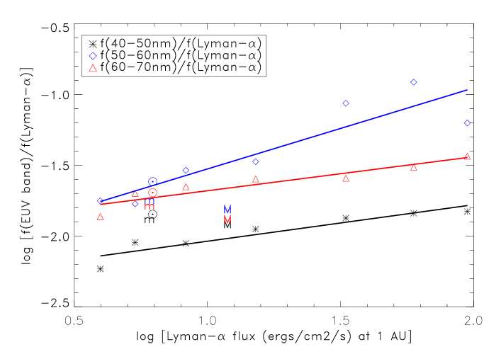
Figure 6: Same as Figure 5 except for the 40–50 nm, 50–60 nm, and 60–70 nm wavelength bands.

Figure 6 compares the EUV/Ly$\alpha$ flux ratios with the Fontenla et al. (2013) models and the SIRS and SEE solar reference data. The agreement of the SIRS and quiet Sun SEE data with the models is very good, but the active Sun SEE data are low compared to the models for the 50–60 nm and 60–70 nm wavelength bands. In the absence of any stellar data for comparison with the solar ratios or models, we suggest using least-squares fits to the models with the parameters listed in Table 5.

At wavelengths shorter than about 40 nm, modest interstellar absorption to the nearest stars permits detection of EUV radiation, thereby providing empirical tests of the accuracy with which the solar data and models can provide estimates of the EUV flux ratios for different spectral type stars. We compare in Figure 7 the solar 10–20 nm flux ratios to EUVE flux ratios (corrected for interstellar absorption) $R_{\rm ISM}$ versus scaled Ly$\alpha$ fluxes for 15 stars with spectral types between F5 IV-V (Procyon) and M5.5 V (Proxima Centauri). The least-squares fit to the data for the F5–K7 stars is log[f(10–20 nm)/f(Ly$\alpha$)] = $-1.357\pm 0.127$ + $0.344\pm 0.094$ log[f(Ly$\alpha$)]. The mean deviation about this fit line is 20.5% and the rms deviation is 29.0%. There is no apparent trend with spectral type. Excluding the EV Lac and AU Mic flare data (see later in this section), the remaining five M stars have nearly the same EUV flux ratios. Since the linear coefficient in the least-squares fit to these data is smaller than its uncertainty, we fit the data with a constant value, log[f(10–20 nm)/f(Ly$\alpha$)] = –0.491. The M star flux ratios have a small mean deviation of 12.6% and a small rms deviation of 15.1%. Also plotted in Figure 7 are flux ratios for the Fontenla et al. (2013) models. The flux ratios of $\alpha$ Cen A+B and Procyon are very close to the quiet Sun models and data, and the flux ratios for the other G- and K-type stars are also consistent with the solar model ratios. Our recommend fitting relations are summarized in Table 5.

Figure 8 is a similar comparison of solar and stellar data and solar model flux ratios for the 20–30 nm wavelength region. The least-squares fit to the data for the F5–K7 stars is log[f(10–20 nm)/f(Ly$\alpha$)] = $-1.300\pm 0.224$ + $0.309\pm 0.164$ log[f(Ly$\alpha$)] with a mean deviation of 47.6% and an rms deviation of 56.6%. Again excluding the EV Lac and AU Mic flare data, the five M stars can be fit by log[f(20–30 nm)/f(Ly$\alpha$)] = –0.548. The mean deviation about this fit is 24.3% and the rms deviation is 26.9%. The solar model ratios are consistent with the $\alpha$ Cen A+B and the other F-, G-, and K-star data.

Finally, Figure 9 shows a similar plot for the 30–40 nm data. Since the interstellar absorption corrections exceed a factor of 3 for this bandpass when log [N(H I)] $>18.2$, the flux ratios for AU Mic and AD Leo depend critically on the uncertainties in the N(H I) parameter. The models fit the solar data well, but have a slightly different slope than the F5 V–K7 V stars. Since the linear coefficient in the least-squares fit to the F5–K7 stellar flux ratios is consistent with zero, we fit these data with log[f(30–40 nm)/f(Ly$\alpha$)] = –0.882, with a mean deviation of 37.1% and an rms deviation of 41.0%. The M star flux ratios, except for the two flaring stars, can be fit with log[f(30–40 nm)/f(Ly$\alpha$)] = –0.602 with a mean deviation of 18.9% and an rms deviation of 20.5%. Table 5 summarizes these fits and the dispersions of the stellar data points about these fits.

Since we do not have Ly$\alpha$ fluxes for EV Lac and AU Mic during their flares, we consider two different ways of representing their flare flux ratios. In Figures 7–9, we plot the ratios of the observed EUV flare fluxes divided by the reconstructed quiesent Ly$\alpha$ fluxes vs. the scaled quiescent Ly$\alpha$ fluxes. This almost certainly overestimates the flux ratios and places the data points at unrealistically low scaled Ly$\alpha$ flux levels. The dashed lines extending downwards and to the right in the figures show the location of the ratios with increasing Ly$\alpha$ flux. The correct ratios should lie along these dashed lines. We estimate the most likely values of the Ly$\alpha$ flux during the flares by noting the factors by which the EUV fluxes during the flare of AU Mic exceed the quiescent values and using the formulae in Table 5. The symbols at the lower right end of the dashed lines in the figures indicate the most likely values for the flare ratios and scaled Ly$\alpha$ fluxes for the two stars. These flare ratios are close to the mean nonflare ratios for M dwarf stars, indicating that the fits obtained using the quiescent M star data should be useful for estimating EUV fluxes of M dwarfs over a wide range of activity, provided the Ly$\alpha$ flux is appropriate for the given level of activity.

4.4 Errors in the Flux Ratio Estimates

There are three sources of error in our technique: errors in the EUV fluxes, errors in the reconstructed Ly$\alpha$ fluxes, and errors associated with stellar variability since the EUV and Ly$\alpha$ fluxes were not obtained at the same time. The mean and rms dispersions about the fit lines reflect all three sources of error. The uncertainties in the Ly$\alpha$ reconstructions are probably in the range 10–30%, depending on the quality of the observations and the complexity of the interstellar medium velocity structure. The dispersions for the F5–K5 stars about the fits lie in the range 20–37%. This is consistent with errors in the EUV fluxes and errors associated with stellar variability each being in the range of 10–20%. The dispersions for the M stars are smaller, 13–24%. Although this was unexpected, it may result from the exclusion of obvious flaring events during the measurements of the Ly$\alpha$ and EUV fluxes. Also the M stars are located closer to the Sun than the F5–K5 stars, in which case the velocity structure of the ISM should be simpler and the Lyman$\alpha$ reconstructions more reliable. Expansion of the M star data set would be helpful in understanding the relative contributions of the three components to the dispersions.

5 DISCUSSION

Sanz-Forcada et al. (2011) (hereafter SF2011) developed a technique for predicting EUV fluxes based on an emission measure analysis of observed stellar X-ray spectra. This method predicts the emission line spectrum between 0.1 and 91.2 nm but may not accurately include the Lyman continuum, important between 70 and 91.2 nm, or the He I and He II continuua below 50.4 nm and 22.8 nm. In Table 6, we compare predicted EUV flux ratios for the five stars in SF2011 Table 4 for which Linsky et al. (2013) list Ly$\alpha$ fluxes.

We checked MAST to find that only one star, $\epsilon$ Eri, listed in Table 4 of SF2011 was observed spectroscopically by EUVE. In the 10–20 nm band, the flux ratio predicted using our formula (see Table 6) and SF2011 are both consistent with the EUVE spectrum of $\epsilon$ Eri corrected for interstellar absorption, $R_{\rm ISM}$. In the 20–30 nm band, our formula predicts a flux ratio 0.22 dex below the EUVE data and the SF2011 prediction is 0.09 dex larger than the EUVE data. In the 30–40 nm band, the SF2011 prediction is 0.07 dex larger than observed by EUVE, and our formulae predicts a flux ratio 0.14 dex smaller. In the 70–91.2 nm band, where the Lyman continuum is an important contributor to the emission, the inclusion of the Lyman continuum flux would likely place the SF2011 ratio about 0.3 dex above our model prediction for $\epsilon$ Eri.

The four other stars listed in Table 6 without EUVE spectroscopic data show no clear pattern in the predicted flux ratios based on our formulae and SF2011. For HD 209458 (G0 V), the upper limits predicted by SF2011 all lie below, and at some wavelengths far below, the flux ratios predicted by our formulae. This highlights the problem of computing emission measure distributions based on very weak or upper limits to the X-ray fluxes. For HD 189733 (K1 V), the flux ratios predicted by SF2011 are systematically high compared to our formulae, and for GJ 436 (M3 V) they are systematically low compared to our formulae. For GJ 876 (M5.0 V) the SF2011 flux ratios are very low compared to our formulae in the 10–20 and 20–30 nm bands, but comparable in the longer wavelength bands.

Finally, we compare in Table 6 the 91.2–117 nm flux ratios predicted by our formulae with the fluxes obtained using the emission measure analysis technique listed in the X-exoplanets website described in SF2011 divided by the reconstructed Ly$\alpha$ fluxes (Linsky et al., 2013). The flux ratios computed from the predicted fluxes in the X-exoplanets website are 0.6–2.5 dex below those predicted by our formulae. The excellent $\epsilon$ Eri FUSE data provide a clear test of the two prediction methods. The f(91.2–117 nm)/f(Ly$\alpha$) ratio obtained from the FUSE emission line fluxes (Redfield et al., 2002) and estimated Lyman series flux is 0.2 dex below that predicted by our method but 0.9 dex above that obtained from the data in the X-exoplanets website. The missing flux in the X-exoplanet website predictions likely indicates the inadequate treatment of emission lines formed at temperatures below $2\times 10^{5}$ K.

6 CONCLUSIONS

EUV fluxes from host stars control the photochemistry, heating, and mass loss from the outer atmospheres of exoplanets, especially for those exoplanets located close to their host stars. The objective of this study is to develop a useful technique for predicting the EUV fluxes of F5–M5 dwarf stars, since there are only a few measurements of stellar EUV fluxes and interstellar absorption prevents measurements between 40 and 91.2 nm for all nearby dwarfs stars except for the Sun. Our technique employs ratios of EUV fluxes in wavelength bands to the Ly$\alpha$ flux, because models of the solar chromosphere, transition region, and corona show that the EUV flux scales with the Ly$\alpha$ flux. Moreover, models of solar regions with different amounts of magnetic heating show temperature structures with similar shapes but displaced deeper into the atmosphere (and thus higher densities) with increasing magnetic heating. These empirical and theoretical arguments gives us confidence that the ratios of the EUV flux in various wavelength bands to the Ly$\alpha$ flux should vary smoothly with stellar activity at least for stars that do not differ too greatly from the Sun in spectral type. Models of stellar chromospheres and transition regions comparable in detail with the solar models of Fontenla et al. (2013) are needed to confirm the range of stars for which our technique is useful. Until such models are available, observations of the few stars in the 91.2–117.0 nm range by the FUSE satellite and in the 10–40 nm range by the EUVE satellite show that our ratio technique is useful for F5–M5 dwarfs.

Table 5 summarizes our recommended formulae for predicting the log [f($\Delta\lambda$)/f(Ly$\alpha$)] ratios in nine wavelength bands. For the 10–20 nm, 20–30 nm, and 30–40 nm wavelength bands, we recommend using the formulae based on the stellar fluxes observed by EUVE. Our formulae predict flux ratios similar to the observations and to the emission measure analysis predictions of SF2011, as indicated by comparison with the EUVE data for $\epsilon$ Eri. For the 40–91.2 nm wavelength range, where there are no reliable stellar observations to compare with the solar fluxes or models, we suggest using the formulae based on the Fontenla et al. (2013) solar models to predict flux ratios for F7–K7 dwarf stars. For M stars, we suggest adding 0.2 dex to the solar ratios, the mean displacement of the M stars from the warmer stars in the 20–30 and 30–40 nm bands. In the 91.2–117 nm band, the agreement between the FUSE data and our model predictions shown in Figure 3 suggests that the ratios for M stars may be the same as for the warmer stars. Fits to the flux ratios based on the FUSE data and our formulae are in good agreement. On the other hand, the predictions of the emission measure analysis models in the X-Exoplanets website are far below our models and the FUSE observations of $\epsilon$ Eri. Figures 7–9 and Table 5 show that for the F5–K5 stars the mean deviations from the fit lines lie in the range 20–48%, and for the nonflaring M stars the mean deviations lie in the range 12–24%. Thus our formulae should be useful in predicting the EUV flux ratios for F5–M5 dwarf stars. We note that the flux ratios based on the Fontenla et al. (2013) solar models closely match the solar data, as expected, but they also come remarkably close to matching the stellar flux ratios.

Figure 2: Ratio of the Lyman series flux from Ly$\beta$ to 91.2 nm divided by the Ly$\alpha$ flux for the Fontenla et al. (2013) semiempirical models 13x0 to 13x8 (asterix symbols from left to right). The solid line is a least-squares fit to the data points. The SIRS flux ratio is represented by the solar symbol.

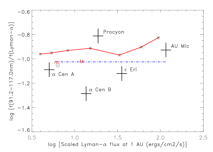
Figure 3: Ratios of the total flux between 91.2 and 117.0 nm divided by the Ly$\alpha$ flux at 1 AU scaled by the ratio of stellar radii, $(R_{Sun}/R_{star})^{2}$. The solid-line-connected asteriskes (red line) are the total flux in this passband for the Fontenla et al. (2013) semi-empirical models 13x0 to 13x8 (from left to right). Flux ratios for five stars based on FUSE spectra and reconstructed Lyman series fluxes are shown as $\pm 15$% error bar symbols. The Sun symbol is the ratio for the SIRS quiet Sun data set. The dash-dot (blue) line is the least-squares fit to the stellar and SIRS data. The “m” and “M” symbols are the solar minimum and maximum data obtained with the SEE instrument on the TIMED spacecraft (Woods et al., 2005).

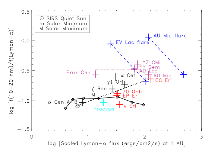
Figure 7: Ratios of the intrinsic flux between 10 and 20 nm (corrected for interstellar absorption) divided by the reconstructed Ly$\alpha$ flux vs. the reconstructed Ly$\alpha$ flux at 1 AU scaled by the ratio of stellar radii, $(R_{Sun}/R_{star})^{2}$. The solid line-connected diamonds are the total flux ratios in this passband for the Fontenla et al. (2013) semiempirical models 13x0 to 13x8 (from left to right). Flux ratios for one F star (cyan), four G stars (black), four K stars (red), and five M stars (plum) based on EUVE spectra are shown as $\pm 15$ error bar symbols. The dash-dot (black) line is the least-squares fit to the solar and F, G, and K star ratios. The plum dash-dot line is the mean of the M star ratios excluding the EV Lac flare and AU Mic flare data. Flux ratios for EV Lac and AU Mic during flares (blue) are plotted two ways. The upper left symbols are ratios of EUV flare fluxes to quiescent Ly$\alpha$ fluxes. Dashed lines extending to the lower right indicate the ratios for increasing Ly$\alpha$ flux. The symbols at the lower end of the dashed lines are ratios obtained using the most likely values of the Ly$\alpha$ fluxes during flares (see text). The “m” and “M” symbols are the solar minimum and maximum data obtained with the SEE instrument on the TIMED spacecraft (Woods et al., 2005). The Sun symbol is the ratio for the SIRS quiet Sun data set.

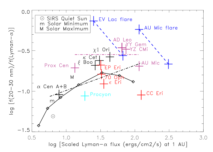
Figure 8: Same as Figure 7 except for the 20–30 nm wavelength interval.

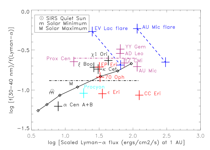
Figure 9: Same as Figure 7 except for the 30–40 nm wavelength interval.

Table 1: Solar EUV Fluxes (erg cm^-2 s${-1}$) in Wavelength Bands

Wavelength	SIRS (Solar Minimum)		SEE (Solar Minimum)		Solar Maximum
Band (nm)	f(EUV)	f(EUV)/f(Ly$\alpha$)	f(EUV)	f(EUV)/f(Ly$\alpha$)	f(EUV)	f(EUV)/f(Ly$\alpha$)
Ly$\alpha$	5.95		5.78		11.5
10–20nm	0.451	0.0758	0.440	0.0761	1.35	0.118
20–30nm	0.276	0.0465	0.422	0.0730	1.64	0.143
30–40nm	0.548	0.0921	0.514	0.0889	1.33	0.115
40–50nm	0.0788	0.0132	0.0718	0.0124	0.316	0.0144
50–60nm	0.134	0.0225	0.0977	0.0169	0.166	0.0145
60–70nm	0.112	0.0188	0.0890	0.0154	0.141	0.0123
70–80nm	0.115	0.0193	0.0721	0.0125	0.0995	0.00865
80–91.2nm	0.287	0.0483	0.204	0.0354	0.426	0.0370
91.2–117nm	0.502	0.0844	0.527	0.0911	1.060	0.0922
117–130nm-Ly$\alpha$			0.538	0.0930	0.779	0.0677
130–140nm			0.543	0.0939	0.811	0.0705
140–150nm			0.558	0.0965	0.689	0.0599
150–160nm			1.367	0.237	1.634	0.142
160–170nm			3.174	0.549	3.631	0.316
170–180nm			9.831	1.701	11.23	0.977

Table 2: Stellar Fluxes (ergs cm^-2 s^-1) at 1 AU in Different Wavelength Bands

Parameter	Procyon	SIRS	$\alpha$ Cen A	$\alpha$ Cen B	$\epsilon$ Eri	AU Mic
Spectral Type	F5 IV-V	G2 V	G2 V	K0 V	K1 V	M0 V
d(pc)	3.50		1.325	1.255	3.216	9.91
Age(Gyr)	1.85	4.566	$4.4\pm 0.5$	$4.4\pm 0.5$	0.43	$0.020\pm 0.010$
f(Ly$\alpha$)	77.1	5.95	7.54	10.1	21.5	43.0
f(FUSE data without Lyman lines)	6.46		0.374	0.168	0.650	2.61
f(Lyman series)	5.41	0.242	0.239	0.354	0.976	2.47
f(91.2–117.0 nm)	11.87	0.507	0.613	0.522	1.626	5.08
f(91.2–117.0 nm)/f(Ly$\alpha$)	0.154	0.0852	0.0813	0.0517	0.0756	0.118

Table 3: Ratios of EUVE Fluxes in Wavelength Bands Divided by the Intrinsic Ly$\alpha$ Fluxes

Star	$R_{\star}/R_{\odot}$	EUVE ID	f(Ly$\alpha$)	log[N(HI)]	10–20 nm		20–30 nm		30–40 nm
		(ks)			log$R$	log$R_{\rm ISM}$	log$R$	log$R_{\rm ISM}$	log$R$	log$R_{\rm ISM}$
Procyon (F5 IV-V)	2.03	procyon__9403122334N	77.1	18.06	–1.100	–1.032	–1.223	–1.058	–1.376	–1.040
$\chi^{1}$ Ori (G0 V)	0.98	chi1_ori__9301261159N	41.6	17.93	–0.780	–0.736	–0.713	–0.577	–0.890	–0.631
$\alpha$ Cen (G2 V+K0 V)	1.50	alpha_cen_9703100800N	17.64	17.61	–1.052	–1.028	–1.100	–1.042	–1.316	–1.203
$\kappa$ Cet (G5 V)	0.99	kappa_cet__9510061036N	30.0	17.89	–0.645	–0.608	–0.738	–0.622	–0.985	–0.739
$\xi$ Boo (G8 V+K4 V)	1.16	xi_boo__9704200202N	35.3	17.92	–0.849	–0.806	–0.807	–0.681	–0.958	–0.715
70 Oph (K0 V+K4 V)	1.13	gj_702__9307021144N	23.6	18.06	–0.942	–0.878	–0.960	–0.790	–1.190	–0.839
$\epsilon$ Eri (K1 V)	0.78	eps_eri__9509051851N	21.5	17.88	–1.104	–1.063	–1.024	–0.909	–1.270	–1.046
EP Eri (K2 V)	0.93	gj_117__9412020500N	27.6	18.05	–0.976	–0.916	–0.853	–0.678	–1.051	–0.713
CC Eri (K7 V)	0.66	cc_eri__9509130049N	(54)	(18.1)	–0.690	–0.640	–1.211	–1.046	–1.433	–1.064
AU Mic flare (M0 V)	0.61	au_mic__9207141227N	43.0	18.36	–0.034	+0.050	–0.564	–0.238	–0.894	–0.233
AU Mic (M0 V)	0.61	Mean	43.0	18.36	–0.663	–0.571	–1.068	–0.691	–1.362	–0.708
YY Gem (dM1e+dM1e)	0.88	yy_gem__9502201531N_1	(50.0)	(18.0)	–0.511	–0.471	–0.614	–0.463	–0.784	–0.489
EV Lac flare (M3.5 V)	0.35	ev_lac__9309091718N	3.07	17.97	–0.103	–0.061	–0.272	–0.134	–0.556	–0.269
AD Leo (M3.5 V)	0.38	Mean	9.33	18.47	–0.602	–0.481	–0.949	–0.465	–1.408	–0.543
YZ CMi (M4.5 V)	0.30	Mean	6.7	(17.8)	–0.421	–0.395	–0.584	–0.482	–0.848	–0.662
Prox Cen (M5.5 V)	0.15	proxima_cen__9305211911N	0.301	17.61	–0.580	–0.560	–0.775	–0.712	–0.771	–0.646

Table 4: Lyman line and Lyman continuum fluxes (erg cm^-2 s^-1) at 1 AU

Line	$\lambda$(nm)	SIRS	f(1300)	f(1301)	f(1302)	f(1303)	f(1304)	f(1305)	f(1308)
Ly$\beta$	102.57	0.0655	0.0422	0.0599	0.128	0.296	0.670	1.302	2.094
Ly$\gamma$	97.25	0.0155	0.0191	0.0267	0.0584	0.135	0.301	0.610	1.20
Ly$\delta$	94.97	0.0081	0.0119	0.0165	0.0369	0.0863	0.206	0.420	0.844
Ly$\epsilon$	93.78	0.00487	0.00765	0.0109	0.0244	0.0563	0.137	0.279	0.546
Ly7	93.08	0.00323	0.00496	0.00692	0.0160	0.0376	0.0988	0.208	0.416
Ly8	92.62	0.00186	0.00302	0.00426	0.0102	0.0251	0.0709	0.157	0.327
Ly9	92.31	0.0010	0.0019	0.0025	0.0067	0.0175	0.0556	0.128	0.279
Ly10	92.10		0.000738	0.000781	0.00320	0.0101	0.0404	0.0978	0.232
Ly11+rest	91.94		0.00555	0.00849	0.0238	0.0686	0.226	0.583	1.288
Sum		0.114	0.0969	0.137	0.308	0.732	1.80	3.78	7.22
Ly$\alpha$		5.95	3.96	5.35	8.30	15.17	33.11	59.52	94.68
Sum/Ly$\alpha$		0.0192	0.0245	0.0256	0.0371	0.0483	0.0545	0.0636	0.0763
Ly$\beta$/Ly$\alpha$		0.0110	0.0107	0.0112	0.0155	0.0195	0.0202	0.0219	0.0221
Ly$\alpha$/Ly$\beta$		90.84	93.86	89.33	64.64	51.22	49.45	45.70	45.22
f(91.2–117.0nm)		0.507	0.433	0.598	0.973	1.85	3.55	7.43	14.14
f(91.2–117.0)/f(Ly$\alpha$)		0.0852	0.109	0.112	0.117	0.122	0.107	0.125	0.149
Lycont		0.307	0.178	0.296	0.858	2.56	9.42	23.9	68.2
Lycont/Ly$\alpha$		0.0516	0.0449	0.553	0.103	0.169	0.285	0.402	0.720
Ly$\alpha$/Lycont		19.4	22.2	18.1	9.67	5.93	3.51	2.49	1.39
T(color) (K)		12,210	12,640	13,230	14,360	14,930	15,160	15,480	15,390

Table 5: Formulae for Estimating EUV Fluxes (erg cm^-2 s^-1) in Wavelength Bands

Wavelength	log[f($\Delta\lambda$/f(Ly$\alpha$)]
Band (nm)	F5–K7 V stars	M V stars	F5–M5 V stars
10–20nm (stars)	–1.357+0.344 log[f(Ly$\alpha$)]	–0.491
20–30nm (stars)	–1.300+0.309 log[f(Ly$\alpha$)]	–0.548
30–40nm (stars)	–0.882	–0.602
40–50nm (models)			-2.294+0.258 log[f(Ly$\alpha$)]
50–60nm (models)			-2.098+0.572 log[f(Ly$\alpha$)]
60–70nm (models)			-1.920+0.240 log[f(Ly$\alpha$)]
70–80nm (models)			-1.894+0.518 log[f(Ly$\alpha$)]
80–91.2nm (models)			-1.811+0.764 log[f(Ly$\alpha$)]
91.2–117nm (models)			-1.004+0.065 log[f(Ly$\alpha$)]
Lyman series (models)			-1.798+0.351 log[f(Ly$\alpha$)]
91.2–117nm (stars)			–1.025
10–20nm mean deviation	20.5%	12.6%
10–20nm rms deviation	29.0%	15.1%
20–30nm mean deviation	47.6%	24.3%
20–30nm rms deviation	56.6%	26.9%
30–40nm mean deviation	37.1%	18.9%
30–40nm rms deviation	41.0%	20.5%
91.2–117nm mean deviation			29.5%
91.2–117nm rms deviation			35.0%

Table 6: Comparison of EUV Flux Ratios log [f($\Delta\lambda$)/f(Ly-$\alpha$)]

Wavelengths	HD 209458	$\epsilon$ Eri	HD 189733	GJ 436	GJ 876
Data Set	G0 V	K1 V	K1 V	M3 V	M5.0 V
$\Delta\lambda$=10–20 nm
Model	–1.046	–1.025	–1.065	–0.583	–0.560
Sanz-Forcada	$<-2.625$	–1.092	–0.621	–2.385	–1.621
EUVE		–1.063
$\Delta\lambda$=20–30 nm
Model	–1.127	–1.126	–1.127	–0.909	–0.945
Sanz-Forcada	$<-1.945$	–0.822	–0.661	–1.985	–1.411
EUVE		–0.909
$\Delta\lambda$=30–40 nm
Model	–1.153	–1.186	–1.124	–1.003	–1.029
Sanz-Forcada	$<-1.575$	–0.972	–0.681	–1.435	–1.051
EUVE		–1.046
$\Delta\lambda$=40–70 nm
Model	–1.374	–1.374	–1.374	–1.074	–1.074
Sanz-Forcada	$<-1.481$	–1.195	–0.896	–1.306	–0.988
$\Delta\lambda$=70–91.2 nm
Model	–1.237	–1.237	–1.237	–0.942	–0.942
Sanz-Forcada	$<-1.295$	–1.290	–0.921	–1.165	–0.861
$\Delta\lambda$=10–91.2 nm
Model	–0.475	–0.522	–0.474	–0.166	–0.167
Sanz-Forcada	$<-0.905$	–0.342	–0.041	–0.775	–0.411
$\Delta\lambda$=91.2–117 nm
Model	–0.926	–0.917	–0.934	–0.991	–1.029
X-exoplanets	–2.482	–2.006	–1.688	–1.906	–1.619
FUSE+Ly series		–1.122

References

- Allegre et al. (1995) Allegre, C. J., Manhes, G., & Gopel, C. 1995, Geochim. Cosmochim. Acta, 59, 1445
- Avrett et al. (1976) Avrett, E. H., Vernazza, J. E., & Linsky, J. L. 1976, ApJ, 207, L199
- Ayres (1997) Ayres, T. R. 1997, J. Geophys. Res., 102(E1), 1641
- Ayres (2010) Ayres, T. R. 2010, ApJS, 187, 149
- Barnes (2007) Barnes, S. A. 2007, ApJ, 669, 1167
- Bisikalo (2013) Bisikalo, D., Kaygorodov, P., Shematovich, V., Lammer, H., & Fossati, L. 2013, ApJ, 764, 19
- BenMoussa et al. (2013) BenMoussa, A., Gissot, S., Schühle, U., et al. 2013, Solar Phys, in press
- Bowyer & Malina (1991) Bowyer, S. & Malina, R. F. 1991, in Extreme Ultraviolet Astronomy, ed. R. F. Malina & S. Bowyer (New York: Pergamon), 333
- Chamberlin et al. (2009) Chamberlin, P. C., Woods, T. N., Crotser, D. A., Eparvier, F. G., Hock, R. A., & Woodraska, D. M. 2009, J. Geophys. Res., 36, 5102
- Claire et al. (2012) Claire, M. W., Sheets, J., Cohen, M., Ribas, I., Meadows, V. S., & Catling, D. C. 2012, ApJ, 757, 95
- Craig et al. (1997) Craig, N., Abbott, M., Finley, D., et al. 1997, ApJS. 113, 131
- Cully et al. (1993) Cully, S. L., Siegmund, O. H. W., Vedder, P. W.,& Vallerga, J. V. 1993, ApJ, 414, L49
- Dupree et al. (2005) Dupree, A.K., Lobel, A., Young, P. R. 2005, ApJ, 622, 629
- Erkaev, et al. (2007) Erkaev, N. V., Kulikov, Y. N., Lammer, H., Selsis, F., Langmayr, D., Jaritz, G., & Biernat, H. K. 2007, A&A, 472, 329
- Feldman et al. (2001) Feldman, P. D., Sahnow, D. J., Kruk, J. W. et al. 2001, J. Geophys. Res., 106, 8119
- Fontenla et al. (2009) Fontenla, J. M., Curdt, W., Haberreiter, M., Harder, J., & Tian, H. 2009, ApJ, 707, 482
- Fontenla et al. (2011) Fontenla, J. M., Harder, J., Livingston, W., Snow, M., & Woods, T. 2011, J. Geophys. Res., 116, D20108
- Fontenla et al. (2013) Fontenla, J. M., Landi, E., Snow, M., & Woods, T. 2013, submitted to Sol. Phys.
- France et al. (2013) France, K., Froning, C. S., Linsky, J. L., Roberge, A., Stocke, J. T., Yian, F., Bushinsky, R., Désert, J.-M., Mauas, P., Vieytes, M., & Walkowitz, L. M. 2013, ApJ, 763, 149
- García Muñoz (2007) García Muñoz, A. 2007, Planet. Space Sci., 55, 1426
- Grenfell et al. (2013) Grenfell, J. L., Gebauer, S., Godolt, M., Palczynski, K., Rauer, H., Stock, J., von Paris, P., Lehmann, R., & Selsis, F. 2012, Astrobiology, 13, 415
- Griessmeier et al. (2004) Griessmeier, J.-M., Stadelmann, A., Penz, T. et al. 2004, A&A, 425, 753
- Hock et al. (2012) Hock, R. A., Chamberlin, P. C., Woods, T. N., Crotser, D., Eparvier, F. G., Woodraska, D. L., & Woods, E. C. 2012, Solar Phys, 275, 145
- Hu, Seager, & Bains (2012) Hu, R., Seager, S., & Bains, W. 2012, ApJ, 761, 166
- Kaltenegger, Segura, & Mohanty (2011) Kaltenegger, L., Segura, A., & Mohanty, S. 2011, ApJ, 733, 35
- Kasting & Catling (2003) Kasting, J. F. & Catling, D. 2003, ARA&A, 41, 429
- Khodachenko et al. (2007) Khodachenko, M. L., Lammer, H., Lichtenegger, H. I. M. et al. 2007, Planet. Space Sci., 55, 631
- Kopparapu, Kasting, & Zahnle (2012) Kopparapu, R. K., Kasting, J. E., & Zahnle, K. J. 2012, ApJ, 745, 77
- Koskinen et al. (2010) Koskinen, T. T., Cho, J., Y-K., Achilleos, N., & Aylward, A. D. 2010, ApJ, 722, 178
- Lammer et al. (2013) Lammer, H., Erkaev, N. V., Odert, P., Kislyakova, K. G., Leitzinger, M., & Khodachenko, M. L. 2013, MNRAS, 430, 1247
- Lammer et al. (2003) Lammer, H., Lichtenegger H. I. M., Kolb, C., Ribas, I., Guinan, E. F., Abart, R., & Bauer, S. J. 2003, Icarus, 165, 9
- Landi et al. (2013) Landi, E., Young, P. R., Dere, K. P., Del Zanna, G., & Mason, H. E. 2013, ApJ, 768, 94
- Lemaire et al. (2012) Lemaire, P., Vial, J.-C., Curdt, W., Schühle, U., & Woods, T. N. 2012, A&A, 542, L25
- Line, Liang, & Yung (2010) Line, M. R., Liang, M. C., & Yung, Y. L. 2010, ApJ, 717, 496
- Line et al. (2011) Line, M. R., Vasisht, G., Chen, P., Angerhausen, D., & Yung, Y. L. 2011, ApJ, 738, 32
- Linsky et al. (2012) Linsky, J. L., Bushinsky, R., Ayres, T., Fontenla, J., & France, K. 2012, ApJ, 745, 25
- Linsky et al. (2013) Linsky, J. L., France K., & Ayres, T. R. 2013, ApJ, 766, 69
- McClintock et al. (2005) McClintock, W. E., Rottman, G. J., & Woods, T. N. 2005, Solar Phys., 230, 225
- Monsignori Fossi et al. (1996) Monsignori Fossi, B. C., Landini, M., Del Zanna, G., & Bowyer, S. 1996, ApJ, 466, 427
- Morrison & McCammon (1983) Morrison, R. & McCammon, D. 1983, ApJ, 270, 119
- Moos et al. (2000) Moos, H. W. et al. 2000, ApJ, 538, L1
- Moses et al. (2013) Moses, J. I., Madhusudhan, N., Visscher, C., & Freedman, R. S. 2013, ApJ, 763, 25
- Mullan et al. (2006) Mullan, D. J., Mathioudakis, M., Bloomfield, D. S., & Christian, D. J. 2006, ApJS, 164, 173
- Murray-Clay, Chiang, & Murray (2009) Murray-Clay, R. A., Chiang, E. I., & Murray, N. 2009, ApJ, 693, 23
- Parenti, Lemaire, & Vial (2005) Parenti, S., Lemaire, P., & Vial, J.-C. 2005, A&A, 443, 685
- Parker (1958) Parker, E. N. 1958, ApJ, 128, 664
- Redfield et al. (2002) Redfield, S., Linsky, J. L., Ake, T. R., et al. 2002, ApJ, 581, 626
- Redfield et al. (2003) Redfield, S., Ayres, T. R., Linsky, J. L. et al. 2003, ApJ, 585, 993
- Redfield & Linsky (2008) Redfield, S. & Linsky, J. L. 2008, ApJ, 673, 283
- Ribas et al. (2005) Ribas, I., Guinan, E. F., Güdel, M., & Audard, M. 2005, ApJ, 622, 680
- Ribas et al. (2010) Ribas, I., Porto de Mello, G. F., Ferreira, L. D., Hébrard, E., Selsis, F., Catalán, S., Garcés, A., do Nascimento Jr., J. D., & de Medeiros, J. R. 2010, ApJ, 714, 384
- Sahnow et al. (2000) Sahnow, D. J. et al. 2000, ApJ, 538, L7
- Sanz-Forcada, et al. (2003) Sanz-Forcada, J., Brickhouse, N. S., & Dupree, A. K. 2003, ApJS, 145, 147
- Sanz-Forcada et al. (2011) Sanz-Forcada, J., Micela, G., Ribas, I., Pollock, A. M. T., Eiroa, C., Velasco, A., Solano, E., & Garcia-Alvarez, D. 2011, A&A, 532, A6
- Scalo et al. (2007) Scalo, J. Kaltenegger, L., Fridlund, M., Ribas, I., et al. 2007, Astrobiology, 7, 85
- Seager & Deming (2010) Seager, S. & Deming, D. 2010, ARA&A, 48, 631
- Segura et al. (2005) Segura, A., Kasting, J. F., Meadows, V., Cohen, M., Scalo, J., Crisp, D., Butler, R. A. H., & Tinetti, G. 2005, Astrobiology, 5, 706
- Segura et al. (2010) Segura, A., Walkowicz, L. M., Meadows, V., Kasting, J., & Hawley, S. 2010, Astrobiology, 10, 751
- Shkolnik (2013) Shkolnik, E. L. 2013, ApJ, 766, 9
- Takeda et al. (2007) Takeda, G., Ford, E. B., Sills, A., Rassio, F. A., Fischer, D. A., & Valenti, J. A. 2007, ApJS, 168, 297
- Tarter et al. (2007) Tarter, J. C., Backus, P. R., Mancinelli, R. L., Aurnou, J. M., Backman, D. F., et al. 2007, Astrobiology, 7, 30
- Tian et al. (2013) Tian, F., France, K., Linsky, J. L., Mauas, P. J. D., & Vieytes, M. C. 2013, to appear in Earth and Planetary Science Letters
- Tian et al. (2005) Tian, F., Toon, O. B., Pavlov, A. A., & De Sterck, H. 2005, ApJ, 621, 1049
- Tian et al. (2008) Tian, F., Solomon, S. C., Qian, L., Lei, Jiuhou, & Roble, R. G. 2008, J. Geophys. Res., 113, E07005
- Vidal-Madjar et al. (2003) Vidal-Madjar, A., Lecavelier des Etangs, A., Désert, J.-M., Ballester, G. E., Hébrard, G. & Major, M. 2003, Nature, 422, 143
- Vidotto, Jardine, & Helling (2011) Vidotto, A. A., Jardine, M., & Helling, C. 2011, MNRAS, 411, 46
- Welsh et al. (1990) Welsh, B, Vallerga, J. V., Jelinsky, P., Vedder, P.W., Bowyer, S., & Malina, R. F. 1990, Opt. Eng., 29(7), 752
- Wood et al. (2005) Wood, B. E., Redfield, S., Linsky, J. L., Müller, H.-R., & Zank, G. P. 2005, ApJS, 159, 118
- Woods & Rottman (2002) Woods, T. & Rottman, G. 2002, in Atmospheres in the Solar System: Comparative Aeronomy, Geophysical Monograph 130, ed. M. Mendilloi, A. Nagy, & Hunter Waite. Washington, D.C.: American Geophysical Union, pp. 221–234
- Woods et al. (2005) Woods, T. N., Eparvier, F. G., Bailey, S. M., et al. 2005, J. Geophys. Res., 110, A01312
- Woods et al. (2009) Woods, T. N., Chamberlin, P. C., Harder, J. W. et al. 2009, J. Geophys. Res., 36, L01101
- Yelle (2004) Yelle, R. V. 2004, Icarus, 170, 167
- Zuckerman et al. (2001) Zuckerman, B., Song, I., Bessell, M. S., & Webb, R. A. 2001, ApJ, 562, L87