Singularity Confinement

and

Projective Resolution of Triangulated Category

by

Satoru SAITO^1,∗  Tsukasa YUMIBAYASHI^2,‡ and Yuki WAKIMOTO^2,‡

¹ Hakusan 4-19-10, Midoriku, Yokohama 226-0006, Japan

² Department of Physics, Tokyo Metropolitan University, Tokyo, 192-0397 Japan

^∗ E-mail: saito$\underline{\ }$ru@nifty.com

1 Introduction

Let us consider a dynamical system in which a rule is fixed to change the state of an object, say $X$, at every step. We call such a system deterministic. If we can predict the state of $X$ at any time, when an initial state of $X$ is given arbitrary, we say the system integrable. The Kepler motion is an integrable system such that an orbit is determined entirely if initial position and initial velocity are given. Such an integrable system is, however, quite unusual, because the probability we encounter an integrable system is almost zero when a deterministic system is given arbitrary.

We are interested in finding a way to discriminate integrable systems from nonintegrable ones. From the view of category theory in mathematics [1] an integrable system is a category in which objects are the states of $X$ and the morphism is the change of the states. In our previous paper [2] we discussed this problem and proposed that the triangulated category might characterize the Hirota-Miwa equation (HM eq), a completely integrable difference equation from which infinitely many soliton equations of the KP hierarchy can be derived [3, 4].

We would like to extend our previous argument in this paper. In particular we discuss in detail how the singularity confinement, a phenomenon which was proposed to characterize integrable maps [5, 6], can be associated with the projective resolution of the triangulated category.

The plan of this paper is as follows. In §2 we discuss geometrical feature of the HM eq. It is convenient to describe the HM eq by means of the discrete geometry on a lattice space, such that the notion of distinguished triangles becomes manifest. This idea was already explained briefly in our previous paper [2] but we extend the idea much more in detail in this paper. Based on this geometrical structure we fix in §3 the deterministic rule of information transfer from one place to another on the lattice space. It will be shown in §4 that all these rules can be described in terms of the triangulated category.

We have proposed in [2] a possible interpretation of the singularity confinement as a projective resolution of the triangulated category. Our main subject of this paper is an investigation of this conjecture in detail, which will be presented in §5.

2 Geometrical feature of the HM eq.

Before starting our argument it will be worthwhile to review briefly some features of the HM eq. [3, 4]. We consider the following formula throughout this paper:

$$a_{14}a_{23}\tau_{14}(p)\tau_{23}(p)-a_{24}a_{13}\tau_{24}(p)\tau_{13}(p)+a_{34}a_{12}\tau_{34}(p)\tau_{12}(p)=0,$$ (1)

$$\tau(p)\in\mathbb{C},\quad p=(p_{1},p_{2},p_{3},p_{4})\in\mathbb{C}^{4},\quad a_{ij}=-a_{ji}\in\mathbb{C}.$$

In above and hereafter we use the abbreviations, such as

$$\tau_{j}(p):=D_{j}\tau(p)=\tau(p+\delta_{j}),\quad\tau_{ij}(p):=D_{i}D_{j}\tau(p)=\tau(p+\delta_{i}+\delta_{j}),$$ (2)

$$\delta_{j}:=(\delta_{1j},\delta_{2j},\delta_{3j},\delta_{4j})$$

with the Kronecker symbol $\delta_{ij}$.

1. This is the simplest, but nontrivial Plücker relation identically satisfied by determinants.

2. If we substitute

   $$\tau(p)=\prod_{i,j}\Bigl{(}{E(z_{i},z_{j})\over z_{i}-z_{j}}\Bigr{)}^{p_{i}p_{j}}\theta\Bigl{(}\zeta+\sum_{j}p_{j}w(z_{j})\Bigr{)},\quad a_{ij}=z_{i}-z_{j}$$ (3)

   into (1), we obtain an identity, called Fay’s trisecant formula, for the hyperelliptic function $\theta$ and the prime form $E(z_{i},z_{j})$ defined on a Riemann surface of arbitrary genus [7, 8].

3. This formula characterizes the Jacobi varieties among the Abel varieties [9, 10].

4. From this single equation all soliton equations in the KP hierarchy can be derived corresponding to various continuous limits of independent variables [3, 4].

5. The solutions of (1) were identified with the points of universal Grassmannian by Sato and known as the $\tau$ functions [11].

2.1 Nature of $\tau$ functions

It was shown in [12] that the $\tau$ functions can be represented by means of tachyon correlation functions of the string theory. Since it provides the most convenient formulation in our argument we will use the notion of string theory in what follows. The 4 point string (tachyon) correlation function is given by

$$\Phi(p,z;G)=\langle 0|V(p_{1},z_{1})V(p_{2},z_{2})V(p_{3},z_{3})V(p_{4},z_{4})|G\rangle,$$ (4)

where $z=(z_{1},z_{2},z_{3},z_{4})\in\mathbb{Z}^{4}$ is a set of parameters determined by $a_{ij}$’s of the equation (1). Here

$$V(p_{j},z_{j})=:\exp(ip_{j}X(z_{j})):$$

is the vertex operator of momentum $p_{j}$ of a string attached at $z_{j}$ of the string world sheet specified by the state vector $|G\rangle$. The string coordinate $X(z)$ is an operator which acts on the state $|\cdot\rangle$, while the symbol $::$ means the normal order product. It was proved in [12] that the substitution of the ratio

$$\tau(p)={\Phi(p,z;G)\over\Phi(p,z;0)}$$ (5)

into (1) yields exactly Fay’s formula associated with the Riemann surface Fig.1 corresponding to the world sheet $|G\rangle$. Hence the point $z_{j}$ on the world sheet is a puncture of the Riemann surface. Notice that, since we do not integrate over $z_{j}$’s, thus has no problem of divergence, we define the vertex operator $V(p,z)$ with no ghost field $c$.

Figure 1: Riemann surface

Although every solution of (1) is obtained by specifying the state $|G\rangle$ of the general solution (5), we do not discuss explicit forms of $|G\rangle$ in this paper. Therefore we simply write $\Phi(p,z;G)$ as $\Phi(p,z)$ unless it is necessary. On the other hand the main property of $\tau$ functions is determined by the nature of the vertex operators as we will see now. Since they satisfy

$$V(p,z)V(p^{\prime},z^{\prime})=(-1)^{pp^{\prime}}V(p^{\prime},z^{\prime})V(p,z),$$ (6)

we see immediately that the fields $\psi_{\pm}(z):=V(\pm 1,z)$ have the properties

$$\psi_{\pm}(z)\psi_{\pm}(z^{\prime})=-\psi_{\pm}(z^{\prime})\psi_{\pm}(z),\quad\psi_{\pm}(z)\psi_{\mp}(z^{\prime})=-\psi_{\mp}(z^{\prime})\psi_{\pm}(z),$$ (7)

and, in particular, the following holds:

$$\psi_{+}(z)\psi_{+}(z)=0,\quad\psi_{-}(z)\psi_{-}(z)=0.$$ (8)

Hence $\psi_{\pm}(z)$ are Grassmann fields.

By taking this property into account we define operators $\hat{D}_{s}^{\pm 1}$ by

$$\hat{D}_{s}^{\pm 1}\Phi(p,z):=\langle 0|V(p_{1},z_{1})V(p_{2},z_{2})V(p_{3},z_{3})V(p_{4},z_{4})\psi_{\pm}(z_{s})|G\rangle$$ (9)

to describe the insertion of $\psi_{\pm}(z_{s})$ into $\Phi(p,z)$ of (4). When $z_{s}$ of $\psi_{\pm}(z_{s})$ coincides with one of $z=(z_{1},z_{2},z_{3},z_{4})$ in (9), say $s=j$, the insertion of $\psi_{\pm}(z_{s})$ is equivalent to change $p_{j}$ to $p_{j}\pm 1$, up to a phase factor which comes from the exchange of order of $\psi_{\pm}(z_{j})$ with vertex operators. If we use the notations such as

$$\Phi_{j}(p,z)=\hat{D}_{j}\Phi(p,z),\quad\Phi_{ij}(p,z)=\hat{D}_{i}\hat{D}_{j}\Phi(p,z),\qquad i,j=1,2,3,4,$$

in these particular cases, we obtain

$$\Phi_{ij}(p,z)=-\Phi_{ji}(p,z),\qquad i,j=1,2,3,4,$$

hence

$$\Phi_{ii}(p,z)=0,\qquad i=1,2,3,4.$$ (10)

This is an expression of (8). Thus we have found that the zero of $\Phi(p,z)$ is associated with a coincidence of two punctures on the Riemann surface.

In the theory of KP hierarchy [13, 14, 15] the operators $\ \exp\psi_{\pm}(z_{j})=1+\psi_{\pm}(z_{j})\$ are known as elements of the symmetry group $GL(\infty)$ which act on the state $|G\rangle$. Correspondingly we call

$$\hat{D}_{j}=e^{\hat{D}_{j}}-1$$

a ‘difference’ operator, in analogy with the differential operator $\partial_{j}$.

Despite of this odd behavior of the correlation function $\Phi$ under the operation of $\hat{D}_{j}^{\pm}$, the solutions (5) of the HM eq behave regularly. It owes to the fact that both $\Phi(p,z;G)$ and $\Phi(p,z;0)$ are shifted by $\hat{D}_{j}$ simultaneously in $\tau(p)$. The extra phase factors arising from the exchange of order of vertex operators and $\psi_{\pm}(z_{j})$ in (9) cancel exactly. As a result we find

$$\hat{D}_{j}\tau(p)=D_{j}\tau(p):=\tau(p+\delta_{j})=:\tau_{j}(p),$$

in agreement with our previous notation (2). Nevertheless it is important to notice that the zero point of $\Phi$ function (10) is an indeterminate point of $\tau(p)$. This fact will play a central role in our analysis of the singularity confinement in §5.

2.2 Difference geometry on lattice spaces

Although the variable $p$ of the $\tau$ function is on $\mathbb{C}^{4}$, the solutions of the HM eq are on a lattice space $\mathbb{Z}^{4}$ embedded in $\mathbb{C}^{4}$, which is fixed once an ‘initial point’ $p_{0}\in\mathbb{C}^{4}$ of $\tau$ is fixed. Let us call this lattice space

$$\Xi_{4}(p_{0}):=\Big{\{}p\in\mathbb{C}^{4}\Big{|}p-p_{0}\in\mathbb{Z}^{4}\Big{\}}.$$

Since, however, the ‘initial point’ $p_{0}$ does not appear explicitly in our discussion, we simply write $\Xi_{4}(p_{0})$ as $\Xi_{4}$. Moreover we often write $p-p_{0}$ as $p\in\Xi_{4}$ unless there is a confusion.

In order to study the HM eq. within the framework of the theory of category, it will be useful to study its geometrical feature on the lattice space $\Xi_{4}$. For this purpose we introduce a notion of ’difference form’ on the lattice space in this subsection.

2.2.1 4 dimensional ‘difference’ forms

Let us define [2] an exterior ‘difference’ operator $d_{B}$ by

$$d_{B}\omega(p):=\sum_{j=1}^{4}D_{j}\omega(p)\wedge dp_{j},\qquad^{\forall}\omega(p):\Xi_{4}\to\mathbb{C}.$$ (11)

We must emphasize that the form $D_{j}\omega(p)$ is on $\Xi_{4}$ if $p\in\Xi_{4}$, but, in contrast to the differential form, it is not at the same point $p$ but is at $p+\delta_{j}$. In particular, the operation of $d_{B}$ to $\omega(p)$ increases the value of the sum $p_{1}+p_{2}+p_{3}+p_{4}$ of the components of $p$ by 1. To describe the situation more precisely we define a subspace of $\Xi_{4}$ by

$$\Xi_{4}^{(n)}:=\Big{\{}p\in\Xi_{4}\Big{|}p_{1}+p_{2}+p_{3}+p_{4}=n\in\mathbb{Z}\Big{\}},$$

so that

$$\bigcup_{n\in\mathbb{Z}}\Xi_{4}^{(n)}=\Xi_{4}.$$

We notice that $\Xi_{4}^{(n)}$ is a lattice hyperplane in $\Xi_{4}$. In particular $\Xi_{4}^{(1)}$ is the hyperplane which includes the four points $\{\delta_{1},\ \delta_{2},\ \delta_{3},\ \delta_{4}\}$. All other hyperplanes are parallel to $\Xi_{4}^{(1)}$.

Each hyperplane is embedded in a three dimensional lattice space $\mathbb{Z}^{3}$. In fact the points of $\Xi_{4}^{(n)}$ occupy all corners of octahedra which fill $\mathbb{Z}^{3}$ together with tetrahedra, as it is illustrated in Fig.2.

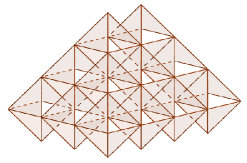
Figure 2: $\Xi_{4}^{(n)}$

If $p\in\Xi_{4}^{(n)}$, the forms $D_{j}\omega(p)=\omega_{j}(p)$ are on $\Xi_{4}^{(n+1)}$ for all $j$, hence

$$D:\quad\Xi_{4}^{(n)}\to\Xi_{4}^{(n+1)},$$

with $D=(D_{1},D_{2},D_{3},D_{4})$. Since all functions in the HM eq.(1) are of the form $\tau_{ij}(p)=D_{i}D_{j}\tau(p)$, they are on $\Xi_{4}^{(n+2)}$ if $p\in\Xi_{4}^{(n)}$. Moreover the six functions $\tau_{ij}(p)$ in (1) are at the six corners of the octahedron whose center is at $p$. Hence the HM eq. determines relations among functions on $\Xi_{4}^{(n+2)}$. In other words solutions of the HM eq. are different if they are on different hyperplanes. We mention that this is a result of the fact that the HM eq. is a Plücker relation.

Let us define $\omega^{(n)}$ by

$$\omega^{(n)}(p):\ \Xi_{4}^{(n)}\ \to\ \mathbb{C},\qquad n\in\mathbb{Z}$$

when $p\in\Xi_{4}^{(n)}$. We then naturally obtain a graded algebra

$$\bigoplus_{n\in\mathbb{Z}}\ \mathbb{C}\ \omega^{(n)}$$ (12)

on which $d_{B}$ acts by

$$d_{B}^{(n)}:\quad\omega^{(n)}\to\omega^{(n+1)}.$$ (13)

2.2.2 3 dimensional ‘difference’ forms

From Fig.2 we can see that the lattice space $\Xi_{4}^{(n+2)}$ consists of parallel planes, each filled by triangles of octahedra, as illustrated in Fig.3. If we fix the direction of the planes parallel to the direction of $-p_{4}$, we can specify them by the values of $t:=p_{1}+p_{2}+p_{3}$. Such a plane is defined by

$$\Xi_{3}^{(t,n+2)}:=\Big{\{}(p_{1},p_{2},p_{3})\in\mathbb{Z}^{3}\Big{|}p_{1}+p_{2}+p_{3}=t\in\mathbb{Z},\ (p_{1},p_{2},p_{3},p_{4})\in\Xi_{4}^{(n+2)}\Big{\}},$$

$$\bigcup_{t\in\mathbb{Z}}\Xi_{3}^{(t,n+2)}=\Xi_{4}^{(n+2)}.$$

Since $n+2\ (=p_{1}+p_{2}+p_{3}+p_{4})=t+p_{4}$ is fixed, the planes are perpendicular to the direction of $-p_{4}$.

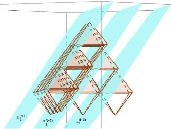
Figure 3: $\Xi_{3}^{(t,n+2)}$

We denote a point on $\Xi_{3}^{(t,n+2)}$ by $\mbox{\boldmath$p$}=(p_{1},p_{2},p_{3})\in\mathbb{Z}^{3}$. Corresponding to $d_{B}$ of (13) we define the 3 dimensional exterior ‘difference’ operator $d_{T}$ by

$$d_{T}\omega(\mbox{\boldmath$p$})=\sum_{a=1}^{3}D_{a}\omega(\mbox{\boldmath$p$})\wedge dp_{a},\qquad^{\forall}\omega(\mbox{\boldmath$p$}):\ \Xi_{3}^{(t,n+2)}\to\mathbb{C},$$

which we call the shift operator. Since, similar to the 4 dimensional case, $\omega(\mbox{\boldmath$p$})$ and $D_{a}\omega(\mbox{\boldmath$p$})$ are on different planes, we define graded forms of degree $t$ by $\omega[t]$ when $\mbox{\boldmath$p$}\in\Xi_{3}^{(t,n+2)}$. The graded algebra

$$\bigoplus_{t\in\mathbb{Z}}\mathbb{C}\omega[t]$$

is generated by

$$d_{T}^{[t]}:\ \ \omega[t]\to\omega[t+1].$$ (14)

3 Dynamical feature of the HM eq.

Based on the geometrical structure of the HM eq. we studied in the previous section, we discuss dynamical feature of the HM eq. in this section.

3.1 Linear Bäcklund transformation

In order to study dynamical feature of the HM eq. we consider a pair of 4 dimensional ‘difference’ 2-forms [2]

$$F:=\sum_{i,j=1}^{4}F_{ij}dp_{i}\wedge dp_{j}, F_{ij}(p)=a_{ij}\tau_{ij}(p),$$ (15)

$$\tilde{F}:=\sum_{i,j=1}^{4}\tilde{F}_{ij}dp_{i}\wedge dp_{j}, \tilde{F}_{ij}(p)={}^{*}a_{ij}\tau_{ij}(p)$$ (16)

with ${}^{*}a_{ij}=\sum_{kl}\epsilon_{ijkl}a_{kl}$, where $\epsilon_{ijkl}$ is the Levi-Civita symbol. We can easily check that each of the followings [16]

$$\det F_{ij}=0,\qquad\det\tilde{F}_{ij}=0$$ (17)

is equivalent to the HM eq. (1). By this reason we call $F$ of (15) the HM 2-form in this paper.

Let us consider, for any $\tau(p)$ and $\sigma(p)$, the following forms

$$\tilde{F}\wedge{\rm d_{B}}\sigma = \sum_{j,k,l}{}^{*}a_{kl}\tau_{kl}\sigma_{j}dp_{k}\wedge dp_{l}\wedge dp_{j}=\sum_{i,j}\tilde{F}_{ij}\sigma_{j}\ ^{*}dp_{i},$$

$$d_{B}(\tilde{F}\wedge{\rm d_{B}}\sigma) = \sum_{i,j}a_{ij}{}^{*}\tau_{j}\sigma_{ij}dp_{i}\wedge{{}^{*}dp_{i}}=:\sum_{i,j}G_{ij}{}^{*}\tau_{j}\delta_{i},$$

where we used the notation ${}^{*}dp_{i}:=\epsilon_{ijkl}dp_{j}\wedge dp_{k}\wedge dp_{l}$ and $\sum_{kl}\epsilon_{ijkl}{}^{*}a_{kl}\tau_{ikl}=a_{ij}{}^{*}\tau_{j}$. If we require $\tilde{F}\wedge{\rm d_{B}}\sigma=0$, it is compatible iff $d_{B}(\tilde{F}\wedge{\rm d_{B}}\sigma)=0$, or equivalently

$$\sum_{j}\tilde{F}_{ij}\sigma_{j}=0, \qquad i=1,2,3,4$$

$$\Updownarrow$$

$$\sum_{j}G_{ij}{}^{*}\tau_{j}=0, \qquad i=1,2,3,4.$$ (19)

Now suppose $\tau^{(0)}(p)$ is a solution of the HM eq. (1). If it is substituted to $\tilde{F}$ in (3.1), we can solve the linear equation for $\sigma$, because $\tilde{F}$ satisfies (17). Let us denote by $\tau^{(1)}(p)$ the solution of (3.1) which is just obtained dependent on $\tau^{(0)}$. Then we can substitute $\tau^{(1)}$ into $G$ of (19). Because (3.1) and (19) are the same equation, the equation (19) for $\tau$ has certainly solution. This means $\det G$ must vanish, so that, by (17) again, $\tau^{(1)}(p)$ is a solution of the HM eq..

As $\tau^{(1)}(p)$ is substituted the linear equation (19) has solutions other than $\tau^{(0)}$ in general. Let $\tau^{(2)}$ be one of them which is independent from $\tau^{(0)}$. $\tau^{(2)}$ is again a solution of the HM eq., so that we can substitute it to (3.1) to find $\tau^{(3)}$, and so on. Here we must mention that if the initial function $\tau^{(0)}(p)$ is on $\Xi_{4}^{(n)}$, the solution $\tau^{(1)}(p)$ is on $\Xi_{4}^{(n+1)}$. We can repeat this procedure and obtain a sequence of the Bäcklund transformation [17]

$$\tau^{(0)}\quad\smash{\mathop{\hbox to28.45274pt{\rightarrowfill}}\limits^{{\rm d_{B}^{(0)}}}}\quad\tau^{(1)}\quad\smash{\mathop{\hbox to28.45274pt{\rightarrowfill}}\limits^{{\rm d_{B}^{(1)}}}}\quad\tau^{(2)}\quad\smash{\mathop{\hbox to28.45274pt{\rightarrowfill}}\limits^{{\rm d_{B}^{(2)}}}}\quad\tau^{(3)}\quad\smash{\mathop{\hbox to28.45274pt{\rightarrowfill}}\limits^{{\rm d_{B}^{(3)}}}}\quad\cdots$$ (20)

If we choose another solution of the HM eq. for the initial function $\tau^{(0)}$, we should have different series of solutions. In fact, in the string theory, we can add loops of closed strings so that the world sheet increases holes as is depicted in the Fig.1. There is also a vertex operator which substitutes a D-brane, so that the world sheet is attached to a boundary [18]. All such variations change the topology of the state $|G\rangle$, and corresponds to different initial solution $\tau^{(0)}$ of the HM eq.. If we denote the complex (20) by ${\mathcal{B}T}_{G}$ corresponding to the state $|G\rangle$, we will find a family of complexes of the Bäcklund transformation.

3.2 Dynamical evolution

In this subsection we fix the hyperplane $\Xi_{4}^{(n+2)}$, hence we simply denote $\Xi_{3}^{(t,n+2)}$ by $\Xi_{3}^{[t]}$, and study behavior of a particular solution of the HM eq. For this purpose we rewrite the HM 2-form by using the operator $d_{T}$ of (14) as

$$F=\sum_{i,j=1}^{4}F_{ij}dp_{i}\wedge dp_{j}=d_{T}\left(F_{4}(p)dp_{4}+\sum_{b=1}^{3}F_{b}(p)dp_{b}\right)$$

and see that the six components $F_{ij}$ split into two parts

$$d_{T}F_{4}(p) = \sum_{a=1}^{3}F_{a4}(\mbox{\boldmath$p$})dp_{a},$$ (21)

$$d_{T}\sum_{b=1}^{3}F_{b}(p)dp_{b} = \sum_{b,c=1}^{3}F_{bc}(\mbox{\boldmath$p$})dp_{b}\wedge dp_{c},$$ (22)

corresponding to 3 dimensional 1-form and 2-form, respectively.

Let us denote by $\tilde{S}_{j}$ and $S_{j}$ the triangles in an octahedron which are perpendicular to $p_{j}$ and parallel each other. Then we can see that $\{F_{a4}\}$ and $\{F_{bc}\}$ form triangles

$$\tilde{S}_{4}:=\Big{(}\tau_{14},\tau_{24},\tau_{34}\Big{)},\qquad S_{4}:=\Big{(}\tau_{23},\tau_{31},\tau_{12}\Big{)},$$

which are perpendicular to $p_{4}$. We denote the octahedron, which consists of these triangles, by ${\mathcal{O}}=(\tilde{S}_{4},S_{4})$, as illustrated in Fig.4.

Figure 4:

From Fig.3 we see that every octahedron is put between two nearest planes, such that two parallel triangles are on each plane. In fact the triangle $\tilde{S}_{4}$ is on $\Xi_{3}^{[t+1]}$ and $S_{4}$ is on $\Xi_{3}^{[t+2]}$ if $\tau(\mbox{\boldmath$p$})$ is on $\Xi_{3}^{[t]}$. Define ${\mathcal{O}}[t]=(\tilde{S}_{4}[t+1],S_{4}[t+2])$ with

$$\tilde{S}_{4}[t+1] = \Big{(}\tau_{14}[t+1],\tau_{24}[t+1],\tau_{34}[t+1]\Big{)},$$

$$S_{4}[t+2] = \Big{(}\tau_{23}[t+2],\tau_{31}[t+2],\tau_{12}[t+2]\Big{)}$$

and let $\{{\mathcal{O}}\}[t]$ be all set of octahedra put between $\Xi_{3}^{[t+1]}$ and $\Xi_{3}^{(t+2)}$. Then the procedure to solve initial value problem is to determine the following sequence

$$\{{\mathcal{O}}\}\quad\stackrel{{\scriptstyle d_{T}}}{{\longrightarrow}}\quad\{{\mathcal{O}}\}[1]\quad\stackrel{{\scriptstyle d_{T}}}{{\longrightarrow}}\quad\{{\mathcal{O}}\}[2]\quad\stackrel{{\scriptstyle d_{T}}}{{\longrightarrow}}\quad\{{\mathcal{O}}\}[3]\quad\stackrel{{\scriptstyle d_{T}}}{{\longrightarrow}}\quad\cdots$$ (23)

when information $\{{\mathcal{O}}\}$ at initial time $t=0$ is given.

3.3 Deterministic rule for the flow of information

We want to know how information on $\{{\mathcal{O}}\}$ transfers to other octahedra as $t$ increases. The HM eq determines a relation between $\tilde{S}_{4}$ and $S_{4}$. But it does not tell us how the information of $\tilde{S}_{4}$ transfers to $S_{4}[1]$. In order to solve an initial value problem we must know some deterministic rules which decide uniquely the local flow of information. In this subsection we set up a rule for the flow of information in an octahedron.

Let us consider two lattice points $p$ and $p^{\prime}$ on $\Xi_{4}$ which are separated by

$$p^{\prime}-p=m\in\mathbb{Z}^{4}.$$

If they are on the same hyperplane $\Xi_{4}^{(n)}$, the separation $m$ must satisfy

$$m_{1}+m_{2}+m_{3}+m_{4}=0.$$ (24)

If $p$ and $p^{\prime}$ are neighbor of an octahedron,

$$m=\delta_{i}-\delta_{j},\qquad i\neq j$$ (25)

corresponding to the edge parallel to the vector $p_{i}-p_{j}$. There will be many possible routs along which information can transfer between two points $p$ and $p^{\prime}$ fixed arbitrary. Since an addition of a path of the type (25) does not change the condition (24), any routs can connect $p$ and $p^{\prime}$ as long as they are connected by edges of octahedra.

When we decide the rule of transfer of information we must keep in mind the following items:

• Information at $p+\delta_{i}+\delta_{j}$ is transfered properly to $p^{\prime}+\delta_{k}+\delta_{l}$ if all operators corresponding to all possible routs $\{r\}$ change $\tau_{ij}(p)$ to $\tau_{kl}(p^{\prime})$ uniquely.

  $$D_{r}(ij,kl)_{p,p^{\prime}}:\ \ \tau_{ij}(p)\stackrel{{\scriptstyle r}}{{\longrightarrow}}\tau_{kl}(p^{\prime}),\qquad\forall r.$$

• Our system is deterministic if a rule of transfer of information is fixed along edges of an octahedron, and is the same for all octahedra.

• The system is integrable if this rule is sufficient to predict the values of $\tau$ on $\Xi_{3}^{[t]}$ for all $t$ when the values on $\Xi_{3}^{(0)}$ are given arbitrary.

There are 12 edges in an octahedron ${\mathcal{O}}$. Every object $\tau_{ij}$ at a corner has connections to its four neighbors but no direct connection to its diagonal one. Since we are interested in a flow of information from one corner to another of ${\mathcal{O}}$, we must decide direction (hence a rule) of the flow. In other words we fix the order of points in ${\mathcal{O}}$. A natural way is the cyclic ordering of suffixes, i.e.,

$$1<2<3<4<1<2<3.$$ (26)

We notice in Fig. 4 that every pair of corners connected by an edge have a common suffix, like $(\tau_{14},\tau_{12})$. Therefore we define the direction of transfer by

$$D(ij,ik):\tau_{ij}\longrightarrow\tau_{ik},\qquad{\it iff}\quad k<i<j.$$ (27)

For example, $D(34,24)$ is possible because $3<4<2$, but $D(24,12)$ is not possible because $4<2<1$ is not compatible with (26), etc. In this way we can define uniquely the directions which are necessary to connect all objects in ${\mathcal{O}}$. In Fig.5 $(a)$ the directions allowed by this rule (27) are shown by arrows. If we project the diagram along $p_{3}$ we have Fig.5 $(b)$.

Figure 5:

The action of $D(kl,ij)$ is to remove punctures at $z_{i}$ and $z_{j}$ from $|G\rangle$ and insert other punctures at $z_{k}$ and $z_{l}$. It will be convenient to represent this action explicitly by means of the operators:

$$D(ij,kl)=D_{k}D_{l}D_{j}^{-1}D_{i}^{-1}.$$ (28)

We can easily check the rule of product,

$$D(ij,kl)\circ D(kl,mn)=D(ij,mn).$$

From

$$D(ij,kl)\circ D(kl,ij)=D(ij,ij)=id$$

we see that $D(ij,kl)$ is an isomorphism.

Since corners connected by an edge have a common suffix, (28) simplifies

$$D(ij,ik)=D_{k}D_{j}^{-1}$$

whereas the morphism connecting the diagonals of an octahedron can be obtained by a product of morphisms, for instance, like

$$D(23,24)\circ D(24,14)=D(23,14)=D_{2}D_{3}D_{4}^{-1}D_{1}^{-1}.$$

3.4 Transfer of information along a chain of octahedra

In this subsection we want to see how information flows along a chain of octahedra. Let us denote by ${\mathcal{O}}(p)=(\tilde{S}_{4}(p),S_{4}(p))$ the octahedron whose center is at $p\in\Xi_{4}^{(n)}$. There are three octahedra which share three edges of the triangle $S_{4}(p)$. Since these three neighbors are on the same hyperplane $\Xi_{4}^{(n+2)}$ their centers must be at $p+\delta_{1}-\delta_{4},\ p+\delta_{2}-\delta_{4},\ p+\delta_{3}-\delta_{4}$, respectively. Let ${\mathcal{O}}(p)[1]$ be one of them, say ${\mathcal{O}}(p+\delta_{3}-\delta_{4})$. Then these octahedra are connected as illustrated in Fig.6, where we use the abbreviations:

$$\tilde{S}_{4}=(X,Y,Z)=\Big{(}\tau_{14},\tau_{24},\tau_{34}\Big{)},\quad S_{4}=(X^{\prime},Y^{\prime},Z^{\prime})=\Big{(}\tau_{23},\tau_{31},\tau_{12}\Big{)}.$$

Figure 6:

For the information of ${\mathcal{O}}$ to transfer to its neighbor ${\mathcal{O}}[1]$ properly, we must impose the following conditions:

$$\tau_{14}[1]=\tau_{13},\qquad\tau_{24}[1]=\tau_{23}.$$ (29)

Repeating this procedure we can define a chain of octahedra by

$${\mathcal{O}}(p)[t]={\mathcal{O}}(p+t\delta_{3}-t\delta_{4}),\quad t\in\mathbb{Z}.$$ (30)

We recall that $\tilde{S}_{4}(p)$ is on $\Xi_{3}^{[t+1]}$ and $S_{4}(p)$ is on $\Xi_{3}^{(t+2)}$, if $p_{1}+p_{2}+p_{3}=t$. Because $d_{T}$ transfers information on $\Xi_{3}^{[t]}$ to $\Xi_{3}^{[t+1]}$ we see that the information on ${\mathcal{O}}$ can be transfered along the chain of octahedra

$${\mathcal{O}}\smash{\mathop{\hbox to28.45274pt{\rightarrowfill}}\limits^{{\rm d}_{T}}}{\mathcal{O}}[1]\smash{\mathop{\hbox to28.45274pt{\rightarrowfill}}\limits^{{\rm d}_{T}}}{\mathcal{O}}[2]\smash{\mathop{\hbox to28.45274pt{\rightarrowfill}}\limits^{{\rm d}_{T}}}{\mathcal{O}}[3]\smash{\mathop{\hbox to28.45274pt{\rightarrowfill}}\limits^{{\rm d}_{T}}}\cdots.$$ (31)

if the connection conditions (29) are satisfied at every site of connection. This is certainly compatible with (23), and explains the local flow of information.

4 View from the theory of category

We are now ready to summarize our result in the previous section in terms of the category theory.

4.1 Triangulated category

We have pointed out in our previous paper [2] a possible explanation of the flow of information by means of the triangulated category. In order to see this correspondence more in detail let us first recall the axioms of triangulated category [19, 20].

Definition

Let ${\mathcal{D}}$ be an additive category, $X,Y,Z,X^{\prime},Y^{\prime},Z^{\prime}$ be objects and $u,v,w$ be morphisms of ${\mathcal{D}}$. The structure of a triangulated category on ${\mathcal{D}}$ is defined by the shift functor $T$ and the class of distinguished triangles satisfying the following axioms:

1. $(1)$Any triangle of the form

   $$X\stackrel{{\scriptstyle\rm id}}{{\longrightarrow}}X\longrightarrow 0\longrightarrow T(X)$$

   is in the class of distinguished triangles.
   $(2)$ Any triangle isomorphic to a distinguished triangle is distinguished.
   $(3)$ Any morphism $u:X\rightarrow Y$ can be completed to a distinguished triangle

   $$X\stackrel{{\scriptstyle u}}{{\longrightarrow}}Y\longrightarrow C(u)\longrightarrow T(X)$$

   by the object $C(u)$ obtained by morphism $u$.

2. The triangle

   $$X\stackrel{{\scriptstyle u}}{{\longrightarrow}}Y\stackrel{{\scriptstyle v}}{{\longrightarrow}}Z\stackrel{{\scriptstyle w}}{{\longrightarrow}}T(X)$$

   is a distinguished triangle if and only if

   $$Y\stackrel{{\scriptstyle v}}{{\longrightarrow}}Z\stackrel{{\scriptstyle w}}{{\longrightarrow}}T(X)\stackrel{{\scriptstyle-T(u)}}{{\longrightarrow}}T(Y)$$

   is a distinguished triangle.

3. Suppose there exists a commutative diagram of distinguished triangles,

   $$\hskip 1.42262ptX\hskip 1.42262pt\longrightarrow Y\hskip 1.42262pt\longrightarrow\hskip 1.42262ptZ\hskip 2.84526pt\longrightarrow T(X)$$

   $$u \downarrow\hskip 18.49428ptv\downarrow\hskip 71.13188pt\downarrow T(u)$$

   $$X^{\prime}\longrightarrow Y^{\prime}\longrightarrow Z^{\prime}\longrightarrow T(X^{\prime}).$$

   Then this diagram can be completed to a commutative diagram by a (not necessarily unique) morphism $w:Z\rightarrow Z^{\prime}$.

4. (the octahedron axiom) Let $X\stackrel{{\scriptstyle u}}{{\longrightarrow}}Y\stackrel{{\scriptstyle v}}{{\longrightarrow}}Z$ be a triangle. Then the following commutative diagram holds:

   (32)

Comparing this set of axioms Tr1 $\sim$ Tr4 with our arguments in §3.3 and §3.4, we naturally find the following correspondence:

$$\begin{array}[]{ccc}objects&\longleftrightarrow&\tau\ functions,\cr morphism&\longleftrightarrow&D(ij,ik),\cr T:A\to T(A)&\longleftrightarrow&d_{T}:A\to A[1],\cr octahedron\ axiom&\longleftrightarrow&flow\ diagram\ Fig.\ref{fig6}.\end{array}$$ (33)

For example there are flows of information which start from $A\in(X,Y,Z)$ and then end at $A[1]\in\Big{(}X[1],Y[1],Z[1]\Big{)}$ as

$$\begin{array}[]{ccccccc}X&\to&Y&\to&Z&\to&X[1],\cr X&\to&Y&\to&Z^{\prime}&\to&X[1],\cr X&\to&Z&\to&Y^{\prime}&\stackrel{{\scriptstyle id}}{{\to}}&X[1],\cr Y&\to&Z&\to&X^{\prime}&\stackrel{{\scriptstyle id}}{{\to}}&Y[1],\cr Z&\to&Y^{\prime}&\to&X^{\prime}&\to&Z[1].\cr\end{array}$$ (34)

They are all compatible with the axioms as we can check easily. Here $id$’s in (34) owe to the condition (29). Via these routs information in ${\mathcal{O}}$ can transfer to ${\mathcal{O}}[1]$. Let us denote the triangulated category (33) as ${\mathcal{H}M}_{G}^{(n)}$ in this paper. The suffix $(n)$ is to remind that a solution of the HM eq is given separately for each lattice space $\Xi_{4}^{(n)}$, while the suffix $G$ is to remind that the solution is dependent on the initial state $|G\rangle$.

4.2 The category theory of global behavior

From above arguments we see that the objects of the category ${\mathcal{H}M}_{G}^{(n)}$

$${\rm Ob}({\mathcal{H}M}_{G}^{(n)})=\{\tau^{(n)}_{ij}(p)\ \Big{|}\ p\in\Xi_{4}^{(n)}\}$$

are nothing but a solution of the HM eq (1), which we denote as

$${\mathcal{H}M}_{G}^{(n)}\simeq\tau_{G}^{(n)}$$ (35)

when $|G\rangle$ is given.

On the other hand we learned in §3.1 that a series of the Bäcklund transformations forms a complex ${\mathcal{B}T}_{G}$ of solutions of the HM eq associated to the state $|G\rangle$, i.e.,

$$d_{B}:\ \tau_{G}^{(n)}\ \to\ \tau_{G}^{(n+1)}.$$

If we combine this with the result (35) we obtain

$${\mathcal{B}T}_{G}=\Big{\{}\{{\mathcal{H}M}_{G}^{(n)}\}_{n\in\mathbb{Z}},\ d_{B}\Big{\}}.$$

Therefore ${\mathcal{B}T}_{G}$ is a category of categories and $d_{B}$ is a functor.

Moreover, as we mentioned in §3.1, the change of the state $|G\rangle$

$$|G\rangle\to|G^{\prime}\rangle={\mathcal{F}}|G\rangle.$$

will generate a different complex ${\mathcal{B}T}_{G^{\prime}}$ of the Bäcklund transformations. Therefore we obtain another functor

$${\mathcal{F}}:\ {\mathcal{B}T}_{G}\ \to\ {\mathcal{B}T}_{G^{\prime}}.$$

We have thus found various type of categories which are related from each other. Among others our interpretation of the information flow of the HM eq. by means of the triangulated category is the most fundamental. However the correspondence of the flow with the triangulated category seems not quite right by two reasons.

1. An addition of objects is no longer an object in general, because our objects are solutions of a nonlinear equation. Although most of studies of triangulated category have been based on additive categories in mathematics, the above axioms themselves do not use the notion of additivity. Therefore nonadditive nature of our theory will not cause any problem.

2. Second reason is that we have not yet defined null object 0, which appears in the first axiom Tr1. This is the main subject of this paper which we are going to discuss in the following section.

5 Localization and singularity confinement

It is well known that a localization of a triangulated category is also a triangulated category. We show in this section that the singularity confinement of a rational map obtained from the $\tau$ function of the HM eq. can be described in terms of the localization of the triangulated category.

5.1 Reduction of the lattice space

We have studied difference geometry of 4 and 3 dimensions in §2. Our concern in this section is a 2 dimensional lattice space.

If we fix $n=p_{1}+p_{2}+p_{3}+p_{4}-2$ and $t=p_{1}+p_{2}+p_{3}$ we are left with 2 dimensional lattice space, which we parameterize by

$$q=p_{1}+p_{2},\qquad j:=p_{2}-p_{1}.$$

Like the higher dimensional lattice cases we define 2 dimensional lattice space

$$\Xi_{2}^{(q,t,n+2)}:=\Big{\{}(p_{1},p_{2})\in\mathbb{Z}^{2}\Big{|}p_{1}+p_{2}=q\in\mathbb{Z},\ (p_{1},p_{2},p_{3})\in\Xi_{3}^{(t,n+2)}\Big{\}},$$

$$\bigcup_{q\in\mathbb{Z}}\Xi_{2}^{(q,t,n+2)}=\Xi_{3}^{(t,n+2)}$$

and the exterior difference operator d_Q by

$${\rm d}_{Q}\tau(\mbox{\boldmath$p$})=D_{1}\tau(\mbox{\boldmath$p$})dp_{1}+D_{2}\tau(\mbox{\boldmath$p$})dp_{2},$$

which displaces the lattice space

$$D:\Xi_{2}^{(q,t,n+2)}\to\Xi_{2}^{(q+1,t,n+2)}.$$

Because $t=q+p_{3}$, we can fix $p_{3}$ instead of $t$. In this frame of coordinate, the change of $t$ is exactly the same with the change of $q$. We recall that the diagram Fig.6 (b) was the projection Fig.6 (a) along $p_{3}$. Since $j=p_{2}-p_{1}\in\mathbb{Z}$ is still free we denote $\tau^{[t]}_{j}:=\tau(\mbox{\boldmath$p$})$ and consider the lattice space

$$\Big{\{}(j,t)\in\mathbb{Z}^{2}\Big{|}\Delta t=\Delta q,p_{2}-p_{1}=j\in\mathbb{Z},(p_{1},p_{2})\in\Xi_{2}^{(q,t,n+2)}\Big{\}}.$$

In our previous section we discussed the transfer of information along the chain of octahedra. We now extend the study to consider a transfer of information of many octahedra linked along a line in the $j$ direction.

We have to mention that the connection condition (29) is already taken into account in this expression. Moreover the projection along $p_{3}$ enforces degeneration of $Z^{\prime}[t]$ in ${\mathcal{O}}[t]$ and $Z[t+2]$ in ${\mathcal{O}}[t+2]$. Therefore the shift operation d_T brings $\tilde{S}_{4}$ directly to $\tilde{S}_{4}[1]$, so that $\tau_{j}^{[t]}$ is determined uniquely for all $t$ and $j$ as we can see in the Fig.7.

Figure 7:

In the theory of KP hierarchy it is known that we can either truncate the function $\tau_{j}^{[t]}$, or impose periodicity in the direction of $j$ at any value, with no violation of integrability. For example we can impose

$$\tau_{j+d}^{[t]}=\tau_{j}^{[t]}$$ (36)

to obtain a reduced map of $d$ dimension. In this case it is more convenient to consider

$$\mbox{\boldmath$\tau$}^{[t]}=(\tau^{[t]}_{0},\tau^{[t]}_{1},\tau^{[t]}_{2},\tau^{[t]}_{3},...,\tau^{[t]}_{d-1}),$$

instead of a triangle $\tilde{S}_{4}$ of each octahedron separately. When $d=3$, the chain of Fig.7 becomes a chain of triangles.

5.2 Localization of a triangulated category

The theory of triangulated category tells us that, if there is a null system, the theory can be localized such that the localized theory again satisfies the axioms of triangulated category [19, 21]. A null system ${\mathcal{N}}\subset{\mathcal{T}}$ of the triangulated category ${\mathcal{T}}$ is a set of objects defined by

1. $0\in{\mathcal{N}}$.

2. $Z\in{\mathcal{N}}$ if $X,Y\in{\mathcal{N}}$ and $X\to Y\to Z\to X[1]$ is a distinguished triangle.

3. $X[1]\in{\mathcal{N}}$ iff $X\in{\mathcal{N}}$.

For any triangulated category ${\mathcal{T}}$ and a null system ${\mathcal{N}}\subset{\mathcal{T}}$, we define a multiplicative system by

$$S({\mathcal{N}}):=\{g|X\stackrel{{\scriptstyle g}}{{\to}}Y\to Z\to X[1],\ X,Y\in{\mathcal{T}},\ Z\in{\mathcal{N}}\}.$$

Then the localization is defined by the functor ${\mathcal{T}}\to{\mathcal{T}}/S({\mathcal{N}})$. The following theorem is known in the theory of triangulated category:

Theorem

${\mathcal{T}}/S({\mathcal{N}})$ is again a triangulated category whose null object is 0 itself.

Therefore, in order to discuss the localization of our system we must know a null system of our triangulated category. Our objects are solutions $\{\tau_{ij}\}$ of the HM eq. which are assigned at corners of each octahedron. They are generically finite, because the $\tau$ functions are defined by the ratios (5) of correlation functions such that the zeros of correlation functions cancel from each other.

As we explained in §2.1 the correlation functions $\{\Phi_{ij}\}$ vanish by themselves when two punctures encounter on the Riemann surface. It is, however, important to notice that, when the correlation functions $\Phi(p,z;G)$ and $\Phi(p,z;0)$ vanish simultaneously, the cancellation of their zeros does not mean the value of their ratio being definite. Let $\lambda(p)$ be the ratio of the correlation functions at the point where they vanish, i.e.

$$\lambda(p):=\left\{\left.{\Phi(p,z;G)\over\Phi(p,z;0)}\right|\Phi(p,z;G)=\Phi(p,z;0)=0\right\},$$ (37)

then $\lambda(p)$ is indeterminate in general, hence can take any value. Since zero is not excluded in (37) we call the zero of $\lambda(p)$ the null object and denote by 0, i.e.,

$$0\in\lambda(p).$$

We now focus our attention to this subtle object in the following discussion and show how the localization of triangulated category resolves the subtlety.

The localization of our system will be introduced by considering rational maps of the $\tau$ functions. To be specific we consider some reduced flow diagrams of Fig.7 which satisfy the condition (36). In particular we study in detail rational maps defined by the following variables:

$$x_{j}^{[t]}=\left\{\begin{array}[]{cll}\displaystyle{{\tau_{j+\epsilon+1}^{[t]}\tau_{j-\epsilon}^{[t+1]}\over\tau_{j+1}^{[t]}\tau_{j}^{[t+1]}}},&\quad j,\epsilon=1,2,3,...,d,&\quad{\rm LV},\cr&&\cr\displaystyle{{\tau_{j+1}^{[t]}\tau_{j-\epsilon}^{[t+1]}\over\tau_{j}^{[t]}\tau_{j+1-\epsilon}^{[t+1]}}},&\quad j,\epsilon=1,2,3,...,d,&\quad{\rm KdV}.\cr\end{array}\right.$$ (38)

The maps which are obtained by the new variables LV and KdV are called the Lotka-Volterra map and the Korteweg-de Vries map, respectively [22, 23].

An important feature of the variables (38) is that they are invariant under the local gauge transformation of $\tau_{j}^{[t]}$

$$g:\ \tau_{j}^{[t]}\to\exp\left(\int^{t}\nu(t^{\prime},j)dt^{\prime}+\int^{j}\mu(t,j^{\prime})dj^{\prime}\right)\tau_{j}^{[t]},$$ (39)

where $\nu(t,j)$ and $\mu(t,j)$ are arbitrary functions. For example, we can write the right hand side of (38) as

$$x_{j}^{[t]}=\left\{\begin{array}[]{cll}\displaystyle{{\Phi_{j+\epsilon+1}^{[t]}(p,z)\Phi_{j-\epsilon}^{[t+1]}(p,z)\over\Phi_{j+1}^{[t]}(p,z)\Phi_{j}^{[t+1]}(p,z)}},&\quad j,\epsilon=1,2,3,...,d,&\quad{\rm LV},\cr&&\cr\displaystyle{{\Phi_{j+1}^{[t]}(p,z)\Phi_{j-\epsilon}^{[t+1]}(p,z)\over\Phi_{j}^{[t]}(p,z)\Phi_{j+1-\epsilon}^{[t+1]}(p,z)}},&\quad j,\epsilon=1,2,3,...,d,&\quad{\rm KdV}.\cr\end{array}\right.$$ (40)

This follows from the fact that the denominator of $\tau_{j+k}^{[t+u]}(p)$ is given by

$$\Phi_{j+k}^{[t+u]}(p,z,0)=(z_{1}-z_{2})^{(p_{1}-k)(p_{2}+k)}(z_{3}-z_{4})^{(p_{3}+u)(p_{4}-u)}$$

so that all denominators of $\tau$ functions in (38) are eliminated exactly from the expression.

We notice that we can not distinguish a change of $\lambda(p)$ in (37) with the gauge transformation

$$g:\lambda(p)\longrightarrow\lambda^{\prime}(p).$$ (41)

This means that, if $\Lambda(\infty)$ is the set of all possible $\lambda(p)$, i.e.,

$$\Lambda(\infty):=\Big{\{}\lambda(p)\Big{|}p\in\Xi_{4}^{(n+2)}\Big{\}}.$$ (42)

$\Lambda(\infty)$ is invariant under the gauge transformation.

Now suppose that $\tau_{j}^{[t+1]}$ (or $\tau_{j+1-\epsilon}^{[t+1]}$ in the KdV case) in the denominator of $x_{j}^{[t]}$ in (38) is the null object, hence takes the value zero. Then $x_{j}^{[t]}$ and also $x_{j-1}^{[t+1]}$ diverge while all components of $\mbox{\boldmath$x$}^{[t+u]}$ with $u\geq 2$ are finite, as far as other $\tau$ functions are finite. This owes to the fact that the same $\tau$ function does not propagate beyond two steps. There is no way to determine the values of $\tau^{[t+1]}$’s because the null object is invariant under the gauge (41), i.e.,

$$g:0\longrightarrow g0=0.$$

In other words the null object is transfered to an indeterminate object,

$$d_{T}:0\longrightarrow\lambda(p).$$ (43)

which is an element of $\Lambda(\infty)$. It should be emphasized that $\Lambda(\infty)$ does not appear in the localized theory, because the localized variables $x_{j}^{[t]}$’s are gauge invariant. Thus we are strongly suggested to identify $\Lambda(\infty)$ with the null system ${\mathcal{N}}$ of our map

$${\mathcal{N}}\sim\Lambda(\infty).$$ (44)

Our argument in the rest of this paper will be devoted to support this conjecture.

5.3 Singularity confinement

To proceed our argument further we consider the case $d=3$ and $\epsilon=1$ in (38) for simplicity. Then the HM eq. becomes the following rational maps,

$${\rm LV\ map} \qquad\left\{\begin{array}[]{c}x_{1}^{[t+1]}=x_{1}^{[t]}\displaystyle{{1-x_{2}^{[t]}+x_{2}^{[t]}x_{3}^{[t]}\over 1-x_{3}^{[t]}+x_{3}^{[t]}x_{1}^{[t]}}},\\ x_{2}^{[t+1]}=x_{2}^{[t]}\displaystyle{{1-x_{3}^{[t]}+x_{3}^{[t]}x_{1}^{[t]}\over 1-x_{1}^{[t]}+x_{1}^{[t]}x_{2}^{[t]}}},\\ x_{3}^{[t+1]}=x_{3}^{[t]}\displaystyle{{1-x_{1}^{[t]}+x_{1}^{[t]}x_{2}^{[t]}\over 1-x_{2}^{[t]}+x_{2}^{[t]}x_{3}^{[t]}}},\\ \end{array}\right.$$ (48)

$${\rm KdV\ map} \qquad\left\{\begin{array}[]{c}x_{1}^{[t+1]}=x_{1}^{[t]}\displaystyle{{1+x_{1}^{[t]}x_{3}^{[t]}+x_{1}^{[t]}x_{2}^{[t]}(x_{3}^{[t]})^{2}\over 1+x_{1}^{[t]}x_{2}^{[t]}+(x_{1}^{[t]})^{2}x_{2}^{[t]}x_{3}^{[t]}}},\\ x_{2}^{[t+1]}=x_{2}^{[t]}\displaystyle{{1+x_{1}^{[t]}x_{2}^{[t]}+(x_{1}^{[t]})^{2}x_{2}^{[t]}x_{3}^{[t]}\over 1+x_{2}^{[t]}x_{3}^{[t]}+x_{1}^{[t]}(x_{2}^{[t]})^{2}x_{3}^{[t]}}},\\ x_{3}^{[t+1]}=x_{3}^{[t]}\displaystyle{{1+x_{2}^{[t]}x_{3}^{[t]}+x_{1}^{[t]}(x_{2}^{[t]})^{2}x_{3}^{[t]}\over 1+x_{1}^{[t]}x_{3}^{[t]}+x_{1}^{[t]}x_{2}^{[t]}(x_{3}^{[t]})^{2}}}.\\ \end{array}\right.$$ (52)

These maps have two invariants. If $\mbox{\boldmath$x$}=(x_{1},x_{2},x_{3})$ denotes the initial value $\mbox{\boldmath$x$}^{[0]}$, the invariants are given by

$${\rm LV\ map} \quad r=x_{1}x_{2}x_{3},\quad s=(1-x_{1})(1-x_{2})(1-x_{3}),$$ (53)

$${\rm KdV\ map} \quad r=x_{1}x_{2}x_{3},\quad s=(1+x_{1}x_{2})(1+x_{2}x_{3})(1+x_{3}x_{1}),$$ (54)

respectively.

We can solve the initial value problem of the HM eq following to the algorithm:

1. Fix initial values $\mbox{\boldmath$\tau$}^{[0]}=(\tau_{0}^{[0]},\tau_{1}^{[0]},\tau_{2}^{[0]})$ and $\mbox{\boldmath$\tau$}^{[1]}=(\tau_{0}^{[1]},\tau_{1}^{[1]},\tau_{2}^{[1]})$ by hand to determine $\mbox{\boldmath$x$}=(x_{1},x_{1},x_{3})$.

2. $\mbox{\boldmath$x$}^{[t]}:=(x_{1}^{[t]},x_{2}^{[t]},x_{3}^{[t]}),\ \ t\geq 1$ are obtained as functions of $x$ iteratively by the maps (48) or (52).

3. $\mbox{\boldmath$\tau$}^{[t+1]}=(\tau_{0}^{[t+1]},\tau_{1}^{[t+1]},\tau_{2}^{[t+1]}),\ \ t\geq 1$ are determined by (38) from $\mbox{\boldmath$\tau$}^{[t]}$ and $\mbox{\boldmath$x$}^{[t]}$.

Needless to say this procedure of solving the HM eq. (1) is compatible with the flow of information through the chain of octahedra, since the rational maps (48) and (52) are derived from the HM eq. by the transformation of dependent variables (38). The algorithm is certainly deterministic, since values of $\mbox{\boldmath$\tau$}^{[t]}$ for all $t\geq 2$ are determined if the initial values $\mbox{\boldmath$\tau$}^{[0]}$ and $\mbox{\boldmath$\tau$}^{[1]}$ are fixed. As we will show in the following, however, it becomes not clear how the null object appears during the procedure.

The singularity confinement of the LV map (48) and KdV map (52) have been studied in detail [24, 25, 26]. To see what happens we review this problem from the view point of the theory of category.

Since we are interested in studying the singularity confinement we fix the initial conditions such that $\mbox{\boldmath$x$}^{[1]}$ is divergent. Without loss of generality this condition is satisfied by requiring for the denominator of $x_{1}^{[1]}$ to vanish. Let us solve the 3 dimensional LV map case following to our algorithm.

1. We fix the initial values $\mbox{\boldmath$\tau$}^{[1]}$ at

   $$\mbox{\boldmath$\tau$}^{[1]}=(\lambda_{0},\lambda_{1},\lambda_{2})$$

   and, instead of fixing $\mbox{\boldmath$\tau$}^{[0]}$ by hand, we require

   1. denominator of $x_{1}^{[1]}$ vanishes:

      $$1-x_{3}+x_{3}x_{1}=0$$

   2. invariants $r,s$ are fixed by

      $$r=x_{1}x_{2}x_{3},\qquad s=(1-x_{1})(1-x_{2})(1-x_{3}),$$

   from which we obtain

   $$\mbox{\boldmath$x$}:=\left({r-s\over r+1},r{s+1\over r-s},{r+1\over s+1}\right),$$ (55)

   and

   $$\mbox{\boldmath$\tau$}^{[0]}=\Big{(}(r-s)\lambda_{1},\ (s+1)\lambda_{2},\ (r+1)\lambda_{0}\Big{)}.$$

2. Iteration of the map (48) yields the sequence of singularity confinement,

   $$\mbox{\boldmath$x$}\to(\infty,0,1)\to(1,0,\infty)\to\mbox{\boldmath$x$}^{[3]}\to\mbox{\boldmath$x$}^{[4]}\to\cdots$$ (56)

   where

   $$\mbox{\boldmath$x$}^{[3]}=\left({\alpha^{(2)}\over\gamma^{(2)}},\ r{\gamma^{(2)}\over\beta^{(2)}},\ {\beta^{(2)}\over\alpha^{(2)}}\right),\quad\mbox{\boldmath$x$}^{[4]}=\left({\alpha^{(2)}\alpha^{(3)}\over\beta^{(2)}\gamma^{(3)}},r{\gamma^{(2)}\gamma^{(3)}\over\beta^{(2)}\beta^{(3)}},{\beta^{(2)}\beta^{(3)}\over\gamma^{(2)}\alpha^{(3)}}\right),$$

   $$\alpha^{(2)}=r+1,\quad\beta^{(2)}=r-s,\quad\gamma^{(2)}=s+1,$$ (57)

   $$\alpha^{(3)}:=r^{2}-3rs-s-rs^{2},\qquad\beta^{(3)}:=sr^{2}+3rs-s^{2}+r,$$

   $$\gamma^{(3)}:=r^{2}+s^{2}+r+s-rs+1.$$ (58)

3. 1. From $\mbox{\boldmath$x$}^{[1]}=(\infty,0,1)$, we find   $\tau_{1}^{[2]}=0\$ and $\ \tau_{2}^{[2]}\lambda_{2}=\tau_{0}^{(2)}\lambda_{1}$. Since an overall factor is irrelevant we obtain

      $$\mbox{\boldmath$\tau$}^{[2]}=(\lambda_{2},0,\lambda_{1}).$$

   2. From $\mbox{\boldmath$x$}^{[2]}=(1,0,\infty)$ we find $\tau_{0}^{[3]}\lambda_{2}=\tau_{1}^{[3]}\lambda_{1}$, but $\tau_{2}^{[3]}$ is undetermined.

   3. Since $\mbox{\boldmath$x$}^{[t]}$’s are finite for all $t\geq 3$, the rest of $\mbox{\boldmath$\tau$}^{[t+1]}$ are determined for all $t\geq 3$, thus we obtain, up to overall factors,

      $$\mbox{\boldmath$\tau$}^{[0]}\to(\lambda_{0},\lambda_{1},\lambda_{2})\to(\lambda_{2},0,\lambda_{1})\to(\lambda^{\prime}_{0},\lambda^{\prime}_{1},\lambda^{\prime}_{2})\qquad\qquad\qquad\qquad\qquad\qquad$$

      $$\to\Big{(}\lambda^{\prime}_{2}\alpha^{(2)},\lambda^{\prime}_{0}\gamma^{(2)},\lambda^{\prime}_{1}\beta^{(2)}\Big{)}\to\left(\lambda^{\prime}_{1}\alpha^{(3)},\lambda^{\prime}_{2}\gamma^{(3)},\lambda^{\prime}_{0}\beta^{(3)}\right)\to\cdots$$ (59)

      Here we defined new functions

      $$(\lambda^{\prime}_{0},\lambda^{\prime}_{1},\lambda^{\prime}_{2}):=(\tau_{0}^{[3]},\tau_{1}^{[3]},\tau_{2}^{[3]}),$$

      which are free as far as

      $$\lambda^{\prime}_{0}\lambda_{2}=\lambda^{\prime}_{1}\lambda_{1}$$ (60)

      is satisfied.

From this result it is clear how the singularity confinement undergoes. The singularities of $\mbox{\boldmath$x$}^{[1]}$ and $\mbox{\boldmath$x$}^{[2]}$ in (56) come from $\tau_{1}^{[2]}=0$. This null object is the source of the singularities. This information, however, can transfer only to its neighbor since $\tau_{1}^{[2]}$ does not appear beyond $\mbox{\boldmath$x$}^{[2]}$. Hence it does not transfer directly to remote objects.

We can extend the sequence of (59) to the left, if we apply the inverse map of (48) to $x$. We find, with $\lambda_{t+3}:=\lambda_{t},\ \lambda^{\prime}_{t+3}:=\lambda^{\prime}_{t}$,

$$\mbox{\boldmath$\tau$}^{[t+2]}=\left\{\begin{array}[]{cl}\Big{(}\lambda^{\prime}_{1-t}\alpha^{(t)},\ \ \lambda^{\prime}_{2-t}\gamma^{[t]},\ \ \lambda^{\prime}_{-t}\beta^{(t)}\Big{)},&t\geq 2,\\ (\lambda^{\prime}_{0},\lambda^{\prime}_{1},\lambda^{\prime}_{2}),&t=1,\\ (\lambda_{2},\ 0,\ \lambda_{1}),&t=0,\\ (\lambda_{0},\lambda_{1},\lambda_{2}),&t=-1,\\ \Big{(}\lambda_{2-t}\beta^{(-t)},\lambda_{-t}\gamma^{[-t]},\lambda_{1-t}\alpha^{(-t)}\Big{)},&t\leq-2.\\ \end{array}\right.$$ (61)

Here we denote by $\gamma^{[t]}$ the product

$$\gamma^{[t]}:=\prod_{\{\nu\}}\gamma^{(\nu)}$$

and $\{\nu\}$ means the set of all prime numbers which divides $t$. Explicit forms of $\alpha^{(t)},\ \beta^{(t)},\ \gamma^{(t)}$ are given in Appendix and (65).

We can summarize our result of this subsection by the diagram in Fig.8.

Figure 8: $\mbox{\boldmath$\tau$}^{[t]},\ t\in\mathbb{Z}$

Here we used the notations $\alpha_{\lambda}^{(t)},\beta_{\lambda}^{(t)}$ and $\gamma_{\lambda}^{[t]}$ to represent the elements of $\tau$ in (61).

From this analysis we learned that the existence of a null object introduces free functions $(\lambda^{\prime}_{0},\lambda^{\prime}_{1},\lambda^{\prime}_{2})$ in addition to the initial values $(\lambda_{0},\lambda_{1},\lambda_{2})$. Since it is constrained by (60) and the overall factor is irrelevant there is only one degree of freedom. As we have seen it comes from the gauge invariance of the null object $g0\sim 0$.

5.4 Projective resolution

We are now ready to apply the localization theorem of the category theory discussed in §5.2. The diagram of Fig.8 shows how the effect of this gauge freedom propagates as $t$ increases. It is important to notice that all objects in three triangles $\tilde{S}_{4}[-1],\tilde{S}_{4},\tilde{S}_{4}[1]$ are indeterminate. In other words

$$\tilde{S}_{4}[-1],\tilde{S}_{4},\tilde{S}_{4}[1]\subset\Lambda(\infty).$$

If we accept the conjecture (44) to identify ${\mathcal{N}}\sim\Lambda(\infty)$, we naturally define our multiplicative system by the set of gauge transformations

$$S({\mathcal{N}}):=\{\ g\ |\ g:\lambda(p)\to\lambda^{\prime}(p),\ 0\to g0=0\},$$

so that our local theory is obtained simply by gauge fixing all $\lambda_{j}$’s and $\lambda^{\prime}_{j}$’s at 1.

Fig. 9

Let us consider a subchain of Fig.8,

Fig. 10

which can be obtained by iteration of the map $\mbox{\boldmath$x$}^{[t]}\to\mbox{\boldmath$x$}^{[t+k]}$. Especially in the diagram

Fig. 11

the morphism $u:\ \gamma_{\lambda}^{[k]}\to\lambda^{\prime}_{0}$ passes the epimorphism $\pi:\lambda^{\prime}_{1}\to\lambda^{\prime}_{0}$. Hence the object $\gamma_{\lambda}^{[k]}$ is a projective object for all $k$, and the exact sequence

$$P:=\cdots\to\gamma_{\lambda}^{[4]}\to\gamma_{\lambda}^{[3]}\to\gamma_{\lambda}^{[2]}\to\lambda_{1}\to\lambda^{\prime}_{0}\to 0$$ (62)

is a projective resolution of $\lambda^{\prime}_{0}$.

This is a result of the theory of triangulated category in mathematics[21]. It tells us that infinitely many projections by $\gamma_{\lambda}^{[t]}$’s constitute the object $\lambda^{\prime}_{0}$. But it is certainly unclear at this moment if it has something to do with integrability of the map. To explain their relation we must recall some results of our previous works.

5.5 Invariant varieties of periodic points (IVPP)

5.5.1 Generation of IVPPs

Let us consider a $d$ dimensional rational map whose initial point is at $\mbox{\boldmath$x$}=(x_{1},x_{2},...,x_{d})$. The period $t$ condition of the map is a set of $d$ equations

$$\mbox{\boldmath$x$}^{[t]}(\mbox{\boldmath$x$})-\mbox{\boldmath$x$}=0.$$ (63)

Then it was proved in our papers [24, 25, 26] the following theorem:

IVPP theorem

All periodic points of the map form a variety for each period if the map has invariants more than $d/2$ and there is no Julia set.

The varieties are called invariant varieties of periodic points (IVPPs) because they are algebraic varieties which are determined by the invariants alone. Namely if we denote the variety by

$$v^{[t]}=\Big{\{}\mbox{\boldmath$x$}\Big{|}\gamma^{(t)}=0\Big{\}},$$ (64)

the functions $\gamma^{(t)}$’s are polynomial functions of the invariants. They can be derived from (63) directly by means of the method of Gröbner bases, although it is not easy.

In our recent papers [26, 27] we have shown, however, that, if we use the method of singularity confinement, we can derive them quite easily. In fact we have already encountered $\gamma^{(2)}$ in (57) and $\gamma^{(3)}$ in (58) for the 3dLV map in the previous subsection,

$$\gamma^{(2)}=s+1,\qquad\gamma^{(3)}=r^{2}+s^{2}+r+s-rs+1.$$

If we continue the map we will find

$$\gamma^{(4)} = (r-s)^{3}-s(r+1)^{3}$$

$$\gamma^{(5)} = -(r-s)^{6}+(r-2)(r+1)(s+1)(r-s)^{4}$$

$$+(2s+r)(r+1)^{2}(s+1)^{2}(r-s)^{2}-s^{2}(r+1)^{3}(s+1)^{3}$$

$$\gamma^{(6)} = -3(r-s)^{4}-(r+1)(s+1)\big{(}(r+1)(s+1)-3\big{)}(r-s)^{2}$$

$$-3(r+1)(s+1)(r^{3}+s^{3}-r^{2}s^{2}-2r^{2}s-2rs^{2}-r^{2}-s^{2})$$

$${\rm etc}..$$ (65)

This can be understood as follows. Since $\tau_{1}^{[2]}=0$, a point satisfying $\tau_{1}^{[t+2]}=0$ must include periodic points of period $t$. On the other hand $\tau_{1}^{[t+2]}\propto\gamma^{[t]}$ holds as we can see from (61). Hence the points on $v^{[t]}$ of (64) are periodic points of period $t$. If we repeat the procedure explained in the previous subsections we derive a sequence of polynomial functions of the invariants. Thus we have found an important fact:

$P$ of (62) is a chain of polynomial functions whose zero sets are IVPPs.

5.5.2 Degeneration of IVPPs

Now we must call attention to another remarkable feature of IVPPs. In [25, 26] we have found that IVPPs of all periods intersect on a variety which we called a variety of singular points (VSP). It is a variety of singular points by two reasons.

1. Every point on VSP is singular because it is a point which is occupied by periodic points of all periods simultaneously.

2. It is an indeterminate point of the map. Namely VSP is a set of points on which the denominators and the numerators of the rational map vanish simultaneously.

In order to explore this odd behavior on VSP we studied deformation of integrable maps by introducing a parameter, say $a$, by hand. When $a\neq 0$, periodic points form sets of discrete points for each period, including the Julia set. We have shown that as $a$ becomes small some of these isolated points approach IVPPs, while a large part of them approach VSP and crash there altogether in the $a=0$ limit [25, 26].

Moreover in our recent paper [28] we have shown, by studying a simple map of 2 dimension, how the Julia set approach to VSP. We have found that the periodic points move along an algebraic curve for each period as $a$ changes its value. As $a$ becomes zero the points approach a singular locus of the curve for each period. This locus is common to all curves of different periods. Hence periodic points of all periods degenerate at this point.

In all cases the VSP itself is a variety of fixed points when $a\neq 0$, while it turns to a set of indeterminate points as $a$ becomes zero. Therefore, from these observations, we learn that a large part of periodic points of a generic map approach to a set of fixed points as the map becomes integrable and the fixed points turn to VSP.

Now we can translate information of VSP into the language of $\tau$ functions using the formula (38). In the case of LV map (48) the points $\mbox{\boldmath$x$}^{[1]}=(\infty,0,1)$ and $\mbox{\boldmath$x$}^{[2]}=(1,0,\infty)$ are on VSP. From the algorithm of §5.3 they correspond exactly to the three triangles $\Big{(}\tilde{S}_{4}[-1],\tilde{S}_{4},\tilde{S}_{4}[1]\Big{)}$ of the chain in Fig.8. The latter belongs to $\Lambda(\infty)$, which is a set of indeterminate points again, but of the $\tau$ functions instead of the map functions.

The correspondence of VSP with $\Lambda(\infty)$ is clear because the indeterminacy of both functions comes from the same source, i.e., the zero set of correlation functions $\Phi(p,z;G)$. Moreover from this correspondence we see that $\lambda^{\prime}_{0}$ and $\lambda_{1}$ in $P$ of (62) must be objects in which all IVPPs are degenerate. In other words the null set is a source from which IVPPs are generated. This will provide us an interpretation of the projective resolution.

6 Conclusion

Before we close this paper we would like to discuss briefly about the characterization of integrability.

The Julia set is the closure of the set of unstable periodic points of iterations of a map [29]. If there is a Julia set the map is nonintegrable, because the map has some chaotic orbits whose behavior no one can predict. The existence of the Julia set is not necessary but sufficient for a map being nonintegrable.

The IVPP theorem, which we explained in §5.5.1, tells us that a Julia set and an IVPP of any period can not exist in one map simultaneously. This, however does not mean that the existence of an IVPP is sufficient to guarantee integrability of a rational map in general, because the theorem was proved only for maps with sufficient number of invariants. Nevertheless it will be worthwhile to study conditions for IVPPs being generated from the null object, in order to clarify the notion of integrability.

The rational maps, which we studied in this paper, belong to the KP hierarchy. The dynamical variables of these maps are related to the $\tau$ functions of the HM eq. by the formulas (38) of the form

$$x_{j}^{[t]}={\tau_{a}^{[t]}\tau_{b}^{[t+1]}\over\tau_{c}^{[t]}\tau_{d}^{[t+1]}}.$$ (66)

This particular form of the transformation is the key of all our arguments.

In order to explain what this means, let us consider an arbitrary rational map $\mbox{\boldmath$x$}\to f(\mbox{\boldmath$x$})$. As we repeat the map $t$ times, we will obtain a rational function $f^{[t]}(\mbox{\boldmath$x$})$ whose degree increases exponentially as $t$ increases, unless cancellations of factors in the numerator and the denominator happen to take place. If an initial condition was such that one of the factors of the denominators vanishes the map will diverge. This particular factor appears in the map repeatedly since it has no chance to be canceled. In other words the singularity confinement does not take place in general.

In the case of the map of the KP hierarchy, on the other hand, the function $f^{[t]}(\mbox{\boldmath$x$})$ is always factorized in the form (66). This fact guarantees that the same factor is not transferred beyond two steps, hence the singularity confinement becomes possible. We can understand this phenomenon from the very construction of the $\tau$ functions. Namely the zero of a $\tau$ function does not forces its neighbor to vanish, because of the Grassmann nature of the correlation function $\Phi(p,z;G)$.

Now we want to rephrase this phenomenon in terms of the category theory. The IVPPs are generated from the null set of the triangulated category as the resolution of an object. This is a natural consequence of the localization of the $\tau$ functions. The localization itself is supported by the axioms of the triangulated category as far as there exists a null object. Therefore the integrability of the KP hierarchy is guaranteed by the axioms of distinguished triangles.

Appendix A $\alpha^{(t)}$ and $\beta^{(t)}$

$$\alpha^{(2)} = r+1$$

$$\alpha^{(3)} = -rs^{2}+r^{2}-3rs-s$$

$$\alpha^{(4)} = r^{4}s+3r^{3}s+r^{2}s^{3}+6r^{2}s+r^{2}-r^{3}s^{2}-s^{4}r-6rs^{2}-3rs^{3}-s^{2}$$

$$\alpha^{(5)} = -s^{6}r-3rs^{5}+3r^{2}s^{5}-6s^{4}r-6r^{3}s^{4}+3s^{4}r^{2}+r^{2}s^{3}-r^{3}s^{3}+10r^{4}s^{3}$$

$$-10rs^{3}-s^{3}+s^{3}r^{5}+21r^{2}s^{2}+21r^{4}s^{2}+27r^{3}s^{2}+6r^{2}s+3r^{3}s-3r^{4}s$$

$$-6r^{5}s+r^{5}+r^{2}+r^{4}+r^{3}+r^{6}$$

$$\beta^{(2)} = r-s$$

$$\beta^{(3)} = 3rs+r-s^{2}+r^{2}s$$

$$\beta^{(4)} = r^{4}-3r^{3}s+r^{2}s^{3}+6r^{2}s^{2}+r^{2}+r^{3}+3rs+6rs^{2}+r-s^{3}$$

$$\beta^{(5)} = -s^{6}r^{2}+s^{5}-6r^{2}s^{5}+s^{5}r^{3}-21s^{4}r^{2}-s^{4}r^{4}+3r^{3}s^{4}-10s^{4}r+3r^{4}s^{3}$$

$$-r^{2}s^{3}-6rs^{3}+27r^{3}s^{3}+s^{3}r^{5}-3r^{2}s^{2}-3rs^{2}-21r^{4}s^{2}-r^{3}s^{2}-6r^{5}s^{2}$$

$$-r^{6}s^{2}-rs-3r^{2}s-6r^{3}s-10r^{4}s+r^{5},$$

$$etc..$$

References

- [1] S. MacLane, Categories for the working mathematician, Graduate texts in mathematics 5, (Springer-Verlag, 1998).
- [2] S. Saito, J. Nonlinear Math. Phys. 19 1250032 (2012).
- [3] R. Hirota, J. Phys. Soc. Jpn. 50 3787 (1981).
- [4] T. Miwa, Proc. Japan Acad. 58A 9 (1982).
- [5] B. Grammaticos, A. Ramani and V. Papageogiou, Phys. Rev. Lett. 67 1825 (1991).
- [6] A. Ramani, B. Grammaticos and J. Hietarinta, Phys. Rev. Lett. 67 1829 (1991).
- [7] J. D. Fay, Theta Functions on Riemann Surfaces, edited by A. Dold and B.Eckmann, Lecture Notes in Mathematics Vol.352 (Springer-Verlag, Berlin, 1973).
- [8] I. M. Krichever, Russ. Math. Surv. 32, 185 (1977).
- [9] M. Mulase, J.Differential Geom. 19, 403 (1984).
- [10] T. Shiota, Invent. Math. 83 333 (1986).
- [11] M. Sato and Y. Sato, Research Institute of Mathematical Studies Report 388, 183 (1980); ibd 414, 181 (19981).
- [12] S. Saito, Phys. Rev. Lett. 59 1798 (1987).
- [13] M. Kashiwara and T. Miwa, Proc. Jpn. Acad. 57A 342 (1981).
- [14] E. Date, M. Kashiwara and T. Miwa, Proc. Jpn. Acad. 57A 387 (1981).
- [15] E. Date, M. Jimbo, M. Kashiwara and T. Miwa, J. Phys. Soc. Jpn. 50 3806, 3813 (1981).
- [16] N. Shinzawa and S. Saito, J. Phys. A: Math. Gen. 31 4533 (1998).
- [17] S. Saito and N. Saitoh, J.Math. Phys. 28 1052 (1987).
- [18] R. Sato and S. Saito, J.High Energy Phys. JHEP 11 (2004) p047.
- [19] M. Kashiwara and P. Schapira, Sheaves on manifolds. (Berlin : Springer, 1990).
- [20] S. Gelfand and Yu. Manin, Methods of Homological Algebra, (Springer, 1996).
- [21] H. Krause, Derived categories, resolutions, and Brown representability, arXiv: math.KT/0511047.
- [22] R. Hirota, S. Tsujimoto and T. Imai, Difference Scheme of Soliton Equations, in Future Directions of Nonlinear Dynamics in Physical and Biological Systems, ed. by P.L.Christiansen at al., (Plenum Press, New York, 1993) p.7.
- [23] R. Hirota, and S. Tsujimoto, J.Phys.Soc.Jpn. 64 3125 (1995).
- [24] S. Saito and N. Saitoh, J. Phys. Soc. Jpn., 76, No.2, (2007) p.024006, http://jpsj.ipap.jp/link?JPSJ/76/024006.
- [25] S. Saito and N. Saitoh, ”Invariant varieties of periodic points, Mathematical Physics Research Developments, (Nova Science Publishers, Inc., 2008) Capt.3 pp 85-139, ISBN 978-1-60456-963-6
- [26] S. Saito and N. Saitoh, J. Math. Phys., 51 063501 (2010).
- [27] T. Yumibayashi, S. Saito and Y. Wakimoto, arXiv:1107.1832v2 ,(submitted).
- [28] S. Saito, N. Saitoh, H. Harada, T. Yumibayashi and Y. Wakimoto, AIP Advances, AIP ID: 003306ADV (2013).
- [29] R. L. Devaney, An Introduction to Chaotic Dynamical Systems, 2nd edn (London: Addison-Wesley 1989).