A novel spectral method for inferring general diploid selection from time series genetic data

Abstract

The increased availability of time series genetic variation data from experimental evolution studies and ancient DNA samples has created new opportunities to identify genomic regions under selective pressure and to estimate their associated fitness parameters. However, it is a challenging problem to compute the likelihood of nonneutral models for the population allele frequency dynamics, given the observed temporal DNA data. Here, we develop a novel spectral algorithm to analytically and efficiently integrate over all possible frequency trajectories between consecutive time points. This advance circumvents the limitations of existing methods which require fine-tuning the discretization of the population allele frequency space when numerically approximating requisite integrals. Furthermore, our method is flexible enough to handle general diploid models of selection where the heterozygote and homozygote fitness parameters can take any values, while previous methods focused on only a few restricted models of selection. We demonstrate the utility of our method on simulated data and also apply it to analyze ancient DNA data from genetic loci associated with coat coloration in horses. In contrast to previous studies, our exploration of the full fitness parameter space reveals that a heterozygote advantage form of balancing selection may have been acting on these loci.

FLA

, and T2Supported in part by NIH Grant R01-GM094402 and a Packard Fellowship for Science and Engineering. T3Supported in part by DFG research fellowship STE 2011/1-1.

1 Introduction

Natural selection is a fundamental evolutionary process and finding genomic regions experiencing selective pressure has important applications, including identifying the genetic basis of diseases and understanding the molecular basis of adaptation. There has been a long line of theoretical and experimental research devoted to modeling and detecting selection acting at a given locus. Several earlier works have considered modeling the stationary distribution of allele frequencies in a population undergoing nonneutral evolution [Fearnhead (2003, 2006), Genz and Joyce (2003), Stephens and Donnelly (2003)]. More recently, there has been growing interest to utilize time series genetic variation data to enhance our ability to infer allele frequency trajectories, thereby enabling better estimates of selection parameters. For example, the sequencing of samples over several generations in experimental evolution of a population (e.g., Bacteria [Wiser, Ribeck and Lenski (2013)], yeast [Lang et al. (2013)] and Drosophila [Burke et al. (2010), Orozco-terWengel et al. (2012)]) under controlled laboratory environments, or direct measurements in fast evolving populations such as HIV [Shankarappa et al. (1999)], has allowed us to better understand the genetic basis of adaptation to changes in the environment. Also, recent technological advances have given us the unprecedented ability to acquire ancient DNA samples (e.g., for humans [Hummel et al. (2005)], ancient hominids [Green et al. (2010), Reich et al. (2010)] and horses [Ludwig et al. (2009), Orlando et al. (2013)]), providing useful information about allele frequency trajectories over long evolutionary timescales.

Most methods for analyzing times series DNA data model the underlying population-wide allele frequency as an unobserved latent variable in a hidden Markov model (HMM) framework, in which the sample of alleles drawn from the population at a given time is treated as a noisy observation of the hidden population allele frequency. In this framework, computing the probability of observing time series genetic variation data involves integrating over all possible hidden trajectories of the population allele frequency. For short evolutionary timescales, a discrete-time Wright–Fisher model of random mating is often used to describe the dynamics of the population allele frequency in the underlying HMM. This approach has been used to estimate the effective population size from temporal allele frequency variation, assuming a neutral model of evolution [Williamson and Slatkin (1999)]. More recently, temporal and spatial variations of advantageous alleles have been investigated through an HMM framework that can incorporate migration between multiple subpopulations [Mathieson and McVean (2013)].

If the evolutionary timescale between consecutive sampling times is large, it can become computationally cumbersome to work with discrete-time models of reproduction. However, by a suitable rescaling of time, population size and population genetic parameters, one can obtain a continuous-time process (the Wright–Fisher diffusion) which accurately approximates the population allele frequency of the discrete-time Wright–Fisher model. The key quantity needed when applying the diffusion process is the transition density function, which describes the probability density of the allele frequency changing from value $x$ to value $y$ in time $t$. This transition density function satisfies a certain partial differential equation (PDE) with coefficients that depend on the mutation and selection parameters. Bollback, York and Nielsen (2008) have used a finite-difference numerical method to approximate the solution to the PDE and incorporated the results into the aforementioned HMM framework to infer the strength of selection from time series data. Recently, an alternative approach [Malaspinas et al. (2012)] based on a one-step Markov process has been proposed to compute the necessary transition densities. In both of these approaches, the allele frequency space has to be discretized finely enough in order to reliably approximate various numerical integrals that are needed for computing the HMM likelihood. The efficiency and accuracy of these grid-based numerical methods depend critically on the spacing and distribution of the discrete grid points. Furthermore, an appropriate choice of this discretization scheme could be strongly dependent on the underlying population genetic parameters. Another limitation of these previous works is that only a few restricted models of selection have been considered. Feder, Kryazhimskiy and Plotkin (2014) recently developed a likelihood-ratio test for identifying signatures of selection from time series data in which they combined a deterministic model and a Gaussian noise process. This approximation is less accurate than the diffusion approximation, but it facilitates computation and seems sufficiently accurate provided that the allele frequency does not get too close to the boundaries during the period of observation.

In this paper, we develop a novel algorithm based on the spectral method to circumvent the limitations mentioned above. Specifically, instead of approximating the solution to the PDE numerically, we utilize a method recently developed by Song and Steinrücken (2012) which finds an explicit spectral representation of the transition density as a function of $x$, $y$ and $t$. We show that the probability of observing a given time series data set can be computed analytically by combining the spectral representation with the forward algorithm for HMMs to efficiently and analytically integrate over all population allele frequency trajectories. The key idea in our work is to represent the intermediate densities in the forward algorithm in the basis of eigenfunctions of the infinitesimal generator of the Wright–Fisher diffusion process. Exploiting the spectral representation of the transition density, we can then efficiently compute the coefficients in this basis representation. Furthermore, since this spectral representation applies to general diploid models of selection, we are able to leverage this representation to consider more complex models of selection than previously possible. We first demonstrate the accuracy of our method on simulated data. We then apply the method to analyze time series ancient DNA data from genetic loci (ASIP and MC1R) that are associated with horse coat coloration. In contrast to the conclusions of previous studies which considered only a few special models of selection [Ludwig et al. (2009), Malaspinas et al. (2012)], our exploration of the full parameter space of general diploid selection reveals that a heterozygote advantage form of balancing selection may have been acting on these loci. We implemented the algorithms described in this paper in a publicly available software package called spectralHMM.

The remainder of this paper is organized as follows. In Section 2 we formally introduce the HMM framework and describe the details of our spectral algorithm. The proofs of the theoretical results underlying our algorithm are provided in the supplemental article [Steinrücken, Bhaskar and Song (2014)]. In Section 3 we use simulated data to investigate the statistical properties of our maximum likelihood estimator and also apply our method to analyze the aforementioned ancient DNA data for the loci associated with horse coat coloration [Ludwig et al. (2009)]. We conclude in Section 4 with a discussion of future extensions of our model.

2 Method

Here we provide a formal description of the time series data considered in this paper and present our inference method for analyzing such data.

2.1 Time series allele frequency data

The data we analyze consist of genotype samples obtained from individuals at $K$ distinct times ${t}_{1}<\cdots<{t}_{K}$ in the past (given in years). The present time is denoted by ${t}_{\mathrm{present}}\geq t_{K}$. At each time point ${t}_{k}$, a sample of ${n}_{k}\in{\mathbb{N}}$ individuals is randomly drawn from the population. We assume that the locus under consideration is biallelic, and that the identities of the ancestral allele $A_{0}$ and the derived allele $A_{1}$ are known. We also assume that the allele $A_{1}$ became selected at some time ${t}_{0}\leq{t}_{1}$. We use $d_{k}$ to denote the number of derived alleles in the sample of ${n}_{k}$ alleles drawn at time ${t}_{k}$, where $0\leq d_{k}\leq{n}_{k}$. For notational convenience, we use ${o}_{k}$ to denote the tuple $({t}_{k},{n}_{k},d_{k})$ and ${O}_{[i\dvtx j]}$ to denote the partial sequence of observations ${o}_{i},{o}_{i+1},\ldots,{o}_{j}$. Figure 1 shows an example of a time series allele frequency data set with samples drawn at three time points.

2.2 The diffusion approximation

Consider a locus evolving according to a discrete Wright–Fisher model of random mating with an effective population size of $N_{e}$ diploids. Let ${u_{01}}$ be the per generation probability of mutation from the ancestral allele $A_{0}$ to the derived allele $A_{1}$, and ${u_{10}}$ the probability of the reverse mutation. We use ${s}_{i}$ to denote the selection coefficient of an individual with $i$ copies of the derived allele $A_{1}$, where $0\leq i\leq 2$. Without loss of generality, we can assume that ${s}_{0}=0$. In each generation of reproduction, an offspring randomly chooses a parent having $i$ copies of the derived allele with probability proportional to $1+{s}_{i}$.

Consider the scaling limit where the population size $N_{e}\to\infty$ while the unit of time is rescaled by $N_{e}$ and the population-scaled parameters ($2N_{e}{{s}_{1}}$, $2N_{e}{{s}_{2}}$, $4N_{e}{u_{01}}$, $4N_{e}{u_{10}}$) approach some constants. In this limit, the trajectory of the population frequency of allele $A_{1}$ follows a Wright–Fisher diffusion process [Ewens (2004)]. The unit of time ${\tau}$ in this diffusion approximation is related to the physical unit of time ${t}$ as

$${\tau}={t}/(2N_{e}{g}),$$

where ${g}$ is the average number of years per generation of reproduction. Similarly, we let ${\tau}_{k}$ denote the population-scaled versions of the physical times ${t}_{k}$, where

$${\tau}_{k} = {t}_{k}/(2N_{e}{g}).$$ (1)

The population-scaled selection and mutation parameters of the Wright–Fisher diffusion process are related to the corresponding parameters in physical units as

$${\sigma}_{i} = 2N_{e}{s}_{i},$$ (2)

$${\alpha} = 4N_{e}{u_{01}},$$ (3)

$${\beta} = 4N_{e}{u_{10}}.$$ (4)

From here on, we use the above population-scaled parameters when describing our analysis of the Wright–Fisher diffusion. The initial population frequency of the allele $A_{1}$ when it became selected at time ${\tau}_{0}$ is distributed according to the density function ${\rho}({y})$. In this paper, we are interested in estimating the selection coefficients of the heterozygote and $A_{1}$-homozygote (${{s}_{1}}$ and ${{s}_{2}}$, resp.) given the other population genetic parameters and assuming that the allele $A_{1}$ became selected at time ${\tau}_{0}$.

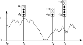
Figure 1: In this example, samples of size ${n}_{1}=4$, ${n}_{2}=3$ and ${n}_{3}=6$ (illustrated by the total number of circles) are taken at times ${t}_{1}$, ${t}_{2}$ and ${t}_{3}$, respectively. The observed number of derived alleles (filled circles) is $d_{1}=3$, $d_{2}=1$ and $d_{3}=4$. The initial time is ${t}_{0}$, and the curve indicates a particular trajectory of the underlying population allele frequency $\mathbf{Y}({t})\in[0,1]$.

2.3 Hidden Markov model framework

To analyze the time series data described earlier, we employ a hidden Markov model (HMM) framework as in Bollback, York and Nielsen (2008). In this approach, the population-wide frequency $\mathbf{Y}({\tau})$ of the $A_{1}$ allele at time ${\tau}$ is modeled as an unobserved hidden variable (see Figure 1). We denote a realization of the frequencies at the sampling times ${\tau}_{k}$ by ${y}_{k}\equiv\mathbf{Y}({\tau}_{k})$. The initial frequency at time ${\tau}_{0}$ is distributed according to the density function ${\rho}$, that is, $\mathbf{Y}({\tau}_{0})\sim{\rho}$. For example, the density function ${\rho}({y})=\delta({y}-1/(2N_{e}))$ models the case where the selected allele $A_{1}$ arose as a de novo mutation in one individual of the population at time ${\tau}_{0}$.

The probability of transitioning from frequency ${y}_{{k}-1}$ at time ${t}_{{k}-1}$ to frequency ${y}_{{k}}$ at time ${t}_{{k}}$ is described by the transition density function ${p}_{\Theta}({\tau}_{{k}}-{\tau}_{{k}-1};{y}_{{k}-1},{y}_{{k}})$ of the Wright–Fisher diffusion process, where $\Theta=({{\sigma}_{1}},{{\sigma}_{2}},{\alpha},{\beta},{\tau}_{0},N_{e})$ and ${\tau}_{k}$ are population-scaled parameters as given in equations (1)–(4). The observations in the HMM are the number of copies $d_{k}$ of the allele $A_{1}$ among the ${n}_{k}$ alleles in the sample drawn at time ${t}_{k}$. The probability of such an observation at time ${t}_{k}$ with population allele frequency ${y}_{k}$ is given by the probability mass function ${\xi}(d_{k};{n}_{k},{y}_{k})$ of a binomial distribution

$${\xi}({d}_{k};{n}_{k},{y}_{k}):=\pmatrix{{n}_{k}\cr{d}_{k}}{y}_{k}^{{d}_{k}}(1-{y}_{k})^{{n}_{k}-{d}_{k}}.$$

To compute the probability ${\mathbb{P}}_{\Theta}\{{O}_{[1\dvtx{K}]}\}$ of observing the data ${O}_{[1\dvtx{K}]}$ under the model parameters $\Theta$, we introduce the forward density functions $f_{k}$, given by

$$f_{k}({y})\,d{y}:={\mathbb{P}}_{\Theta}\bigl{\{}{O}_{[1\dvtx{k}]},\mathbf{Y}({\tau}_{k})\in d{y}\bigr{\}},\qquad{k}\in\{0,1,\ldots,{K}\}.$$ (5)

The function $f_{k}$ is the joint density of the observed data up to time ${\tau}_{k}$ and the hidden population allele frequency at time ${\tau}_{k}$. We also find it convenient to consider a second auxiliary density function, $g_{k}$, given by

$$g_{k}({y})\,d{y}:={\mathbb{P}}_{\Theta}\bigl{\{}{O}_{[1\dvtx{k}-1]},\mathbf{Y}({\tau}_{k})\in d{y}\bigr{\}},\qquad{k}\in\{1,\ldots,{K}\}.$$ (6)

This function $g_{k}$ is the joint density of the observed data up to time ${\tau}_{{k}-1}$ and the hidden frequency at ${\tau}_{k}$. The forward density function $f_{0}$ is given by the density function for the initial allele frequency as

$$f_{0}({y})={\rho}({y}).$$

Since we approximate the time evolution of the hidden population allele frequency by the Wright–Fisher diffusion, we can get a recurrence relation between the density functions $g_{k}$ and $f_{{k}-1}$ by integrating over all possible allele frequencies at ${\tau}_{{k}-1}$:

$$g_{k}({y})=\int_{0}^{1}f_{{k}-1}({x}){p}_{\Theta}({\tau}_{k}-{\tau}_{{k}-1};{x},{y})\,d{x},$$ (7)

where ${k}\in\{1,\ldots,{K}\}$. Using the binomial distribution for sampling ${d}_{k}$ derived alleles out of ${n}_{k}$ individuals at time ${\tau}_{k}$, we get another recurrence relation between the density functions $f_{k}$ and $g_{k}$ as follows:

$$f_{k}({y})=g_{k}({y}){\xi}({d}_{k};{n}_{k},{y}).$$ (8)

Finally, the probability ${\mathbb{P}}_{\Theta}\{{O}_{[1\dvtx{K}]}\}$ of observing the data is computed by integrating over all possible hidden frequencies at the last sampling time:

$${\mathbb{P}}_{\Theta}\{{O}_{[1\dvtx{K}]}\}=\int_{0}^{1}f_{K}({y})\,d{y}.$$ (9)

Note that the equations above describe a forward-in-time procedure for computing the probability of the data ${O}_{[1\dvtx{K}]}$, where the intermediate density functions have a natural interpretation.

While (7), (8) and (9) succinctly describe the sampling probability of the data ${O}_{[1\dvtx{K}]}$, no analytic solutions to the integrals in (7) and (9) are known. In the previous approaches mentioned in the Introduction, these integrals were approximated numerically by discretizing the allele frequency state space. The accuracy of these approximations depends critically on the careful choice of the discretization grid. We present an analytical solution to this problem which obviates the need for such a discretization.

2.4 Spectral representation of the transition density

The biallelicWright–Fisher diffusion with general diploid selection has the infinitesimal generator ${\mathcal{L}}$ given by

$${\mathcal{L}} = {{\mathcal{L}}_{0}}+2{x}(1-{x})\bigl{[}{{\sigma}_{1}}(1-2{x})+{{\sigma}_{2}}{x}\bigr{]}\frac{\partial}{\partial{x}},$$ (10)

where ${{\mathcal{L}}_{0}}$ is the infinitesimal generator of the diffusion process without selection, given by

$${{\mathcal{L}}_{0}} = \frac{1}{2}{x}(1-{x})\frac{\partial^{2}}{\partial{x}^{2}}+\frac{1}{2}\bigl{[}{\alpha}(1-{x})-{\beta}{x}\bigr{]}\frac{\partial}{\partial{x}}.$$ (11)

We refer the reader to Ewens (2004) for more details about the Wright–Fisher diffusion. Song and Steinrücken (2012) developed an efficient method to compute the eigenvalues and eigenfunctions of ${\mathcal{L}}$, and we utilize that method here. A brief summary of their approach is provided below.

To approximate the spectral decomposition of the operator ${\mathcal{L}}$, consider the functions

$${H}_{m}^{(\Theta)}({x}) := e^{-\bar{\sigma}({x})/2}{R}_{m}^{({\alpha},{\beta})}(x),$$ (12)

where $\bar{\sigma}({x}):=4{{\sigma}_{1}}{x}(1-{x})+2{{\sigma}_{2}}{x}^{2}$ is the mean fitness of the population and ${R}_{m}^{({\alpha},{\beta})}({x})$ are a rescaled version of the classical orthogonal Jacobi polynomials and are defined in Section B of the supplemental article [Steinrücken, Bhaskar and Song (2014)]. The $\alpha$ and $\beta$ parameters in (12) are thepopulation-scaled mutation rates given in (3) and (4). The set$\{{H}_{m}^{(\Theta)}({x})\}_{{m}\in{\mathbb{N}}_{0}}$ forms a basis for the Hilbert space ${L}^{2}([0,1],{\pi})$ of real-valued functions on $[0,1]$ that are square integrable with respect to the stationary density ${\pi}$ of the diffusion generator ${\mathcal{L}}$. Specifically,

$${\pi}({x})=e^{\bar{\sigma}({x})}{x}^{{\alpha}-1}(1-{x})^{{\beta}-1}.$$ (13)

The basis elements ${H}_{m}^{(\Theta)}({x})$ are orthogonal with respect to the inner product ${\langle\cdot,\cdot\rangle}_{{\pi}}$ defined by ${\langle f,g\rangle}_{{\pi}}=\int_{0}^{1}f(x)g(x){\pi}(x)\,dx$.

In the basis $\{{H}_{m}^{(\Theta)}({x})\}_{{m}\in{\mathbb{N}}_{0}}$, the operator ${\mathcal{L}}$ is given by the matrix

$$\mathbf{M}:=-\Biggl{(}\bolds{\Lambda}^{({\alpha},{\beta})}+\sum_{l=0}^{4}{q}^{(\Theta)}_{l}\mathbf{G}^{l}\Biggr{)},$$ (14)

where $\bolds{\Lambda}^{({\alpha},{\beta})}:=\operatorname{diag}({\lambda}^{({\alpha},{\beta})}_{0},{\lambda}^{({\alpha},{\beta})}_{1},\ldots)$ is a diagonal matrix containing the eigenvalues of the neutral diffusion generator ${{\mathcal{L}}_{0}}$, $\mathbf{G}:=({G}_{{n},{m}}^{({\alpha},{\beta})})_{{n},{m}\in{\mathbb{N}}_{0}}$ is the matrix of coefficients from the three-term recurrence relation for the Jacobi polynomials ${R}_{m}^{({\alpha},{\beta})}({x})$, and ${q}^{(\Theta)}_{l}$ are constant coefficients defined in Section C of the supplemental article [Steinrücken, Bhaskar and Song (2014)]. Explicit expressions for the entries of $\bolds{\Lambda}^{({\alpha},{\beta})}$ and $\mathbf{G}$ are provided in equations (B.3) and (B.5), respectively, in Section B of the supplemental article.

The eigenvalues ${\lambda}_{n}$ of the full diffusion generator ${\mathcal{L}}$ are given by the eigenvalues of $\mathbf{M}$, and the coefficients of the eigenfunctions of ${\mathcal{L}}$ in the basis $\{{H}_{m}^{(\Theta)}({x})\}_{{m}\in{\mathbb{N}}_{0}}$ are given by the eigenvectors of $\mathbf{M}$. In particular, the eigenfunction ${B}_{n}$ of ${\mathcal{L}}$ is given by

$${B}_{n}({x})=\sum_{{m}=0}^{\infty}{w}_{{n},{m}}{H}_{m}^{(\Theta)}({x}),$$ (15)

where $\mathbf{w}_{n}=({w}_{{n},0},{w}_{{n},1},\ldots)$ is the eigenvector of $\mathbf{M}$ corresponding to eigenvalue ${\lambda}_{n}$. We use $\bolds{\Lambda}=\operatorname{diag}({\lambda}_{0},{\lambda}_{1},\ldots)$ to denote the diagonal matrix of eigenvalues of $\mathbf{M}$, and $\mathbf{W}$ to denote the matrix with rows given by the eigenvectors $\mathbf{w}_{n}$. As can be seen from (15), $\mathbf{W}$ is the change-of-basis matrix between the basis of eigenfunctions ${B}_{n}$ of ${\mathcal{L}}$ and the basis $\{{H}_{m}^{(\Theta)}({x})\}_{{m}\in{\mathbb{N}}_{0}}$.

The leading eigenvalues and the associated eigenvectors of the infinite matrix $\mathbf{M}$ can be approximated by the eigenvalues and eigenvectors of sufficiently large submatrices of $\mathbf{M}$. We refer the reader to Song and Steinrücken (2012) for a more detailed empirical discussion on how the approximation accuracy varies for different submatrix sizes and different parameter regimes. The transition density function ${p}_{\Theta}({\tau};x,y)$ for the probability density of the allele changing frequency from $x$ to $y$ in time ${\tau}$ is given by the following spectral decomposition:

$${p}_{\Theta}({\tau};{x},{y}) = \sum_{{n}=0}^{\infty}e^{-{\lambda}_{n}{\tau}}{\pi}(y)\frac{{B}_{n}(x){B}_{n}(y)}{{\langle{B}_{n},{B}_{n}\rangle}_{{\pi}}}.$$ (16)

2.5 Incorporating the spectral representation into the HMM

Using the spectral decomposition of the transition density function in (16), we devise a dynamic programming algorithm to compute the likelihood ${\mathbb{P}}_{\Theta}\{{O}_{[1\dvtx{K}]}\}$. This algorithm recursively computes the density functions $f_{k}$ and $g_{k}$ given in (5) and (6), respectively. To update these density functions efficiently, we represent them in the basis of scaled eigenfunctions $\{{\pi}({y}){B}_{n}({y})\}_{{n}\in{\mathbb{N}}_{0}}$ of the diffusion generator ${\mathcal{L}}$. More precisely, we express $f_{k}$ and $g_{k}$ as

$$f_{k}({y}) = {\pi}({y})\mathbf{b}_{k}\mathbf{B}({y})=\sum_{{n}=0}^{\infty}{b}_{{k},{n}}{\pi}({y}){B}_{{n}}({y}),$$ (17)

$$g_{k}({y}) = {\pi}({y})\mathbf{a}_{k}\mathbf{B}({y})=\sum_{{n}=0}^{\infty}{a}_{{k},{n}}{\pi}({y}){B}_{{n}}({y}),$$ (18)

where we employ the vector notation

$$\mathbf{b}_{k} := ({b}_{{k},0},{b}_{{k},1},\ldots),$$ (19)

$$\mathbf{a}_{k} := ({a}_{{k},0},{a}_{{k},1},\ldots),$$ (20)

$$\mathbf{B}({y}) := \bigl{(}{B}_{0}({y}),{B}_{1}({y}),\ldots\bigr{)}^{T}.$$ (21)

We now describe how the coefficient vectors $\mathbf{a}_{k},\mathbf{b}_{k}$ and the probability ${\mathbb{P}}_{\Theta}\{{O}_{[1\dvtx{K}]}\}$ can be computed efficiently. All proofs can be found in Section A of the supplemental article [Steinrücken, Bhaskar and Song (2014)]. First, the following proposition determines the vector $\mathbf{b}_{0}$ of coefficients for the initial forward density function $f_{0}$:

Proposition 1

If the allele frequency at ${\tau}_{0}$ is distributed according to the density function ${\rho}({y})=\delta({y}-{x})$, then the initial forward density function $f_{0}$ in the basis $\{{\pi}({y}){B}_{n}({y})\}_{{n}\in{\mathbb{N}}_{0}}$ has the vector of coefficients

$$\mathbf{b}_{0}=\biggl{(}\frac{{B}_{0}({x})}{{c}_{0}},\frac{{B}_{1}({x})}{{c}_{1}},\ldots\biggr{)},$$

where ${B}_{n}({x})$ is given by (15), and ${c}_{n}$ are the squared norms of ${B}_{n}$ given by

$${c}_{n}={\langle{B}_{n},{B}_{n}\rangle}_{{\pi}}=\sum_{{m}=0}^{\infty}({w}_{{n},{m}})^{2}{c}_{n}^{({\alpha},{\beta})},$$ (22)

where ${c}_{n}^{({\alpha},{\beta})}$ denote the squared norms of the Jacobi polynomials given in equation (B.2) in Section B of the supplemental article [Steinrücken, Bhaskar and Song (2014)].

In the case where the selected allele $A_{1}$ arises from de novo mutation at ${t}_{0}$ in one of the individuals in the population, we set ${x}=1/(2N_{e})$ in Proposition 1. We note that our framework allows us to easily model other distributions for the frequency of the mutant allele $A_{1}$ when it became selected. For example, the initial distribution of mutation-drift balance can be used to model selection arising from standing genetic variation. Some of these initial distributions are described in Section D of the supplemental article [Steinrücken, Bhaskar and Song (2014)].

The following theorem establishes how the representations of the densities $f_{k}$ and $g_{k}$, for ${k}>0$, can be computed algebraically in a recursive fashion:

Theorem 2

Let $\mathbf{C}:=\operatorname{diag}({c}_{0}^{({\alpha},{\beta})},{c}_{1}^{({\alpha},{\beta})},\ldots)$ and $\mathbf{D}:=\operatorname{diag}({c}_{0},{c}_{1},\ldots)$ denote diagonal matrices with entries ${c}_{n}^{({\alpha},{\beta})}$ and ${c}_{n}$ defined as in Proposition 1. Then, for each ${k}\in\{1,\ldots,{K}\}$, the coefficients in the representation of the densities $g_{k}({y})$ and $f_{k}({y})$ in (17) and (18) can be computed recursively as

$$\mathbf{a}_{k} = \mathbf{b}_{{k}-1}\exp\bigl{[}-\bolds{\Lambda}({\tau}_{k}-{\tau}_{{k}-1})\bigr{]},$$ (23)

$$\mathbf{b}_{k} = \mathbf{a}_{k}\mathbf{W}\mathbf{G}^{{d}_{k}}(\mathbf{1}-\mathbf{G})^{{n}_{k}-{d}_{k}}\mathbf{W}^{-1},$$ (24)

where $\mathbf{W}^{-1}$ is given by

$$\mathbf{W}^{-1} = \mathbf{C}\mathbf{W}^{T}\mathbf{D}^{-1}.$$ (25)

Combining Proposition 1 and Theorem 2, we obtain a dynamic programming algorithm for calculating the coefficients $\mathbf{b}_{k}$ and $\mathbf{a}_{k}$ in the representations for $f_{k}$ and $g_{k}$ given in (17) and (18), respectively. The vectors and matrices appearing in the above results are infinite dimensional. As in previous works [Song and Steinrücken (2012), Steinrücken, Wang and Song (2013)] on the spectral representation of the transition density, when applying the above results we truncate the infinite vectors and matrices by choosing cutoffs for the dimensions. We provide more practical details in Section 3.3.

Finally, the probability of observing the full data ${O}_{[1\dvtx{K}]}$ can be computed using the following proposition:

Proposition 3

The probability ${\mathbb{P}}_{\Theta}\{{O}_{[1\dvtx{K}]}\}$ of observing the data ${O}_{[1\dvtx{K}]}$ given the population genetic parameters $\Theta$ is

$${\mathbb{P}}_{\Theta}\{{O}_{[1\dvtx{K}]}\}=\frac{{c}_{0}}{{B}_{0}(0)}{b}_{{K},0},$$ (26)

where ${B}_{0}(0)$ is given by

$${B}_{0}(0)=\sum_{{m}=0}^{\infty}(-1)^{m}{w}_{0,{m}}\frac{\Gamma({m}+{\alpha})}{\Gamma({m}+1)\Gamma({\alpha})}.$$

3 Results

In this section we perform parametric inference via the maximum likelihood framework using a finite grid in the parameter space. We first test the accuracy on simulated data and then apply it to analyze an ancient DNA data set related to coat coloration in domesticated horses [Ludwig et al. (2009)].

Since ancient DNA data are often collected from only those loci which are segregating at the present time, in our empirical study we condition on observing at least one copy of the derived allele at the last sampling time ${\tau}_{K}$. In particular, the likelihood of the parameters is given by $L(\Theta):={\mathbb{P}}_{\Theta}\{{O}_{[1\dvtx{K}]}|{d}_{K}>0\}$. We chose to maximize this function on a grid, since the algorithm described in the previous section can be parallelized, thus allowing to efficiently evaluate the likelihood under given parameters for several data sets at once.

3.1 Performance on simulated data

We simulated data under a discrete-time Wright–Fisher model with several values for the effective population size and selection coefficients. We chose the mutation probabilities to be ${u_{01}}={u_{10}}=10^{-6}$ and the number of years per generation to be five years. These parameters are similar to those considered by previous works that analyzed time series allelic samples from the ASIP and MC1R loci in horses [Ludwig et al. (2009), Malaspinas et al. (2012)]. In our simulations, 5% of the population carried the mutant allele when it first became positively selected. We sampled 40 individuals at each of 10 time points over the course of 32,000 years.

We investigated the performance of our maximum likelihood estimator in various scenarios of selection. Here, we present the results for the following four particular selection schemes: [2.]

Genic selection, in which the selective fitness of the heterozygote is the arithmetic mean of the fitness of the two homozygotes, that is, ${{s}_{1}}={s}/2$ and ${{s}_{2}}={s}$.

Heterozygote advantage selection, in which ${{s}_{1}}={s}$ and ${{s}_{2}}=0$.

Recessive selection, in which ${{s}_{1}}=0$, ${{s}_{2}}={s}$.

Dominant selection, in which ${{s}_{1}}={s}$, ${{s}_{2}}={s}$. For each scenario, we considered ${s}\in\{0,0.001,0.0025,0.005,0.01\}$ and simulated 200 data sets for each value of $s$.

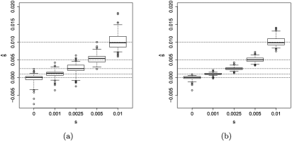
Figure 2: Empirical distribution of the maximum likelihood estimates for 200 data sets simulated under a model of genic selection, with heterozygote fitness ${{s}_{1}}={s}/2$ and derived allele homozygote fitness ${{s}_{2}}={s}$, for each of several different values of selection strength ${s}$. The dashed lines indicate the true values. (a) The effective population size $N_{e}$ is 2500 individuals. (b) $N_{e}={}$10,000 individuals.

Figure 2 shows the performance of the maximum likelihood estimator under a model of genic selection with an effective population size of $N_{e}=2500$ and $N_{e}={}$10,000. It illustrates empirical boxplots of the maximum likelihood estimates, where the tips of the whiskers denote the 2.5%-quantile and the 97.5%-quantile, and the boxes represent the upper and lower quartile. As the figure shows, our maximum likelihood estimates are unbiased. The uncertainty of the estimate tends to increase with increasing values of ${s}$, while the uncertainty decreases as the population size increases, illustrating the fact that for larger population sizes, selection acts more efficiently and is easier to detect. In the case of $N_{e}={}$10,000, if the true selection coefficient is $0.0025$ or more, all our maximum likelihood estimates are higher than the 97.5%-quantile of the empirical distribution of the maximum likelihood estimates for ${s}=0$. Hence, there is high power to reject neutrality in these scenarios.

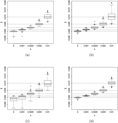
Figure 3: Empirical distribution of the maximum likelihood estimates of 200 simulated data sets each under different modes of selection of differing strength with $N_{e}={}$10,000. The dashed lines indicate the true values of ${s}$. (a) Genic selection (${{s}_{1}}={s}/2$, ${{s}_{2}}={s}$) with only five sampling time points. (b) Heterozygote advantage model of selection (${{s}_{1}}={s}$, ${{s}_{2}}=0$) with ten sampling time points. (c) Recessive selection (${{s}_{1}}=0$, ${{s}_{2}}={s}$) with ten sampling time points. (d) Dominant selection (${{s}_{1}}={s}$, ${{s}_{2}}={s}$) with ten sampling time points.

The performance of our maximum likelihood estimator for several additional selection schemes and parameter regimes can be found in Figure 3, where we also consider a scenario with fewer sampling time points. The figure shows that our maximum likelihood estimates are unbiased across the different parameter ranges and scenarios. In general, the low variance of the empirical distribution of the maximum likelihood estimates shows that our method can be used to accurately infer the selection parameters of interest in a wide range of scenarios.

3.2 Analysis of ancient DNA data: Coat coloration in domesticated horses

Ludwig et al. (2009) extracted genotype data at several loci from ancient horse DNA obtained from various sites in Eurasia. In particular, they extracted temporal allele frequency data at eight loci that are known to play a role in coat color determination in contemporary horses. Only the locus encoding for the Agouti signaling peptide (ASIP) and the locus for the melanocortin 1 receptor (MC1R) showed strong fluctuations in the sample allele counts. Table 1 shows the time series data for the ASIP and the MC1R loci in the curated form of the original work [Ludwig et al. (2009)].

Using the method of Bollback, York and Nielsen (2008) for the model of genic selection (${{s}_{1}}={s}/2$, ${{s}_{2}}={s}$), Ludwig et al. (2009) established that selection acted significantly on only the ASIP and the MC1R loci. However, another recent analysis [Malaspinas et al. (2012)] of the same data set considered the model of recessive selection (${{s}_{1}}=0$, ${{s}_{2}}={s}$) and did not find a significant signal of selection at the ASIP locus.

Table 1: The temporal allele frequency data sets for the ASIP and MC1R loci associated with coat coloration in domesticated horses [Ludwig et al. (2009), Figure S.3]. For each sampling time ${t}_{{k}}$ (given in years BCE), the table lists the number ${d}_{{k}}$ of derived alleles among the sampled ${n}_{{k}}$ alleles

Time of sampling [${t}_{k}$] (BCE)	$20{,}000$	$13{,}100$	$3700$	$2800$	$1100$	$500$
# of samples [${n}_{k}$]	$10$	$22$	$20$	$20$	$36$	$38$
ASIP (# der. alleles) [${d}_{k}$]	$0$	$1$	$15$	$12$	$15$	$18$
MC1R (# der. alleles) [${d}_{k}$]	$0$	$0$	$1$	$6$	$13$	$24$

To investigate the dependence of the previous conclusions on the assumed selection scheme, we applied our method to reanalyze the ASIP and the MC1R data under a general selection scheme with arbitrary selection coefficients ${{s}_{1}}$ and ${{s}_{2}}$. We set the mutation probability to ${u_{01}}={u_{10}}=10^{-6}$ and the average length of a generation to 5 years. Table 1 shows that the derived allele is absent in both data sets at time 20,000 BCE. Thus, we set the initial frequency of the derived allele as $1/2N_{e}$, corresponding to the case where the selected allele arises as a de novo mutation at time ${t}_{0}$. We tried a range of values for $N_{e}$ and ${t}_{0}$.

Figure 4(a) shows the likelihood surface for the temporal allele frequency data from the ASIP locus, for $N_{e}=2500$ and ${t}_{0}={}$17,000 BCE. The empirical maximum of the likelihood surface is located at $({{s}_{1}},{{s}_{2}})=(0.0025,0)$, indicated by the “x” in Figure 4(a). This maximum suggests that a selective scheme of heterozygote advantage best explains the data, where both the ancestral and derived allele homozygotes are of equal fitness, while the heterozygous genotype confers a selective advantage over the homozygotes. To establish the significance of this finding, we performed the following bootstrap procedure: we resampled the ASIP data set 100 times to obtain subsampled data sets $\{{O}_{[1\dvtx{K}]}^{({j})}\}_{{j}=1}^{100}$. For each bootstrapped data set $1\leq{j}\leq 100$, we resampled ${n}_{k}^{({j})}={n}_{k}$ alleles at each time ${t}_{k}^{({j})}={t}_{k}$. The number of derived alleles for data set ${j}$ was obtained by binomial sampling from the empirical frequency of derived alleles in the original ASIP data set, that is,

$${d}_{k}^{({j})}\sim{\xi}\biggl{(}\cdot;{n}_{k}^{({j})},\frac{{d}_{k}}{{n}_{k}}\biggr{)}.$$

We then reported the empirical maximum of the likelihood surface for each of these resampled data sets. Figure 4(b) shows the empirical maximum likelihood estimates and marginal histograms of the maxima for the 100 resampled data sets. The marginal 2.5% and 97.5% quantiles of the empirical distribution are $[0.0025,0.0235]$ for the heterozygote fitness ${{s}_{1}}$ and $[0,0.0045]$ for the derived allele homozygote fitness ${{s}_{2}}$, thus providing further evidence that the data are significantly better explained by a selection model where a heterozygous individual is selectively advantageous over the homozygous individuals. As Figure 5 shows, changing $N_{e}$ from 1000 to 10,000, or changing ${t}_{0}$ from 19,000 BCE to 15,000, BCE has only a minimal effect on the shape of the likelihood surface and maximum likelihood estimate, again supporting that a selective scheme of heterozygote advantage best explains the data.

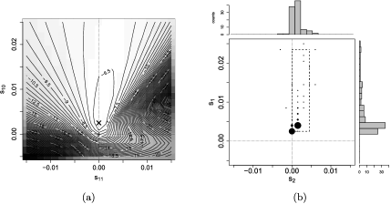
Figure 4: Analysis of the ASIP locus. (a) Empirical values of the likelihood $L(\Theta)$ for temporal samples from the ASIP locus where the likelihood is computed over a $21\times 21$ grid. The maximum is attained at $({{s}_{1}},{{s}_{2}})=(0.0025,0)$, indicated by the “x.” (b) A joint density plot and marginal histograms of the maximum likelihood estimates for 100 bootstrap resampled data sets of the temporal data at the ASIP locus. The circles are centered on the grid points at which the likelihood function is evaluated, and the sizes of the circles indicate the proportion of maximum likelihood estimates that occupy the same grid point. The marginal empirical 2.5% and 97.5%-quantiles are $[0.0025,0.0235]$ for the heterozygote fitness ${{s}_{1}}$, and $[0,0.0045]$ for the derived allele homozygote fitness ${{s}_{2}}$, as indicated by the dashed box.

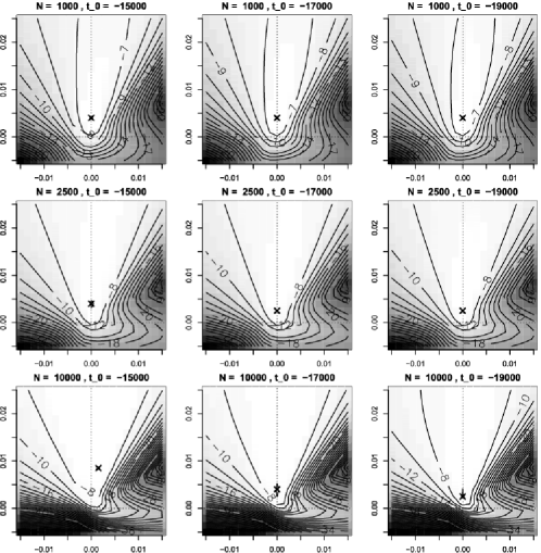
Figure 5: Likelihood surfaces for the ASIP data set under various combinations of $N_{e}\in{}${1000, 2500, 10,000} and ${t}_{0}\in{}${15,000 BCE, 17,000 BCE, 19,000 BCE}. The respective maxima are indicated by an “x.”

A similar analysis of the MC1R locus can be found in Figures 6 and 7. For this data set, the maximum of the likelihood surface is attained at $({{s}_{1}},{{s}_{2}})=(0.004,0.0015)$, and the empirical marginal 2.5% and 97.5%-quantiles are $[0.001,0.025]$ for the heterozygote fitness and $[-0.009,0.0135]$ for the derived allele homozygote fitness. Together with the results shown in Figure 7, this suggests that the data at the MC1R locus is also best explained by a selection model of heterozygote advantage. However, although the marginal quantiles for the homozygote fitness cover ${{s}_{2}}=0$, they are rather far apart, so the evidence of heterozygote advantage for the MC1R locus is weaker than that for the ASIP locus.

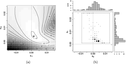
Figure 6: Analysis of the MC1R locus using the parameters $N_{e}=2500$ and ${t}_{0}=7000$ BCE. (a) Likelihood surface for the MC1R locus. The maximum likelihood estimate is at $({{s}_{1}},{{s}_{2}})=(0.004,0.0015)$ and is indicated by the “x.” (b) A joint density plot and marginal histograms of the maximum likelihood estimates for 100 bootstrap resampled data sets obtained from the MC1R data as described in Section 3.2. The marginal 2.5% and 97.5%-quantiles are $[0.001,0.025]$ for the heterozygote fitness $s_{1}$ and $[-0.009,0.0135]$ for the derived allele homozygote fitness $s_{2}$, as indicated by the dashed box.

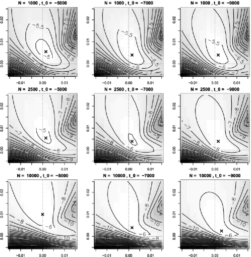
Figure 7: Likelihood surfaces for the MC1R data set under various combinations of $N_{e}\in{}${1000, 2500, 10,000} and ${t}_{0}\in{}${5000 BCE, 7000 BCE, 9000 BCE}. The respective maxima are indicated by an “x.”

3.3 Computational performance

The running time of our algorithm for computing the likelihood of a given set of population-scaled parameters is dependent on the dimensions of the truncation $\widetilde{\mathbf{M}}$ of the infinite matrix $\mathbf{M}$ given in (14). In particular, the time complexity of computing a single likelihood is the cost of computing the eigenvalues and eigenvectors of $\widetilde{\mathbf{M}}$ plus the cost of computing the coefficients $\mathbf{b}_{k}$ in Theorem 2, where $k\in\{1,\ldots,K\}$. To compute the eigenvalues and eigenvectors of $\widetilde{\mathbf{M}}$ to high precision, we first used LAPACK to compute them to double precision, and then refine them by using inverse iteration [Press et al. (2007), Chapter 11.8]. Each step of the inverse iteration involves solving a linear system with matrix $\widetilde{\mathbf{M}}-\mu\mathbf{I}$, where $\mu$ is an estimate for an eigenvalue of $\widetilde{\mathbf{M}}$. Since this matrix has bandwidth at most 9, this linear system can be solved in $O(D)$ time, where $D$ is the dimension of $\widetilde{\mathbf{M}}$. By using the repeated squaring algorithm for taking powers of the matrices $\mathbf{G}$ and $\mathbf{1}-\mathbf{G}$ and exploiting the fact that $\mathbf{G}$ and $\mathbf{1}-\mathbf{G}$ are tridiagonal matrices, each coefficient $\mathbf{b}_{k}$ can be computed in $O(D^{2}+D\min(D,n_{k})^{2}\log n_{k})$ time, where the first $O(D^{2})$ term comes from the matrix-vector multiplications in (24).

For the analysis of the ASIP and MC1R data sets reported in Figures 4 and 6, we approximated the eigenvalues and eigenvectors of $\mathbf{M}$ defined in (14) using a $600\times 600$ submatrix. Furthermore, we used the first $590$ terms in (15) to approximate the eigenfunctions, and the dimensions of the vectors of coefficients in (19) and (20) were set to $580$. We empirically verified that these cutoffs produced a stable approximation of the likelihood. Using these values, the computation time for a single point of the grid in Figure 4(a) was approximately 95 seconds. We adjusted the cutoffs appropriately for the other analyses reported in Section 3.

4 Discussion

In this paper we have developed a novel, efficient spectral algorithm to analyze time series allele frequency data under a general diploid selection model. We have demonstrated that our method can be used to accurately estimate selection parameters on simulated data.

We have also applied our method to investigate loci involved in horse coat coloration. Our inferred selection coefficients show that the data are best explained by a heterozygote advantage model of balancing selection. As mentioned earlier, Ludwig et al. (2009) provided evidence for slightly positive selection at the ASIP locus, assuming a model of genic selection (where ${{s}_{1}}={{s}_{2}}/2$). More precisely, they obtained a point estimate of ${{s}_{2}}=0.0007$ and a 95% confidence interval of $[0.0001,0.0015]$. However, using a model of selection where the derived allele homozygote is recessive (i.e., ${{s}_{1}}=0$), a subsequent reanalysis [Malaspinas et al. (2012)] of the same data found that ${{s}_{2}}$ has a point estimate of $-$0.001 with a 95% confidence interval of $[-0.02,0.051]$, thus not rejecting neutrality at the ASIP locus. In our work, we have allowed our method to explore the two-dimensional parameter space of general diploid selection models and presented evidence for a selection mode where heterozygous individuals are advantageous over homozygous individuals. It is possible that previous analyses have only been able to infer very weak selection acting at the ASIP locus because they have restricted the model of selection to certain one-dimensional models. Indeed, if we restrict our analysis to a model of genic selection, we get results similar to those reported by Ludwig et al. (2009). Our analysis does not conclusively prove that individuals that were heterozygous at the ASIP locus had a constant evolutionary advantage since 17,000 BCE, because we have ignored the interaction of selection and demographic history, epistatic interactions between loci, time-varying models of selection and other factors. However, our results suggest the possibility that some mode of heterozygote advantage balancing selection has maintained polymorphism at the ASIP locus that is involved in horse coat coloration.

Although we have focused on time series samples taken at a biallelic locus, the mathematical framework presented here could be readily extended to handle an arbitrary number of alleles using the spectral representation derived by Steinrücken, Wang and Song (2013). Further, changes in the population size and selection coefficients could be modeled by suitably combining the spectral representations for different population genetic parameters at the change points. It is also possible to extend the method to multiple populations and to incorporate samples taken from extinct ancestral populations. In light of emerging ancient DNA sequence data for ancient hominids [Green et al. (2010), Reich et al. (2010)], such temporal sequence data and inference methods present novel opportunities to gain insight into adaptation in humans. For a more adequate modeling of biologically relevant scenarios, it is also necessary to incorporate the exchange of migrants into the model [Gutenkunst et al. (2009), Lukić, Hey and Chen (2011)] and extend the framework to incorporate variation at linked loci. By taking advantage of genetic hitchhiking at closely linked sites during the course of selective sweeps, one might be able to further improve the inference of selection coefficients.

References

- Bollback, York and Nielsen (2008) {barticle}[author] \bauthor\bsnmBollback, \bfnmJonathan P.\binitsJ. P., \bauthor\bsnmYork, \bfnmThomas L.\binitsT. L. and \bauthor\bsnmNielsen, \bfnmRasmus\binitsR. (\byear2008). \btitleEstimation of from temporal allele frequency data. \bjournalGenetics \bvolume179 \bpages497–502. \bptokimsref\endbibitem
- Burke et al. (2010) {barticle}[pbm] \bauthor\bsnmBurke, \bfnmMolly K.\binitsM. K., \bauthor\bsnmDunham, \bfnmJoseph P.\binitsJ. P., \bauthor\bsnmShahrestani, \bfnmParvin\binitsP., \bauthor\bsnmThornton, \bfnmKevin R.\binitsK. R., \bauthor\bsnmRose, \bfnmMichael R.\binitsM. R. and \bauthor\bsnmLong, \bfnmAnthony D.\binitsA. D. (\byear2010). \btitleGenome-wide analysis of a long-term evolution experiment with Drosophila. \bjournalNature \bvolume467 \bpages587–590. \biddoi=10.1038/nature09352, issn=1476-4687, pii=nature09352, pmid=20844486 \bptokimsref\endbibitem
- Ewens (2004) {bbook}[mr] \bauthor\bsnmEwens, \bfnmWarren J.\binitsW. J. (\byear2004). \btitleMathematical Population Genetics: I. Theoretical Introduction, \bedition2nd ed. \bpublisherSpringer, \blocationNew York. \biddoi=10.1007/978-0-387-21822-9, mr=2026891 \bptokimsref\endbibitem
- Fearnhead (2003) {barticle}[pbm] \bauthor\bsnmFearnhead, \bfnmPaul\binitsP. (\byear2003). \btitleAncestral processes for non-neutral models of complex diseases. \bjournalTheor. Popul. Biol. \bvolume63 \bpages115–130. \bidissn=0040-5809, pii=S0040580902000497, pmid=12615495 \bptokimsref\endbibitem
- Fearnhead (2006) {barticle}[pbm] \bauthor\bsnmFearnhead, \bfnmPaul\binitsP. (\byear2006). \btitleThe stationary distribution of allele frequencies when selection acts at unlinked loci. \bjournalTheor. Popul. Biol. \bvolume70 \bpages376–386. \biddoi=10.1016/j.tpb.2006.02.001, issn=0040-5809, pii=S0040-5809(06)00015-3, pmid=16563450 \bptokimsref\endbibitem
- Feder, Kryazhimskiy and Plotkin (2014) {barticle}[pbm] \bauthor\bsnmFeder, \bfnmAlison F.\binitsA. F., \bauthor\bsnmKryazhimskiy, \bfnmSergey\binitsS. and \bauthor\bsnmPlotkin, \bfnmJoshua B.\binitsJ. B. (\byear2014). \btitleIdentifying signatures of selection in genetic time series. \bjournalGenetics \bvolume196 \bpages509–522. \biddoi=10.1534/genetics.113.158220, issn=1943-2631, pii=genetics.113.158220, pmcid=3914623, pmid=24318534 \bptokimsref\endbibitem
- Genz and Joyce (2003) {barticle}[author] \bauthor\bsnmGenz, \bfnmAlan\binitsA. and \bauthor\bsnmJoyce, \bfnmPaul\binitsP. (\byear2003). \btitleComputation of the normalizing constant for exponentially weighted Dirichlet distribution integrals. \bjournalComputing Science and Statistics \bvolume35 \bpages181–212. \bptokimsref\endbibitem
- Green et al. (2010) {barticle}[author] \bauthor\bsnmGreen, \bfnmRichard E.\binitsR. E., \bauthor\bsnmKrause, \bfnmJohannes\binitsJ., \bauthor\bsnmBriggs, \bfnmAdrian W.\binitsA. W., \bauthor\bsnmMaricic, \bfnmTomislav\binitsT., \bauthor\bsnmStenzel, \bfnmUdo\binitsU., \bauthor\bsnmKircher, \bfnmMartin\binitsM., \bauthor\bsnmPatterson, \bfnmNick\binitsN., \bauthor\bsnmLi, \bfnmHeng\binitsH., \bauthor\bsnmZhai, \bfnmWeiwei\binitsW., \bauthor\bsnmFritz, \bfnmMarkus Hsi-Yang\binitsM. H.-Y. \betalet al. (\byear2010). \btitleA draft sequence of the Neandertal genome. \bjournalScience \bvolume328 \bpages710–722. \bptokimsref\endbibitem
- Gutenkunst et al. (2009) {barticle}[pbm] \bauthor\bsnmGutenkunst, \bfnmRyan N.\binitsR. N., \bauthor\bsnmHernandez, \bfnmRyan D.\binitsR. D., \bauthor\bsnmWilliamson, \bfnmScott H.\binitsS. H. and \bauthor\bsnmBustamante, \bfnmCarlos D.\binitsC. D. (\byear2009). \btitleInferring the joint demographic history of multiple populations from multidimensional SNP frequency data. \bjournalPLoS Genet. \bvolume5 \bpagese1000695. \biddoi=10.1371/journal.pgen.1000695, issn=1553-7404, pmcid=2760211, pmid=19851460 \bptokimsref\endbibitem
- Hummel et al. (2005) {barticle}[pbm] \bauthor\bsnmHummel, \bfnmS.\binitsS., \bauthor\bsnmSchmidt, \bfnmD.\binitsD., \bauthor\bsnmKremeyer, \bfnmB.\binitsB., \bauthor\bsnmHerrmann, \bfnmB.\binitsB. and \bauthor\bsnmOppermann, \bfnmM.\binitsM. (\byear2005). \btitleDetection of the CCR5-Delta32 HIV resistance gene in Bronze Age skeletons. \bjournalGenes Immun. \bvolume6 \bpages371–374. \biddoi=10.1038/sj.gene.6364172, issn=1466-4879, pii=6364172, pmid=15815693 \bptokimsref\endbibitem
- Lang et al. (2013) {barticle}[pbm] \bauthor\bsnmLang, \bfnmGregory I.\binitsG. I., \bauthor\bsnmRice, \bfnmDaniel P.\binitsD. P., \bauthor\bsnmHickman, \bfnmMark J.\binitsM. J., \bauthor\bsnmSodergren, \bfnmErica\binitsE., \bauthor\bsnmWeinstock, \bfnmGeorge M.\binitsG. M., \bauthor\bsnmBotstein, \bfnmDavid\binitsD. and \bauthor\bsnmDesai, \bfnmMichael M.\binitsM. M. (\byear2013). \btitlePervasive genetic hitchhiking and clonal interference in forty evolving yeast populations. \bjournalNature \bvolume500 \bpages571–574. \biddoi=10.1038/nature12344, issn=1476-4687, mid=NIHMS488396, pii=nature12344, pmcid=3758440, pmid=23873039 \bptokimsref\endbibitem
- Ludwig et al. (2009) {barticle}[pbm] \bauthor\bsnmLudwig, \bfnmArne\binitsA., \bauthor\bsnmPruvost, \bfnmMelanie\binitsM., \bauthor\bsnmReissmann, \bfnmMonika\binitsM., \bauthor\bsnmBenecke, \bfnmNorbert\binitsN., \bauthor\bsnmBrockmann, \bfnmGudrun A.\binitsG. A., \bauthor\bsnmCastaños, \bfnmPedro\binitsP., \bauthor\bsnmCieslak, \bfnmMichael\binitsM., \bauthor\bsnmLippold, \bfnmSebastian\binitsS., \bauthor\bsnmLlorente, \bfnmLaura\binitsL., \bauthor\bsnmMalaspinas, \bfnmAnna-Sapfo\binitsA.-S., \bauthor\bsnmSlatkin, \bfnmMontgomery\binitsM. and \bauthor\bsnmHofreiter, \bfnmMichael\binitsM. (\byear2009). \btitleCoat color variation at the beginning of horse domestication. \bjournalScience \bvolume324 \bpages485. \biddoi=10.1126/science.1172750, issn=1095-9203, pii=324/5926/485, pmid=19390039 \bptokimsref\endbibitem
- Lukić, Hey and Chen (2011) {barticle}[pbm] \bauthor\bsnmLukić, \bfnmSergio\binitsS., \bauthor\bsnmHey, \bfnmJody\binitsJ. and \bauthor\bsnmChen, \bfnmKevin\binitsK. (\byear2011). \btitleNon-equilibrium allele frequency spectra via spectral methods. \bjournalTheor. Popul. Biol. \bvolume79 \bpages203–219. \biddoi=10.1016/j.tpb.2011.02.003, issn=1096-0325, mid=NIHMS284088, pii=S0040-5809(11)00016-5, pmcid=3410934, pmid=21376069 \bptokimsref\endbibitem
- Malaspinas et al. (2012) {barticle}[author] \bauthor\bsnmMalaspinas, \bfnmA. S.\binitsA. S., \bauthor\bsnmMalaspinas, \bfnmO.\binitsO., \bauthor\bsnmEvans, \bfnmS. N.\binitsS. N. and \bauthor\bsnmSlatkin, \bfnmM.\binitsM. (\byear2012). \btitleEstimating allele age and selection coefficient from time-serial data. \bjournalGenetics \bvolume192 \bpages599–607. \bptokimsref\endbibitem
- Mathar (2009) {barticle}[author] \bauthor\bsnmMathar, \bfnmR. J.\binitsR. J. (\byear2009). \btitleA Java Math.BigDecimal implementation of core mathematical functions. \bnoteAvailable at \arxivurlarXiv:0908.3030. \bptokimsref\endbibitem
- Mathieson and McVean (2013) {barticle}[pbm] \bauthor\bsnmMathieson, \bfnmIain\binitsI. and \bauthor\bsnmMcVean, \bfnmGil\binitsG. (\byear2013). \btitleEstimating selection coefficients in spatially structured populations from time series data of allele frequencies. \bjournalGenetics \bvolume193 \bpages973–984. \biddoi=10.1534/genetics.112.147611, issn=1943-2631, pii=genetics.112.147611, pmcid=3584010, pmid=23307902 \bptokimsref\endbibitem
- Orlando et al. (2013) {barticle}[author] \bauthor\bsnmOrlando, \bfnmLudovic\binitsL., \bauthor\bsnmGinolhac, \bfnmAurélien\binitsA., \bauthor\bsnmZhang, \bfnmGuojie\binitsG., \bauthor\bsnmFroese, \bfnmDuane\binitsD., \bauthor\bsnmAlbrechtsen, \bfnmAnders\binitsA., \bauthor\bsnmStiller, \bfnmMathias\binitsM., \bauthor\bsnmSchubert, \bfnmMikkel\binitsM., \bauthor\bsnmCappellini, \bfnmEnrico\binitsE., \bauthor\bsnmPetersen, \bfnmBent\binitsB., \bauthor\bsnmMoltke, \bfnmIda\binitsI. \betalet al. (\byear2013). \btitleRecalibrating Equus evolution using the genome sequence of an early Middle Pleistocene horse. \bjournalNature \bvolume499 \bpages74–78. \bptokimsref\endbibitem
- Orozco-terWengel et al. (2012) {barticle}[pbm] \bauthor\bsnmOrozco-terWengel, \bfnmPablo\binitsP., \bauthor\bsnmKapun, \bfnmMartin\binitsM., \bauthor\bsnmNolte, \bfnmViola\binitsV., \bauthor\bsnmKofler, \bfnmRobert\binitsR., \bauthor\bsnmFlatt, \bfnmThomas\binitsT. and \bauthor\bsnmSchlötterer, \bfnmChristian\binitsC. (\byear2012). \btitleAdaptation of Drosophila to a novel laboratory environment reveals temporally heterogeneous trajectories of selected alleles. \bjournalMol. Ecol. \bvolume21 \bpages4931–4941. \biddoi=10.1111/j.1365-294X.2012.05673.x, issn=1365-294X, pmcid=3533796, pmid=22726122 \bptokimsref\endbibitem
- Press et al. (2007) {bbook}[mr] \bauthor\bsnmPress, \bfnmWilliam H.\binitsW. H., \bauthor\bsnmTeukolsky, \bfnmSaul A.\binitsS. A., \bauthor\bsnmVetterling, \bfnmWilliam T.\binitsW. T. and \bauthor\bsnmFlannery, \bfnmBrian P.\binitsB. P. (\byear2007). \btitleNumerical Recipes: The Art of Scientific Computing, \bedition3rd ed. \bpublisherCambridge Univ. Press, \blocationCambridge. \bidmr=2371990 \bptokimsref\endbibitem
- Reich et al. (2010) {barticle}[pbm] \bauthor\bsnmReich, \bfnmDavid\binitsD., \bauthor\bsnmGreen, \bfnmRichard E.\binitsR. E., \bauthor\bsnmKircher, \bfnmMartin\binitsM., \bauthor\bsnmKrause, \bfnmJohannes\binitsJ., \bauthor\bsnmPatterson, \bfnmNick\binitsN., \bauthor\bsnmDurand, \bfnmEric Y.\binitsE. Y., \bauthor\bsnmViola, \bfnmBence\binitsB., \bauthor\bsnmBriggs, \bfnmAdrian W.\binitsA. W., \bauthor\bsnmStenzel, \bfnmUdo\binitsU., \bauthor\bsnmJohnson, \bfnmPhilip L. F.\binitsP. L. F. \betalet al. (\byear2010). \btitleGenetic history of an archaic hominin group from Denisova Cave in Siberia. \bjournalNature \bvolume468 \bpages1053–1060. \biddoi=10.1038/nature09710, issn=1476-4687, pii=nature09710, pmid=21179161 \bptokimsref\endbibitem
- Shankarappa et al. (1999) {barticle}[author] \bauthor\bsnmShankarappa, \bfnmR.\binitsR., \bauthor\bsnmMargolick, \bfnmJ. B.\binitsJ. B., \bauthor\bsnmGange, \bfnmS. J.\binitsS. J., \bauthor\bsnmRodrigo, \bfnmA. G.\binitsA. G., \bauthor\bsnmUpchurch, \bfnmD.\binitsD., \bauthor\bsnmFarzadegan, \bfnmH.\binitsH., \bauthor\bsnmGupta, \bfnmP.\binitsP., \bauthor\bsnmRinaldo, \bfnmC. R.\binitsC. R., \bauthor\bsnmLearn, \bfnmG. H.\binitsG. H., \bauthor\bsnmHe, \bfnmX.\binitsX., \bauthor\bsnmHuang, \bfnmX. L.\binitsX. L. and \bauthor\bsnmMullins, \bfnmJ. I.\binitsJ. I. (\byear1999). \btitleConsistent viral evolutionary changes associated with the progression of human immunodeficiency virus type 1 infection. \bjournalJ. Virol. \bvolume73 \bpages10489–10502. \bptokimsref\endbibitem
- Song and Steinrücken (2012) {barticle}[pbm] \bauthor\bsnmSong, \bfnmYun S.\binitsY. S. and \bauthor\bsnmSteinrücken, \bfnmMatthias\binitsM. (\byear2012). \btitleA simple method for finding explicit analytic transition densities of diffusion processes with general diploid selection. \bjournalGenetics \bvolume190 \bpages1117–1129. \biddoi=10.1534/genetics.111.136929, issn=1943-2631, pii=genetics.111.136929, pmcid=3296246, pmid=22209899 \bptokimsref\endbibitem
- Steinrücken, Bhaskar and Song (2014) {bmisc}[author] \bauthor\bsnmSteinrücken, \binitsM., \bauthor\bsnmBhaskar, \binitsA. and \bauthor\bsnmSong, \binitsY. (\byear2014). \bhowpublishedSupplement to “A novel spectral method for inferring general diploid selection from time series genetic data.” DOI:\doiurl10.1214/14-AOAS764SUPP. \bptokimsref \endbibitem
- Steinrücken, Wang and Song (2013) {barticle}[author] \bauthor\bsnmSteinrücken, \bfnmMatthias\binitsM., \bauthor\bsnmWang, \bfnmY. X. R.\binitsY. X. R. and \bauthor\bsnmSong, \bfnmYun S.\binitsY. S. (\byear2013). \btitleAn explicit transition density expansion for a multi-allelic Wright–Fisher diffusion with general diploid selection. \bjournalTheor. Popul. Biol. \bvolume83 \bpages1–14. \bptokimsref\endbibitem
- Stephens and Donnelly (2003) {barticle}[mr] \bauthor\bsnmStephens, \bfnmMatthew\binitsM. and \bauthor\bsnmDonnelly, \bfnmPeter\binitsP. (\byear2003). \btitleAncestral inference in population genetics models with selection (with discussion). \bjournalAust. N. Z. J. Stat. \bvolume45 \bpages395–430. \biddoi=10.1111/1467-842X.00295, issn=1369-1473, mr=2018460 \bptnotecheck related \bptokimsref\endbibitem
- Williamson and Slatkin (1999) {barticle}[author] \bauthor\bsnmWilliamson, \bfnmEllen G.\binitsE. G. and \bauthor\bsnmSlatkin, \bfnmMongomery\binitsM. (\byear1999). \btitleUsing maximum likelihood to estimate population size from temporal changes in allele frequencies. \bjournalGenetics \bvolume152 \bpages755–761. \bptokimsref\endbibitem
- Wiser, Ribeck and Lenski (2013) {barticle}[pbm] \bauthor\bsnmWiser, \bfnmMichael J.\binitsM. J., \bauthor\bsnmRibeck, \bfnmNoah\binitsN. and \bauthor\bsnmLenski, \bfnmRichard E.\binitsR. E. (\byear2013). \btitleLong-term dynamics of adaptation in asexual populations. \bjournalScience \bvolume342 \bpages1364–1367. \biddoi=10.1126/science.1243357, issn=1095-9203, pii=science.1243357, pmid=24231808 \bptokimsref\endbibitem