Cosmology of Holographic and New Agegraphic $f(R,T)$ Models

Abstract

We consider the $f(R,T)$ theory, where $R$ is the scalar curvature and $T$ is the trace of energy-momentum tensor, as an effective description for the holographic and new agegraphic dark energy and reconstruct the corresponding $f(R,T)$ functions. In this study, we concentrate on two particular models of $f(R,T)$ gravity namely, $R+2A(T)$ and $B(R)+\lambda{T}$. We conclude that the derived $f(R,T)$ models can represent phantom or quintessence regimes of the universe which are compatible with the current observational data. In addition, the conditions to preserve the generalized second law of thermodynamics are established.

Keywords: Modified Gravity; Dark Energy; Thermodynamics.
PACS: 04.50.Kd; 95.36.+x; 97.60.Lf.

1 Introduction

Supernovae type Ia (SNeIa)¹⁾ observations revealed the expanding behavior of the universe. This fact has further been affirmed by the observations of anisotropies in cosmic microwave background (CMB)²⁾, large scale structure³⁾, baryon acoustic oscillations⁴⁾ and weak lensing⁵⁾. A strange type of energy component with prominent negative pressure identified as dark energy (DE) is used to explain the current cosmic acceleration. The source and characteristics of DE are still a complicated story as several models have been suggested in the context of general relativity (GR) (for review see⁶⁾).

The most likely campaigner of DE is the cosmological constant or the vacuum energy whose equation of state (EoS) parameter is fixed, $\omega_{\Lambda}=-1$. The cosmological model that consists of cosmological constant plus cold dark matter is entitled as ${\Lambda}CDM$ model, which appears to fit the observational data. However, despite of its success, this model experiences two notable cosmological problems namely, the “fine tuning” problem and the “cosmic coincidence” problem⁷⁾. Such issue primarily originates because the vacuum energy is counted in the setting of quantum field theory in Minkowski background. Nevertheless, it is considerably accepted that at cosmological measures where the quantum effects of gravity may be reported, the preceding sketch of vacuum energy would not sustain.

The accurate measurement of the vacuum energy may be indicated by comprehensive quantum theory of gravity. Though, we are lacking such a profound theory, it is possible to investigate the nature of DE corresponding to some principles of quantum gravity. In particular, the holographic principle⁸⁾ is a significant characteristic that may play role to deal with cosmological and DE issues. Cohen et al.⁹⁾ suggested a relation between the infrared (IR) and ultraviolet (UV) cutoffs because of the limit made by the formation of black hole, which adjusts up an upper bound for the vacuum energy $L^{3}\rho_{\vartheta}\leqslant{L}M_{p}^{2}$, where $\rho_{\vartheta}$ is the vacuum energy associated with the UV cutoff, $L$ is the IR cutoff and $M_{p}$ is the reduced Planck mass. Li¹⁰⁾ proposed the form of DE and suggested that the future event horizon is the appropriate choice for IR cutoff which seems to agree with recent measurements¹¹⁾.

Introducing new ingredients of DE to the entire cosmic energy is the one approach to explain the mystery of cosmic acceleration. Another approach is based on modification of the Einstein-Hilbert action to get alternative theories of gravity such as $f(R)$¹²⁾, $f(\mathcal{T})$¹³⁾, where $\mathcal{T}$ is the the torsion and $f(R,T)$ theory¹⁴⁾ etc. Harko et al.¹⁴⁾ introduced $f(R,T)$ theory by generalizing $f(R)$ gravity and is established on the coupling between matter and geometry. Recently, this theory has gained attention and some worth mentioning results have been explored^15-20).

Many authors^21-27) have discussed the cosmological reconstruction of modified theories of gravity according to holographic DE. Karami and Khaledian²⁵⁾ reconstructed $f(R)$ models according to holographic and new agegraphic DE. Daouda et al. ²⁶⁾ develped $f(\mathcal{T})$ model using holographic DE which can imply unified scenario of dark matter with DE. Houndjo and Piattella¹⁷⁾ numerically reconstructed the $f(R,T)$ models which can represent the characteristics of holographic DE models. In this work, we consider the holographic and new agegraphic DE models, and reconstruct the corresponding $f(R,T)$ gravity as an equivalent picture without utilizing any additional DE component. We also investigate the generalized second law of thermodynamics (GSLT) on the future event horizon and find out the necessary condition for its validity.

The paper is arranged as follows. In the next section, we introduce the general formulation of the field equations in $f(R,T)$ gravity. Sections 3 and 4 provide the reconstruction of $f(R,T)$ gravity according to holographic and new agegraphic DE respectively. In section 5, the validity of GSLT is investigated and the last section concludes our results.

2 $f(R,T)$ Gravity: General Formalism

The $f(R,T)$ gravity is an appealing modification to the Einstein-Hilbert action by setting an arbitrary function of scalar curvature $R$ and trace of the energy-momentum tensor $T$. The action for this theory is defined as¹⁴⁾

$$\mathcal{I}=\int{dx^{4}\sqrt{-g}\left[\frac{M_{p}^{2}}{2}f(R,T)+\mathcal{L}_{(M)}\right]},$$ (1)

where $M_{p}^{-2}=8\pi{G}$ and $\hbar=c=1$. The energy-momentum tensor of matter component is determined as²⁸⁾

$$T^{(M)}_{\alpha\beta}=-\frac{2}{\sqrt{-g}}\frac{\delta(\sqrt{-g}{\mathcal{\mathcal{L}}_{(M)}})}{\delta{g^{\alpha\beta}}}.$$ (2)

The correspong field equations are found through the variation of (1) with respect to the metric tensor

$$R_{\alpha\beta}f_{R}(R,T)-\frac{1}{2}g_{\alpha\beta}f(R,T)+(g_{\alpha\beta}{\Box}-{\nabla}_{\alpha}{\nabla}_{\beta})f_{R}(R,T)$$ (3)

$$= M_{p}^{-2}T^{(M)}_{\alpha\beta}-f_{T}(R,T)T^{(M)}_{\alpha\beta}-f_{T}(R,T)\Theta_{\alpha\beta},$$

where $f_{R}={\partial}f/{\partial}R,~{}f_{T}={\partial}f/{\partial}T,~{}{\Box}={\nabla}_{\alpha}{\nabla}^{\beta};~{}{\nabla}_{\alpha}$ is the covariant derivative linked with the Levi-Civita connection symbol and $\Theta_{\alpha\beta}$ is defined by

$$\Theta_{\alpha\beta}=\frac{g^{\mu\nu}{\delta}T_{\mu\nu}^{(M)}}{{\delta}g^{\alpha\beta}}=-2T_{\alpha\beta}^{(M)}+g_{\alpha\beta}\mathcal{L}_{M}-2g^{\mu\nu}\frac{\partial^{2}\mathcal{L}_{M}}{{\partial}g^{\alpha\beta}{\partial}g^{\mu\nu}}.$$ (4)

The matter content is assumed to be perfect fluid so that

$$T_{\alpha\beta}^{(M)}=({\rho}_{M}+p_{M})u_{\alpha}u_{\beta}-p_{M}g_{\alpha\beta},$$

where $u_{\alpha}$ is the four velocity which satisfies $u_{\alpha}u^{\alpha}=1$, $\rho_{M}$ and $p_{M}$ are the energy density and pressure of the fluid, respectively. The matter Lagrangian can be assumed as $\mathcal{L}_{M}=-p_{M}$, so that $\Theta_{\alpha\beta}$ becomes

$$\Theta_{\alpha\beta}=-2T_{\alpha\beta}^{(M)}-p_{M}g_{\alpha\beta}.$$ (5)

We assume the $f(R,T)$ model as $f(R,T)=f_{1}(R)+f_{2}(T)$, where $f_{1}$ and $f_{2}$ are arbitrary functions of $R$ and $T$, respectively. Thus the field equation (3) becomes

$$R_{\alpha\beta}f_{1R}-\frac{1}{2}g_{\alpha\beta}f_{1}+(g_{\alpha\beta}{\Box}-{\nabla}_{\alpha}{\nabla}_{\beta})f_{1R}=M^{-2}_{p}T_{\alpha\beta}^{(M)}+T_{\alpha\beta}^{(M)}f_{2T}$$ (6)

$$+ [pf_{2T}+\frac{1}{2}f_{2}]g_{\alpha\beta},$$

which can be reproduced as an effective Einstein field equation, i.e.,

$$R_{\alpha\beta}-\frac{1}{2}Rg_{\alpha\beta}=\tilde{M}^{-2}_{p}T_{\alpha\beta}^{EFF},$$ (7)

where $\tilde{M}^{-2}_{p}=(M^{-2}_{p}+f_{2T})/f_{1R}$ and

$${T}_{\alpha\beta}^{EFF} = {T}_{\alpha\beta}^{(M)}+\frac{\tilde{M}^{2}_{p}}{f_{R}}\left[\frac{1}{2}(f_{1}+f_{2}+2p_{M}f_{2T}-Rf_{1R})g_{\alpha\beta}+({\nabla}_{\alpha}{\nabla}_{\beta}-g_{\alpha\beta}{\Box})f_{1R}\right].$$

Now, we formulate the field equations of $f(R,T)$ models for particular choices of $f_{1}$ and $f_{2}$.

2.1 $f(R,T)=R+2A(T)$ Gravity

We propose a particular case with $f_{1}(R)=R$ and $f_{2}(T)=2A(T)$. Such model appears to be interesting and has been widely studied in literature^16-19). Accordingly, the field equations are obtained as follows

$$R_{\alpha\beta}-\frac{1}{2}Rg_{\alpha\beta}=(M^{-2}_{p}+2A_{T}(T))T^{(M)}_{\alpha\beta}+(2p_{M}A_{T}(T)+A(T))g_{\alpha\beta}.$$

The line element of spatially flat FRW spacetime is given by

$$ds^{2}=dt^{2}-a^{2}(t)d\textbf{x}^{2},$$ (8)

where $a(t)$ is the scale factor and $d\textbf{x}^{2}$ comprises the spatial part of the metric. In this background, the above field equations can be represented as

$$3M^{2}_{p}H^{2} = \rho_{M}+\rho_{dc},$$ (9)

$$-M^{2}_{p}(2\dot{H}+3H^{2}) = p_{M}+p_{dc},$$ (10)

where $H=\dot{a}/{a}$ is the Hubble parameter and dot represents differentiation with respect to time. The energy density ($\rho_{dc}$) and pressure ($p_{dc}$) of dark energy components are obtained as

$$\rho_{dc} = M^{2}_{p}[2(\rho_{M}+p_{M})A_{T}(T)+A(T)],$$ (11)

$$p_{dc} = -M^{2}_{p}A(T).$$ (12)

The corresponding EoS parameter is

$$\omega_{dc}=\frac{-A(T)}{2(\rho_{M}+p_{M})A_{T}(T)+A(T)}.$$ (13)

2.2 $f(R,T)=B(R)+{\lambda}T$ Gravity

Let us consider a more complicated case choosing $f_{1}(R)=B(R)$ and $f_{2}(T)={\lambda}T$^18-20), ${\lambda}T$ can be considered as correction term to $f(R)$ gravity. For this model, the field equation (7) can be represented as

$$\tilde{M}^{2}_{p}\left(R_{\alpha\beta}-\frac{1}{2}Rg_{\alpha\beta}\right)=T^{(M)}_{\alpha\beta}+T^{(dc)}_{\alpha\beta},$$ (14)

where $\tilde{M}^{-2}_{p}=(M^{-2}_{p}+\lambda)/B_{R}$ and

$${T}_{\alpha\beta}^{(dc)} = \frac{\tilde{M}^{2}_{p}}{B_{R}}\left[\frac{\lambda}{2}(\rho_{M}-p_{M})g_{\alpha\beta}+\frac{1}{2}(B-RB_{R})g_{\alpha\beta}+({\nabla}_{\alpha}{\nabla}_{\beta}-g_{\alpha\beta}{\Box})B_{R}\right].$$

For the choice of pressureless matter, Eq.(14) can be rewritten in terms of FRW equations (9) and (10), where

$$\rho_{dc} = \tilde{M}^{2}_{p}\left[\frac{3\lambda}{2}\rho_{M}+\frac{1}{2}(B-RB_{R})-3H\dot{R}B_{RR}+3H^{2}(1-B_{R})\right],$$ (15)

$$p_{dc} = \tilde{M}^{2}_{p}\left[-\frac{\lambda}{2}\rho_{M}+\frac{1}{2}(RB_{R}-B)+(\ddot{R}+2H\dot{R})B_{RR}+\dot{R}^{2}B_{RRR}\right.$$ (16)

$$- \left.(2\dot{H}+3H^{2})(1-B_{R})\right].$$

Using Eqs.(15) and (16), we can develop the evolution equation for $B(R)$ as

$$\dot{R}^{2}B_{RRR}+(\ddot{R}-H\dot{R})B_{RR}+2\dot{H}(B_{R}-1)+{\lambda}\rho_{M}-M^{-2}_{p}(1+\omega_{dc})\rho_{dc}=0.$$ (17)

This represents a third order differential equation in $B(R)$. In sections 3 and 4, we reconstruct the $f(R,T)$ models for holographic DE (HDE) and new agegraphic DE (NADE) as follows.

3 Reconstruction from Holographic Dark Energy

According to holographic principle⁸⁾, the HDE density is given by⁹⁾

$$\rho_{\vartheta}=\frac{3e^{2}M^{2}_{p}}{L^{2}},$$ (18)

where $e$ is a constant. The IR cutoff $L$ (future event horizon) is defined as¹⁰⁾

$$L=R_{\hat{E}}=a(t)\int^{\infty}_{t}{\frac{d\hat{t}}{a(\hat{t})}}=a(t)\int^{\infty}_{a}{\frac{da^{\prime}}{Ha^{\prime 2}}}.$$

For the homogeneous and isotropic universe with spatially flat geometry, comprising matter component and HDE, the Friedmann equation reads

$$3M^{2}_{p}H^{2}=\rho_{M}+\rho_{\vartheta},$$ (19)

where $\rho_{M}=\rho_{M0}(1+z)^{3}$ from the energy conservation equation of matter. By introducing critical energy density $\rho_{cri}=3M^{2}_{p}H^{2}$ and dimensionless DE $\Omega_{\vartheta}=\frac{\rho_{\vartheta}}{\rho_{cri}}$, we obtain

$$\dot{R}_{\hat{E}}=HR_{\hat{E}}-1=\frac{e}{\sqrt{\Omega_{\vartheta}}}-1.$$ (20)

The HDE satisfies the conservation law

$$\dot{\rho}_{\vartheta}+3H\rho_{\vartheta}(1+\omega_{\vartheta}) = 0.$$ (21)

Using Eqs.(18) and (20), the time derivative of HDE reads as

$$\dot{\rho}_{\vartheta}=\frac{-2}{R_{h}}\left(\frac{e}{\sqrt{\Omega_{\vartheta}}}-1\right)\rho_{\vartheta}.$$ (22)

Combining Eqs.(21) and (22), the EoS parameter of HDE becomes

$$\omega_{\vartheta}=-\frac{1}{3}\left(1+\frac{2\sqrt{\Omega_{\vartheta}}}{e}\right).$$ (23)

It can be seen that when $\Omega_{\vartheta}\longrightarrow 1$ in the future (i.e., the HDE dominates the contents of the universe), for $e>1$, we have $\omega_{\vartheta}>-1$ which depicts quintessence era such that the universe escapes from entering the de Sitter and Big Rip phases. For $e=1$, it represents the de Sitter universe and if $e<1$, it may end up with phantom phase and behaves as quintom era because EoS parameter intersects the cosmological constant boundary (the phantom divide) throughout evolution. Hence, the parameter $e$ plays a significant character in determining the evolutionary paradigm of HDE as well as ultimate fate of the universe. The HDE has been constrained from observations of SNeIa, CMB and galaxy clusters, the best fit favors $e<1$, although $e>1$ is also compatible with the data in one-sigma error range¹¹⁾.

Now we reconstruct the HDE $f(R,T)$ models by considering two particular actions of $f(R,T)$ Lagrangian.

• $R+2A(T)$

Comparing EoS parameter of dark energy components $\omega_{dc}$¹³⁾ for the above model with that of HDE, one obtains

$$\frac{A(T)}{2(\rho_{M}+p_{M})A_{T}(T)+A(T)}=\frac{1}{3}\left(1+\frac{2\sqrt{\Omega_{\vartheta}}}{e}\right).$$ (24)

For the standard model (19), we consider the pressureless matter so that Eq.(24) is manipulated as

$$TA_{T}-\frac{e-\sqrt{\Omega_{\vartheta}}}{e+2\sqrt{\Omega_{\vartheta}}}A=0.$$ (25)

This is the first order differential equation. For constant $\Omega_{\vartheta}$, its solution is of the form

$$A(T)\propto{T}^{\frac{e-\sqrt{\Omega_{\vartheta}}}{e+2\sqrt{\Omega_{\vartheta}}}}.$$

We are interested to determine the $A(T)$ model coming from HDE. Also, for a given $a(t)$, the $f(R,T)$ gravity can be reconstructed corresponding to any DE model. The Hubble parameter $H$ is assumed to be

$$H(t)=m(t_{p}-t)^{-\epsilon},$$ (26)

where $m$ and $\epsilon$ are positive constants and $t<t_{p},~{}t_{p}$ is the probable time when finite-time future singularity may appear. $H(t)$ given by (26) specifies two type of singularities, type I (“Big rip singularity”) and type III which can occur for $\epsilon\geqslant 1$ and $0<\epsilon<1$ respectively. One can find details of the classification of finite-time singularities in literature²⁹⁾.

We look at the elementary case by choosing $\epsilon=1$ so that $a(t)=a_{0}(t_{p}-t)^{-m},~{}a_{0}>0$ representing the phantom phase of the universe which may result in Big rip singularity within finite time $(t\rightarrow{t}_{p})$. For this model, the future event horizon $R_{\hat{E}}$ and $\Omega_{\vartheta}$ are obtained as

$$R_{\hat{E}}=\frac{t_{p}-t}{m+1},\quad\sqrt{\Omega_{\vartheta}}=\frac{e(m+1)}{m}.$$ (27)

Consequently, the solution of Eq.(25) yields

$$A(T)=C{T}^{K},$$ (28)

and the corresponding $f(R,T)$ HDE model is

$$f(R,T)=R+2C{T}^{K},$$ (29)

where $K=-1/(3m+2)$ is a constant depending on $m$ and $C$ is the integration constant. To find the constant $C$, we need to develop initial condition on $A(T)$. The Friedmann equation (9) evaluated at $t=t_{0}$ yields

$$[1+2A_{T}(T_{0})]\Omega_{M0}+\frac{A(T_{0})}{3H_{0}^{2}}=1.$$ (30)

Manipulating Eqs.(25) and (30) at present time, it follows that

$$A(T_{0})=3H_{0}^{2}{\Omega}_{\vartheta 0}\left(1+2\frac{e-\sqrt{\Omega_{\vartheta 0}}}{e+2\sqrt{\Omega_{\vartheta 0}}}\right)^{-1}.$$ (31)

Applying initial condition (31), the constant $C$ is determined as

$$C=3H_{0}^{2}{\Omega}_{\vartheta 0}T_{0}^{-K}\left(1+2\frac{e-\sqrt{\Omega_{\vartheta 0}}}{e+2\sqrt{\Omega_{\vartheta 0}}}\right)^{-1}.$$ (32)

Hence, the explicit function of $f(R,T)$ is given by

$$f(R,T)=R+6H_{0}^{2}{\Omega}_{\vartheta 0}T_{0}^{-K}\left(1+2\frac{e-\sqrt{\Omega_{\vartheta 0}}}{e+2\sqrt{\Omega_{\vartheta 0}}}\right)^{-1}T^{K}.$$ (33)

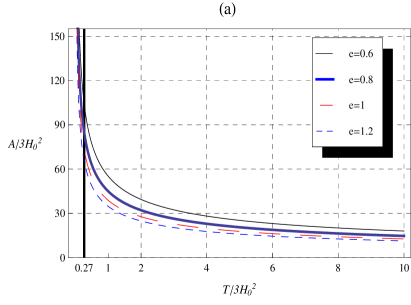
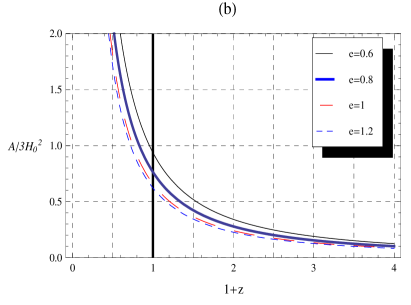
Figure 1: (Colour online) Evolution of $A(T)$ in HDE (a) versus $T$ (b) versus $z$ for different values of parameter $e$. Black thick line represents the current value of $T=T_{0}$. We set $\Omega_{M0}=0.27$, $\Omega_{\vartheta 0}=1-\Omega_{M0}$ and $H_{0}=74$.

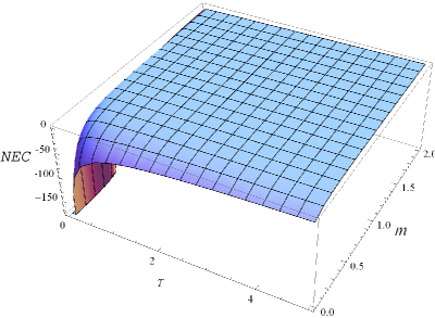
Figure 2: (Colour online) Evolution of NEC in HDE versus $T$ and $m$.

In this representation, we normalize $A(T)$ and $T$ to $3H_{0}^{2}$ and set $\Omega_{M0}=0.27$ and $e=0.6,0.8,1,1.2$. The function $A(T)$ is plotted against $T$ and $z$ in Figure 1. The difference among the values of $e$ is apparent for earlier times of the universe which vanishes in late times. Figure 1(b) shows the evolution in terms of redshift and here variation in curves is evident in future evolution for different values of $e$. The function $A(T)$ satisfies the EoS parameter $\omega_{dc}=-1-\frac{2}{3m}$ which depicts the phantom era of DE. Figure 2 clearly shows that for this $A(T)$ model, null energy condition (NEC) is violated and hence accelerated expansion of the universe is achievable. Here, NEC would violate even if one increases the value of $m$ which is in agreement with EoS parameter $\omega_{dc}$ for this model.

• $B(R)+{\lambda}T$

Here, we reconstruct the function $B(R)$ in the setting of HDE. For the choice of Hubble parameter $H(t)=\frac{m}{t_{p}-t}$, the future event horizon and matter energy density can be rewritten in terms of the Ricci scalar as

$$R_{\hat{E}}=\frac{1}{m+1}\sqrt{\frac{6m(2m+1)}{R}},\quad\rho_{M}=\frac{M^{2}_{p}[e^{2}(m+1)^{2}-m^{2}]}{2m(2m+1)}R.$$ (34)

Using Eqs.(18) and (23), one can get

$$(1+\omega_{\vartheta})\rho_{\vartheta}=\frac{M^{2}_{p}e^{2}(m+1)^{2}}{3m^{2}(2m+1)}R.$$ (35)

Substituting Eqs.(34) and (35) in Eq.(17) and solving, it follows that

$$B(R)=\mu_{-}R^{\jmath_{-}}C_{1}+\mu_{+}R^{\jmath_{+}}C_{2}+\gamma{R}+C_{3},$$ (36)

where

$$\jmath_{\pm} = \frac{1}{4}\left[3+m\pm\sqrt{m^{2}-10m+1}\right],\quad\quad\mu_{\pm}=\frac{1}{\jmath_{\pm}},$$

$$\gamma = \frac{(2-3{\lambda}m)}{2m^{2}}\left[m^{2}-e^{2}(m+1)^{2}\right],$$

$C_{1},~{}C_{2}$ and $C_{3}$ are constants.

Now, we define necessary initial conditions to determine the values of constants. For this purpose, we make the same assumption as in ref.¹⁷⁾. In particular, we choose the initial conditions $(B_{R})_{t=t_{0}}=1$ and $(B_{RR})_{t=t_{0}}=0$ which can be translated as

$$\left(\frac{dB}{dt}\right)_{t=t_{0}}=\left(\frac{dR}{dt}\right)_{t=t_{0}},\quad\left(\frac{d^{2}B}{dt^{2}}\right)_{t=t_{0}}=\left(\frac{d^{2}R}{dt^{2}}\right)_{t=t_{0}}.$$ (37)

Evaluating Eqs.(9) and (15), at $t=t_{0}$ and solving with respect to $B(R_{0})$, we ultimately have

$$B(t=t_{0})=R_{0}+\beta,\quad\beta=6H_{0}^{2}(1-\Omega_{M0}-\frac{3}{2}{\lambda}M^{2}_{p}\Omega_{M0}).$$ (38)

Applying the above initial conditions to the solution (36), it follows that

$$B(R)=C_{+}R^{\jmath_{+}}+C_{-}R^{\jmath_{-}}+\gamma{R}+\delta,$$ (39)

where

$$C_{+}=\frac{(\gamma-1)(\jmath_{-}-1)}{\jmath_{+}(\jmath_{+}-\jmath_{-})R_{0}^{\jmath_{+}-1}},\quad C_{-}=\frac{(\gamma-1)(\jmath_{+}-1)}{\jmath_{-}(\jmath_{-}-\jmath_{+})R_{0}^{\jmath_{-}-1}},$$

$$\delta=\beta+(1-\gamma)R_{0}+\frac{1}{\jmath_{+}\jmath_{-}}(\gamma-1)(\jmath_{+}+\jmath_{-}-1)R_{0}.$$

Consequently, the $f(R,T)$ model corresponding to HDE turns out to be

$$f(R,T)=C_{+}R^{\jmath_{+}}+C_{-}R^{\jmath_{-}}+\gamma{R}+\delta+{\lambda}T.$$ (40)

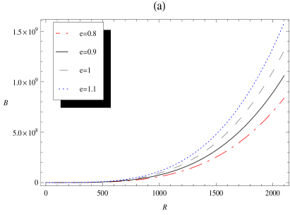
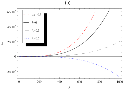
Figure 3: (Colour online) Evolution of $B(R)$ versus $R$ in HDE for (a) different values of $e$ with $\lambda=0$ and (b) different values of $\lambda$ with $e=1$.

We plot the function $B(R)$ against $R$ for different choices of parameters $e$ and $\lambda$. In Figure 3(a), we fix $\lambda=0$ (i.e., purely $f(R)$ gravity), which represents the variation of $B$ for different values of parameter $e$. It is obvious that curves become distinct for large $R$ and show increasing behavior. The effect of coupling parameter $\lambda$ is shown in Figure 3(b) for $e=1$. We can see that non-zero values of $\lambda$ modify the evolutionary nature of curves. We have also represented these results in terms of redshift in Figure 4. These curves exhibit the future evolution of $B$ for different values of parameters $e$ and $\lambda$.

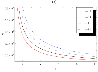
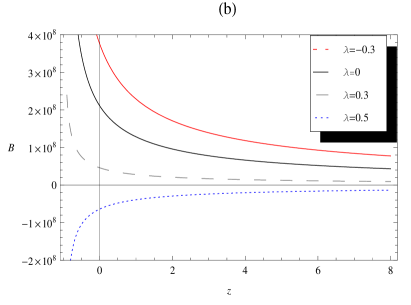
Figure 4: (Colour online) Evolution of $B(R)$ versus $z$ in HDE for (a) different values of $e$ with $\lambda=0$ and (b) different values of $\lambda$ with $e=1$.

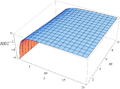
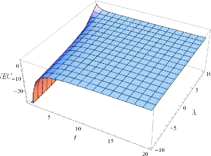
Figure 5: (Colour online) Evolution of NEC for $B(R)$ in HDE (a) with $\lambda=0.1$ and varying $m$ (b) with $m=10$ and varying $\lambda$.

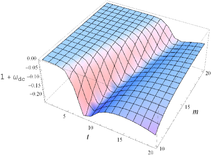
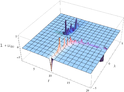
Figure 6: (Colour online) Evolution of $1+\omega_{dc}$ for $B(R)$ in HDE (a) with $\lambda=0.1$ and varying $m$ (b) with $m=10$ and varying $\lambda$.

We also explore the behavior of NEC for the reconstructed $B(R)$ in HDE and display the graphs for different values of parameters $m$ and $\lambda$. Figure 5 shows that NEC is violated i.e., $\rho_{dc}+p_{dc}<0$ which necessitates $\omega_{dc}<-1$. To make sure the phantom regime of the DE, we also plot the evolution of $1+\omega_{dc}$ against $m$ and $\lambda$ shown in Figure 6. The plots clearly favors the accelerated expansion except for particular range of $\lambda$. Thus the $f(R,T)$ model corresponding to HDE is consistent with present day observations^1-2).

4 Reconstruction from New Agegraphic Dark Energy

In this section, we discuss the reconstruction of $f(R,T)$ gravity in the setting of NADE. The energy density of NADE is proposed as ³⁰⁾

$$\rho_{\vartheta}=\frac{3n^{2}M^{2}_{p}}{\xi^{2}},$$ (41)

where the numerical component $3n^{2}$ is inserted to parameterize some uncertainties namely, the specific forms of cosmic quantum fields and the role of curvature of spacetime etc., $\xi$ is the conformal time in FRW background defined as

$$\xi=\int{\frac{dt}{a(t)}}=\int{\frac{da}{Ha^{2}}}.$$

Wei and Cai³⁰⁾ developed the cosmological constraints on NADE and found that the resolution of coincidence problem may become more definite in the NADE model with specific value of $n$ nearly unity. They constrained the NADE by using the observational data of SNeIa, CMB and LSS and found the best fit parameter (with $1\sigma$ uncertainty) $n=2.76^{+0.111}_{-0.109}$. The new agegraphic DE has been under consideration in both GR and modified theories scenario³¹⁾. The time derivative of $\rho_{\vartheta}$ is obtained as

$$\dot{\rho}_{\vartheta}=\frac{-2\rho_{\vartheta}H\sqrt{\Omega_{\vartheta}}}{an}.$$ (42)

Substituting Eq.(42) in Eq.(21), it follows that

$$\omega_{\vartheta}=-1+\frac{2}{3n}\frac{\sqrt{\Omega_{\vartheta}}}{a}.$$ (43)

We are concerned to demonstrate the possible correspondence between $f(R,T)$ models and NADE. In the following, we discuss the two cases individually.

• $R+2A(T)$

Comparing Eqs.(43) and (13), we obtain

$$TA_{T}-\frac{\sqrt{\Omega_{\vartheta}}}{3na-2\sqrt{\Omega_{\vartheta}}}A=0.$$ (44)

For $a(t)=a_{0}(t_{p}-t)^{-m}$, its solution is $A(T)=C_{4}T^{K_{1}}$, where $C_{4}$ is constant of integration and $K_{1}=(m+1)/(m-2)$. Now, we develop initial constraint on $A(T)$ for NADE model and find out the constant $C_{4}$. Evaluating Eq.(44) at present day and manipulating with Eq.(30), we obtain the following initial condition on $A(T)$

$$A(T_{0})=3H_{0}^{2}{\Omega}_{\vartheta 0}\left(1+\frac{2\sqrt{\Omega_{\vartheta 0}}}{3na_{0}-2\sqrt{\Omega_{\vartheta 0}}}\right)^{-1}.$$ (45)

Making use of Eq.(45) and relation $A(T)=C_{4}T^{K_{1}}$, the $f(R,T)$ model is constructed as

$$f(R,T)=R+6H_{0}^{2}{\Omega}_{\vartheta 0}T_{0}^{-K_{1}}\left(1+\frac{2\sqrt{\Omega_{\vartheta 0}}}{3na_{0}-2\sqrt{\Omega_{\vartheta 0}}}\right)^{-1}T^{K_{1}}.$$ (46)

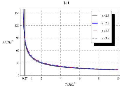
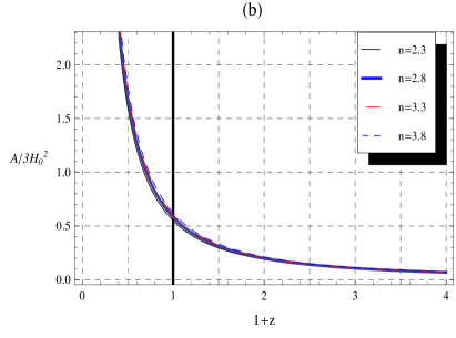
Figure 7: (Colour online) Evolution of $A(T)$ in NADE (a) versus $T$ and (b) versus $z$ for different values of $n$. Black thick line represents the current value of $T=T_{0}$.

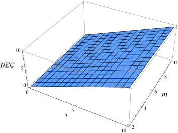
Figure 8: (Colour online) Evolution of NEC in NADE versus $T$ and $m$.

In case of NADE, we set $n=2.3,2.8,3.3,3.8$ and plot $A(T)$ in terms of $T$ and redshift as shown in Figure 7. One can see that the difference in evolutionary curves of $A(T)$ depending on the value of $n$ is not obvious in both graphs. These plots represent the future era where $A(T)$ is increasing rapidly. The EoS of DE components for the $A(T)$ model (46) is found as $\omega_{dc}=-1+\frac{2(m+1)}{3m}$ which represents the quintessence era of DE. We also plot the NEC for this $A(T)$ model by varying the values of parameter $m$ shown in Figure 8. The NEC is found to be satisfied i.e., $\rho+p>0$ which confirms the regime with $\omega_{dc}>-1$. Hence, the reconstructed $A(T)$ for NADE represents the quintessence era of the universe.

• $B(R)+{\lambda}T$

The conformal time $\xi$ of FRW universe can be represented in terms of Ricci scalar $R$ as

$$\xi=\frac{1}{a_{0}(m+1)}\left[\frac{6m(2m+1)}{R}\right]^{\frac{m+1}{2}}.$$

Likewise $\rho_{M}$ and $(1+\omega_{\vartheta})\rho_{\vartheta}$ for NADE are determined as

$$\rho_{M}=\frac{3M^{2}_{p}[n^{2}a^{2}_{0}(m+1)^{2}(-1)^{m}R^{m}-m^{2}(6m(2m+1))^{m}]}{[6m(2m+1)]^{m+1}}R,$$ (47)

$$(1+\omega_{\vartheta})\rho_{\vartheta}=\frac{2n^{2}a_{0}^{2}M^{2}_{p}(m+1)^{3}(-1)^{m+1}}{m[6m(2m+1)]^{m+1}}R^{m+1}.$$ (48)

Solving the differential equation (17) for NADE, it follows that

$$B(R)=\mu_{-}R^{\jmath_{-}}C_{5}+\mu_{+}R^{\jmath_{+}}C_{6}+\chi{R}^{m}+\gamma{R}+C_{7},$$ (49)

where $\gamma$ and $\chi$ are given by

$$\gamma = \frac{1}{2m}[2m-3\lambda{M_{p}^{2}}m^{2}],$$

$$\chi = \frac{n^{2}a_{0}^{2}(m+1)(-1)^{m+1}[3\lambda{M^{2}_{p}}m+2(m+1)]}{2(m^{3}+2m^{2})[6m(2m+1)]^{m}}.$$

Here, constants $C_{5},~{}C_{6}$ and $C_{7}$ can be determined from the initial conditions (37) and (38). The resulting NADE model of the Lagrangian $B(R)+{\lambda}T$ is

$$f(R,T)=\chi{R}^{m}+C_{+}R^{\jmath_{+}}+C_{-}R^{\jmath_{-}}+\gamma{R}+\delta+{\lambda}T,$$ (50)

where

$$C_{+} = \frac{(\gamma-1)(\jmath_{-}-1)R_{0}+\chi{m}(\jmath_{-}-m)\chi{R}_{0}^{m}}{\jmath_{+}(\jmath_{+}-\jmath_{-})R_{0}^{\jmath_{+}}},$$

$$C_{-} = \frac{(\gamma-1)(\jmath_{+}-1)R_{0}+\chi{m}(\jmath_{+}-m)\chi{R}_{0}^{m}}{\jmath_{-}(\jmath_{-}-\jmath_{+})R_{0}^{\jmath_{-}}},$$

$$\delta = \beta+(1-\gamma)R_{0}-\chi{R_{0}}^{m}+\frac{1}{\jmath_{+}\jmath_{-}}\left[(\gamma-1)(\jmath_{+}+\jmath_{-}-1)R_{0}\right.$$

$$+ \left.m\chi(\jmath_{+}+\eta_{-}-1)R_{0}^{m}\right].$$

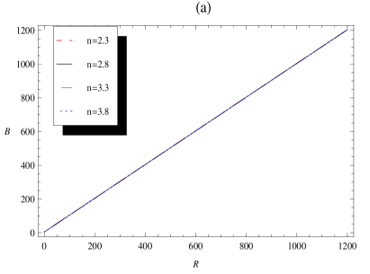
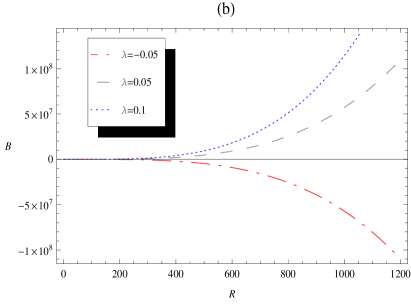
Figure 9: (Colour online) Evolution of $B(R)$ versus $R$ in NADE for (a) different values of $n$ with $\lambda=0$ and (b) different values of $\lambda$ with $n=2.8$.

For the NADE, the function $B(R)$ is plotted against $R$ for different values of parameter $n$ and $\lambda$ as shown in Figure 9. In Figure 9(a), we fix $\lambda=0$ (corresponds to $f(R)$ gravity) and represent the behavior of $B(R)$ for different values of $n$. It shows that the curves for reconstructed $B(R)$ in NADE are same. If one introduces the coupling parameter $\lambda$ with $n=2.8$, the variation in results is evident from Figure 9(b). We also plot these results in $B-z$ plane and represent the future evolution of $B(R)$ as shown in Figure 10.

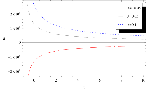
Figure 10: (Colour online) Evolution of $B(R)$ versus $z$ in NADE.

Now we check the validity of NEC for the $B(R)$ in NADE shown in Figure 11. It is clear that NEC is satisfied i.e., $\rho_{dc}+p_{dc}>0$ except for the negative values of coupling parameter $\lambda$. Consequently, these models should imply $\omega_{dc}>-1$, the quintessence EoS parameter. We show the evolution of $1+\omega_{dc}$ for different values of parameters $m$ and $\lambda$. The plots in Figure 12 make it more definite that the reconstructed function $B(R)$ favors the quintessence regime of the universe.

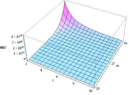
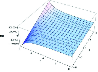
Figure 11: (Colour online) Evolution of NEC for $B(R)$ in NADE (a) with $\lambda=0.1$ and varying $m$ (b) with $m=10$ and varying $\lambda$.

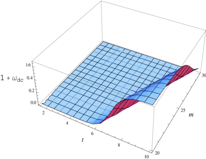
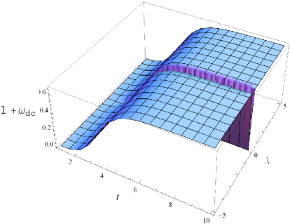
Figure 12: (Colour online) Evolution of $1+\omega_{dc}$ for $B(R)$ in NADE (a) with $\lambda=0.1$ and varying $m$ (b) with $m=10$ and varying $\lambda$.

5 Generalized Second Law of Thermodynamics

Here, we discuss the validity of GSLT in this modified gravity on the future event horizon. The GSLT states that entropy of a black hole horizon summed to the entropy of matter and fluids inside the horizon is non-decreasing with time. The validity of GSLT has been discussed in the setting of modified theories of gravity ^32-34). In¹⁵⁾, a non-equilibrium picture of thermodynamics is discussed on the apparent horizon of FRW spacetime in $f(R,T)$ gravity. It is remarked that usual laws of thermodynamics do not hold in this modified theory and additional entropy production term $\hat{S}_{\jmath}$ is required. We consider a flat FRW universe consisting of ordinary matter plus the DE component. The modified first law of thermodynamics is stated as¹⁵⁾

$$T_{h}d\hat{S}_{in}=Vd\rho_{EFF}+(\rho_{EFF}+p_{EFF})dV-T_{h}d\hat{S}_{\jmath},$$ (51)

where $T_{h}$ and $\hat{S}_{in}$ represent temperature and entropy of entire contents within the horizon. We have to show that

$$\dot{\hat{S}}=\dot{\hat{S}}_{h}+\dot{\hat{S}}_{in}+\dot{\hat{S}}_{\jmath}\geqslant 0,$$ (52)

where $\hat{S}_{h}$ is the horizon entropy. For $V=4\pi{R}_{\hat{E}}^{3}/3$, Eq.(51) yields

$$T_{h}\dot{\hat{S}}_{in}=\frac{4}{3}\pi{R}_{\hat{E}}^{3}\dot{\rho}_{EFF}+4\pi(\rho_{EFF}+p_{EFF})\dot{R}_{\hat{E}}\dot{R}_{\hat{E}}-T_{h}\dot{\hat{S}}_{\jmath},$$ (53)

We assume that temperature $T_{h}$ is proportional to Gibbson-Hawking temperature^33,35)

$$T_{h}=\frac{lH}{2\pi},$$ (54)

where $l$ is a real constant. In the following, we study GSLT for two forms of $f(R,T)$ function.

• $f(R,T)=R+2A(T)$

In GR, the Bekenstein-Hawking entropy is given by the relation $\hat{S}_{h}=\hat{A}/4G$, where $\hat{A}=4{\pi}R_{\hat{E}}^{2}$ represents the area of the event horizon³⁶⁾. It was proposed that the horizon entropy is associated with Noether charge in the context of modified gravity theories³⁷⁾. Brustein et al. ³⁸⁾ interpreted that Wald entropy is equivalent to one-fourth of the horizon area with gravitational coupling being the effective one. Hence, the entropy in this modified gravity is defined as ¹⁵⁾

$${\hat{S}}_{h}=\frac{\hat{A}}{4G_{EFF}},\quad G_{EFF}=G+2A_{T}/8\pi,$$ (55)

its time rate is

$$\dot{\hat{S}}_{h}=\left(2\pi{R}_{\hat{E}}\dot{R}_{\hat{E}}+\pi{R}_{\hat{E}}^{2}\frac{d}{dt}\right)\frac{1}{G_{EFF}}.$$ (56)

Using the FRW equations for this $f(R,T)$ model, Eq.(53) leads to

$$\dot{\hat{S}}_{in}+\dot{\hat{S}}_{\jmath}=\frac{2\pi{R}_{\hat{E}}^{2}}{lH}\left(\dot{H}+\frac{H^{2}R_{\hat{E}}}{2}\frac{d}{dt}\right)\frac{1}{G_{EFF}},$$ (57)

Thus, the total entropy for GSLT becomes

$$\dot{\hat{S}}=\frac{\pi{R}_{\hat{E}}^{2}}{G_{EFF}}\left[2\left(\frac{\dot{R}_{\hat{E}}}{{R}_{\hat{E}}}+\frac{\dot{H}}{lH}\right)-\left(1+\frac{HR_{\hat{E}}}{l}\right)\frac{\dot{G}_{EFF}}{G_{EFF}}\right]\geqslant 0,$$ (58)

or equivalently

$$\dot{\hat{S}}=\frac{2\pi{R}_{\hat{E}}^{2}}{G_{EFF}}\left[\frac{d}{dt}[ln(R_{\hat{E}}H^{1/l})]+\ln e^{(1+\frac{HR_{\hat{E}}}{l})}\frac{d}{dt}[\ln\frac{1}{\sqrt{G_{EFF}}}]\right]\geqslant 0.$$ (59)

In GR, the above condition reduces to $(R_{\hat{E}}H^{1/l})\geqslant 0$. The effective gravitational coupling constant for this $f(R,T)$ model needs to be positive so that $A_{T}>0$. To illustrate our result, let us consider the $f(R,T)$ model given by Eq.(33). In this model, $H=\frac{m}{(t_{p}-t)}$, $\dot{H}=\frac{m}{t_{p}-t}$ and $R_{\hat{E}}=\frac{(t_{p}-t)}{(m+1)}$. By the direct replacement of these results, we obtain that GSLT is valid if $l\leqslant 1$, $A_{T}>0$ and $\dot{A}_{T}\leqslant 0$. For $A(T)=3H_{0}^{2}{\Omega}_{\vartheta 0}T_{0}^{-K}\left(1+2\frac{e-\sqrt{\Omega_{\vartheta 0}}}{e+2\sqrt{\Omega_{\vartheta 0}}}\right)^{-1}T^{K}$, the condition $A_{T}>0$ holds if $3H_{0}^{2}{\Omega}_{\vartheta 0}T_{0}^{-K}\left(1+2\frac{e-\sqrt{\Omega_{\vartheta 0}}}{e+2\sqrt{\Omega_{\vartheta 0}}}\right)^{-1}<(3m+2){T}^{1-K}$ and $\dot{A_{T}}<0$, since $\dot{A_{T}}=\dot{T}K(K-1)3H_{0}^{2}{\Omega}_{\vartheta 0}T_{0}^{-K}\left(1+2\frac{e-\sqrt{\Omega_{\vartheta 0}}}{e+2\sqrt{\Omega_{\vartheta 0}}}\right)^{-1}T^{K-2}$ with $\dot{T}=\dot{\rho}<0$.

• $f(R,T)=B(R)+{\lambda}T$

For this specific model, the Wald entropy is defined as¹⁵⁾

$$\hat{S}_{h}=\frac{\hat{A}B_{R}}{4\tilde{G}},\quad\tilde{G}=G+\lambda/8\pi,$$ (60)

whose time derivative gives

$$\dot{\hat{S}}_{h}=\left(2\pi{R}_{\hat{E}}\dot{R}_{\hat{E}}B_{R}+\pi{R}_{\hat{E}}^{2}\dot{B_{R}}\right)\frac{1}{\tilde{G}}.$$ (61)

Following the above procedure, the GSLT leads to

$$\frac{2\pi{R}_{\hat{E}}^{2}B_{R}}{\tilde{G}}\left[\frac{d}{dt}[\ln(R_{\hat{E}}H^{1/l})]+\ln e^{(1+\frac{HR_{\hat{E}}}{l})}\frac{d}{dt}[\ln\sqrt{B_{R}}]\right]\geqslant 0.$$ (62)

For the particular choice of scale factor $a(t)=a_{0}(t_{p}-t)^{-m}$ with $R=\frac{-6m(2m+1)}{(t_{p}-t)^{2}}$, we consider the $f(R,T)=B(R)+{\lambda}T$ model (40) corresponding to HDE. The GSLT would be valid if $l\leqslant 1$ and scalar curvature lies in the range $\frac{-\gamma{R}^{1-\jmath_{-}}-C_{-}\jmath_{-}}{C_{+}\jmath_{+}}<R^{\jmath_{+}-\jmath_{-}}<\frac{C_{-}\jmath_{-}(1-\jmath_{-})}{C_{+}\jmath_{+}(\jmath_{+}-1)}$.

6 Conclusions

The $f(R,T)$ theory can be reckoned as a useful candidate of dark energy components which may help to understand the accelerated expansion of the universe. In such theory, cosmic acceleration may appear as an outcome of unified contribution from geometrical and matter components. We have discussed the cosmological reconstruction of $f(R,T)$ theory in the light of holographic and new agegraphic DE models. There are various models of $f(R,T)$ Lagrangian¹⁴⁾ but we have concentrated on $f(R,T)=f_{1}(R)+f_{2}(T)$ with particular functions $f_{1}$ and $f_{2}$. The model $f(R,T)=R+2A(T)$ matches the usual Einstein action plus time dependent cosmological constant which is presented as function of trace of the energy-momentum tensor. One can see that if the contribution of curvature matter coupling is null, i.e., $A(T)=0$ then the model reduces to GR which represents the matter dominated universe. The second model $f(R,T)=B(R)+{\lambda}T$ appears as matter corrected $f(R)$ type gravity.

We have formulated the field equations for each model in flat FRW background and obtained the evolution equation for the respective unknown functions. The HDE and NADE models are proposed as an equivalent description to DE components originating from the stated modified theory. Some analytical solutions have been obtained by applying the initial conditions on respective functions. Accordingly, one can determine the explicit $f(R,T)$ functions corresponding to HDE and NADE.

For HDE dominated universe, i.e., $\Omega_{\vartheta}\thicksim 1$; if $e>1$ then expansion is in quintessence regime and Eq.(25) implies that $A(T)\propto{T}^{\alpha},~{}\alpha>0,~{}e=1$ leading to the de Sitter universe with $A(T)\propto{constant}$. When $e<1$, phantom evolution of the universe is on cards with $A(T)\propto{T}^{\alpha},~{}\alpha<0$. The reconstructed $A(T)$ model satisfies the EoS parameter $\omega_{dc}<-1$ which is evident from Figure 2. For the model $f(R,T)=B(R)+{\lambda}T$, we discuss the evolution of $B(R)$ and explore the behavior of NEC and $1+\omega_{dc}$. The NEC is found to be violated which results in $\omega_{dc}<-1$ as depicted in Figures 5 and 6. Thus the $f(R,T)$ models reconstructed for HDE represent the phantom era of DE which is consistent with the recent observations^1,2).

In case of NADE having $\Omega_{\vartheta}\thicksim 1$, the EoS parameter $\omega_{\vartheta}=-1+\frac{2}{3n}\frac{\sqrt{\Omega_{\vartheta}}}{a}$ can be less than $-1$ if $n<0$ but from observational point of view $n=2.76^{+0.111}_{-0.109}$³⁰⁾ which permits the quintessence era and the corresponding $A(T)$ model is of the form $A(T)\propto{T}^{\frac{1}{3na-1}}$. The EoS parameter corresponding to $A(T)$ represents the quintessence regime of DE which constitutes the relation $\rho_{dc}+p_{dc}>0$ as depicted in Figure 8. The evolution of the function $B(R)$ corresponding to NADE $f(R,T)$ model is discussed in Figures 9-12. These plots show the influence of coupling parameter $\lambda$ on the evolutionary regime of the universe. We find that function $B(R)$ for the NADE favors the quintessence era of the DE.

The EoS parameter $\omega_{dc}$ for the above $f(R,T)$ models is in agreement with the observational data of WMAP5³⁹⁾. Hence, we can suggest that these reconstructed models of $f(R,T)$ gravity are consistent with the evolution of HDE and NADE in general relativity. The polynomial functions (40) and (50) represent more general $f(R,T)$ models of the type $B(R)+{\lambda}T$. If one puts $\lambda=0$ then the respective models in $f(R)$ gravity can be reproduced. Though $f(R)$ theory has been reconstructed for HDE and NADE but these functions appear to be more general. We have also assured the validity of GSLT on the future event horizon of FRW universe. The HDE $f(R,T)$ models are employed to establish the constraints which validate the GSLT in this modified gravity.

Acknowledgment

We would like to thank the Higher Education Commission, Islamabad, Pakistan for its financial support through the Indigenous Ph.D. 5000 Fellowship Program Batch-VII. The authors are grateful to the Physical Society of Japan for Financial Support in publication
1) S. Perlmutter, S. Gabi, G. Goldhaber, A. Goobar, D. E. Groom, I. M. Hook, A. G. Kim, M. Y. Kim, G. C. Lee, R. Pain, C. R. Pennypacker, I. A. Small, R. S. Ellis, R. G. McMahon, B. J. Boyle, P. S. Bunclark, D. Carter, M. J. Irwin, K. Glazebrook, H. J. M. Newberg, A. V. Filippenko, T. Matheson, M. Dopita and W. C. Couch: Astrophys. J. 483 (1997) 565; A. G. Riess, L. G. Strolger, J. Tonry, Z. Tsvetanov, S. Casertano, H. C. Ferguson, B. Mobasher, P. Challis, N. Panagia, A. V. Filippenko, W. Li, R. Chornock, R. P. Kirshner, B. Leibundgut, M. Dickinson, A. Koekemoer, N. A. Grogin and M. Giavalisco : Astrophys. J. 607 (2004) 665.
2) C. L. Bennett, M. Halpern, G. Hinshaw, N. Jarosik, A. Kogut, M. Limon, S. S. Meyer, L. Page, D. N. Spergel, G. S. Tucker, E. Wollack, E. L. Wright, C. Barnes, M. R. Greason, R. S. Hill, E. Komatsu, M. R. Nolta, N. Odegard, H. V. Peiris, L. Verde and J. L. Weiland: Astrophys. J. Suppl. 148 (2003) 1; D. N. Spergel, R. Bean, O. Dor , M. R. Nolta, C. L. Bennett, J. Dunkley, G. Hinshaw, N. Jarosik, E. Komatsu, L. Page, H. V. Peiris, L. Verde, M. Halpern, R. S. Hill, A. Kogut, M. Limon, S. S. Meyer, N. Odegard, G. S. Tucker, J. L. Weiland, E. Wollack and E. L. Wright: Astrophys. J. Suppl. 170 (2007) 377.
3) E. Hawkins, S. Maddox, S. Cole, O. Lahav, D. S. Madgwick, P. Norberg, J. A. Peacock, I. K. Baldry, C. M. Baugh, J. Bland-Hawthorn, T. Bridges, R. Cannon, M. Colless, C. Collins, W. Couch, G. Dalton, R. D. Propris, S. P. Driver, S. P., G. Efstathiou, R. S. Ellis, C. S. Frenk, K. Glazebrook, C. Jackson, B. Jones, I. Lewis, S. Lumsden, W. Percival, B. A. Peterson, W. Sutherland and K. Taylor: Mon. Not. Roy. Astron. Soc. 346 (2003) 78; M. Tegmark, M. A. Strauss, M. R. Blanton, K. Abazajian, S. Dodelson, H. Sandvik, X. Wang, D. H. Weinberg, I. Zehavi, N. A. Bahcall, F. Hoyle, D. Schlegel, R. Scoccimarro, M. S. Vogeley, A. Berlind, T. Budavari, A. Connolly, D. J. Eisenstein, D. Finkbeiner, J. A. Frieman, J. E. Gunn, L. Hui, B. Jain, D. Johnston, S. Kent, H. Lin, R. Nakajima, R. C. Nichol, J. P. Ostriker, A. Pope, R. Scranton, U. Seljak, R. K. Sheth, A. Stebbins, A. S. Szalay, I. Szapudi, Y. Xu, J. Annis, J. Brinkmann, S. Burles, F. J. Castander, I. Csabai, J. Loveday, M. Doi, M. Fukugita, B. Gillespie, G. Hennessy, D. W. Hogg, Z. E. Ivezic , G. R. Knapp, D. Q. Lamb, B. C. Lee, R. H. Lupton, T. A. McKay, P. Kunszt, J. A. Munn, L. Connell, J. Peoples, J. R. Pier, M. Richmond, C. Rockosi, D. P. Schneider, C. Stoughton, D. L. Tucker, D. E. V. Berk, B. Yanny and D. G. York: Phys. Rev. D 69 (2004) 103501.
4) D. J. Eisentein, I. Zehavi, D. W. Hogg, R. Scoccimarro, M. R. Blanton, R. C. Nichol, R. Scranton, Hee-Jong Seo, M. Tegmark, Z. Zheng, S. F. Anderson, J. Annis, N. Bahcall, J. Brinkmann, S. Burles, F. J. Castander, A. Connolly, I. Csabai, M. Doi, M. Fukugita, J. A. Frieman, K. Glazebrook, J. E. Gunn, J. S. Hendry, G. Hennessy, Z. Ivezic’, S. Kent, G. R. Knapp, H. Lin, Yeong-Shang Loh, R. H. Lupton, B. Margon, T. A. McKay, A. Meiksin, J. A. Munn, A. Pope, M. W. Richmond, D. Schlegel, D. P. Schneider, K. Shimasaku, C. Stoughton, M. A. Strauss, M. SubbaRao, A. S. Szalay, I. Szapudi, D. L. Tucker, B. Yanny, and D. G. York: Astrophys. J. 633 (2005) 560.
5) B. Jain and A. Taylor: Phys. Rev. Lett. 91 (2003) 141302.
6) V. Sahni: Lect. Notes Phys. 653 (2004) 141; M. Sharif and M. Zubair: Int. J. Mod. Phys. D 19 (2010) 1957; M. Li, X.-D. Li, S. Wang and Y. Wang: Commun. Theor. Phys. 56 (2011) 525; K. Bamba, S. Capozziello, S. Nojiri and S. D. Odintsov: Astrophys. Space Sci. 342 (2012) 155.
7) S. Weinberg: Rev. Mod. Phys. 61 (1989) 1; P. J. E. Peebles and B. Ratra: Rev. Mod. Phys. 75 (2003) 559.
8) L. Susskind: J. Math. Phys. 36 (1995) 6377.
9) A. G. Cohen, D. B. Kaplan and A. E. Nelson: Phys. Rev. Lett. 82 (1999) 4971.
10) M. Li: Phys. Lett. B 603 (2004) 1.
11) Q. G. Huang and Y. G. Gong: JCAP 0408 (2004) 006; X. Zhang and F.-Q. Wu: Phys. Rev. D 72 (2005) 043524; ibid. 76 (2007) 023502.
12) T. P Sotiriou and V. Faraoni: Rev. Mod. Phys. 82 (2010) 451; A. De Felice and S. Tsujikawa: Living Rev. Rel. 13 (2010) 3; S. Nojiri and S. D. Odintsov: Phys. Rep. 505 (2011) 59.
13) R. Ferraro and F. Fiorini: Phys. Rev. D 75 (2007) 08403; G. R. Bengochea and R. Ferraro: Phys. Rev. D 79 (2009) 124019; E. V. Linder: Phys. Rev. D 81 (2010) 127301.
14) T. Harko, F. S. N. Lobo, S. Nojiri and S. D. Odintsov: Phys. Rev. D 84 (2011) 024020.
15) M. Sharif and M. Zubair: JCAP 03 (2012) 028 [Erratum ibid. 05 (2012) E01].
16) M. Jamil, D. Momeni, M. Raza and R. Myrzakulov: Eur. Phys. J. C 72 (2012) 1999.
17) M. J. S. Houndjo and O. F. Piattella: Int. J. Mod. Phys. D 21 (2012) 1250024.
18) M. J. S. Houndjo: Int. J. Mod. Phys. D 21 (2012) 1250003.
19) M. Sharif and M. Zubair: J. Phys. Soc. Jpn. 81 (2012) 114005.
20) M. Sharif and M. Zubair: J. Phys. Soc. Jpn. 82 (2013) 014002.
21) S. Capozziello, V. F. Cardone and A. Troisi: Phys. Rev. D 71 (2005) 043503.
22) M. R. Setare: Int. J. Mod. Phys. D 17 (2008 )2219.
23) X. Wu and Z.-H. Zhu: Phys. Lett. B 660 (2008) 293.
24) C.-J. Feng: Phys. Lett. B 676 (2009) 168.
25) K. Karami and M. S. Khaledian: JHEP 03 (2011) 086.
26) M. H. Daouda, M. E. Rodrigues and M. J. S. Houndjo: Eur. Phys. J. C 72 (2012) 1893.
27) S. Carloni, R. Goswami and P. K. S. Dunsby: Class. Quantum Grav. 29 (2012) 135012.
28) L. D. Landau, and E. M. Lifshitz: The Classical Theory of Fields (Butterworth-Heinemann, 2002).
29) S. Nojiri, S. D. Odintsov and S. Tsujikawa: Phys. Rev. D 71 (2005) 063004; K. Bamba, R. Myrzakulov, S. Nojiri and S. D. Odintsov: Phys. Rev. D 85 (2012) 104036.
30) H. Wei and R. G. Cai: Phys. Lett. B 660 (2008) 113; ibid. 663 (2008) 1.
31) J.-P. Wu, D.-Z. Ma and Y. Ling: Phys. Lett. B 663 (2008) 152; A. Sheykhi: Phys. Rev. D 81 (2010) 023525; M. Jamil and E. N. Saridakis: JCAP 07 (2010) 028; M. R. Setare: Astrophys. Space Sci. 326 (2010) 27.
32) R. G. Cai and S. P. Kim: JHEP 02 (2005) 050; M. Akbar and R. G. Cai: Phys. Rev. D 75 (2007) 084003.
33) H. M. Sadjadi: Phys. Rev. D 76 (2007) 104024.
34) K. Bamba and C. Q. Geng: Phys. Lett. B 679 (2009) 282; JCAP 06 (2010) 014; ibid. 11 (2011) 008.
35) U. Debnath, S. Chattopadhyay, I. Hussain, M. Jamil and R. Myrzakulov: Eur. Phys. J. C 72 (2012) 1875.
36) J. D. Bekenstein: Phys. Rev. D 7 (1973) 2333.
37) R. M. Wald: Phys. Rev. D 48 (1993) 3427.
38) R. Brustein, D. Gorbonos and M. Hadad: Phys. Rev. D 79 (2009) 044025.
39) E. Komatsu, J. Dunkley, R. Nolta, C. L. Bennett, B. Gold, G. Hinshaw, N. Jarosik, D. Larson, M. Limon, L. Page, D. N. Sperge, M. Halpern, R. S. Hill, A. Kogut, S. S. Meyer, G. S. Tucker, J. L. Weiland, E. Wollack, and E. L. Wright: Astrophys. J. Suppl. 180 (2009) 330.