Strange Baryon to Meson Ratio

Abstract

We present a model to compute baryon and meson transverse momentum distributions, and their ratios, in relativistic heavy-ion collisions. The model allows to compute the probability to form colorless bound states of either two or three quarks as functions of the evolving density during the collision. The qualitative differences of the baryon to meson ratio for different collision energies and for different particle species can be associated to the different density dependent probabilities and to the combinatorial factors which in turn depend on whether the quarks forming the bound states are heavy or light. We compare to experimental data and show that we obtain a good description up to intermediate values of $pt$.

1 Introduction

Long time ago it has been proposed [1] that strangeness is easier produced in the QGP than in a hadronic environment. At the Large Hadron Collider (LHC), new results on strangeness production [2] are being obtained, among them are the transverse momentum distributions for pions, kaons, protons and $\Lambda$ as well as baryon to meson ratios. The distributions show disagreement with perturbative QCD results, especially on the strangeness sector. Consequently, the baryon to meson ratio presents an unexplained behavior at intermediate transverse momenta. The baryon to meson ratios measured at LHC energies could be different from the ratios measured at lower energies, since the former are driven predominantly by hard collisions. Many ideas have been developed to understand these ratios. Some studies include the percolation model [3], recombination [4], the statistical model [5], and also flow [6] in proton-proton collisions. The slight discrepancies of the statistical model with data provide the motivation to get further insight into the hadronization mechanism [7].

This work reports on an alternative model to study the production of hadrons in relativistic heavy ion collisions, where the evolving density during the collision and the strangeness abundance are key ingredients, the so called dynamical quark recombination model [8].

2 Transverse momentum distribution

The transverse momentum distributions are computed within the dynamical recombination model are given by

$$\frac{dN}{p_{T}dp_{T}dy} = g\frac{m_{T}}{4\pi}\frac{\rho_{\mbox{\tiny{nucl}}}^{2}}{\Delta\tau}\int_{\tau_{0}}^{\tau_{f}}\tau d\tau{\mathcal{P}}(\tau)I_{0}(p_{T}\sinh\eta_{T}/T)$$ (1)

$$\times \int d\eta\cosh(y-\eta)e^{-[m_{T}\cosh(y-\eta)\cosh\eta_{T}]/T}$$

where $\Delta\tau=\tau_{f}-\tau_{0}$ is the proper-time interval spanned during the hadron emission, $\eta_{T}$ is related to the transverse expansion velocity $\beta_{T}$ by $\beta_{T}=\tanh(\eta_{T})$, the temperature $T$ is given by the cooling law $T=T_{0}(\tau_{0}/\tau)^{v_{s}^{2}}$ and ${\mathcal{P}}$ is the probability of forming a given hadron as a function of proper-time $\tau$ and accounts for the fact that hadronization is not instantaneous. The profile of this probability can be obtained by Monte Carlo simulation (see Ref [8] for details). The spectrum given by Eq. (1), has $T$, $\beta_{T}$ and the overall normalization as the free parameters.

2.1 Combinatorial probabilities

The combinatorial analysis allows to estimate in a simple way the number of possible colorless baryons and mesons, when we take a certain number of heavy ($Q$) and light ($q$) quarks. Considering the case where one starts out with a set of $n$ $q$-quarks ($q=u,d$) and $m$ $Q$-quarks ($Q=s$), it is possible to form sets of two (mesons) or tree (baryons) quarks. The more simple case is when we have one $q$ and one $Q$ each comming in three colors. In that case the possible colorless combinations are show on the table 1. From this it is easy to compute the relative abundance of the mesons containing a $Q$ quark with respect to the total combinations, so the number of relative mesons is $2mn/(n+m)^{2}$. In a similar way, the total number of possible baryons plus antibaryons is $2(n+m)^{3}$, and the relative abundances of the baryons containing one $Q$ quark is $3n^{2}m/(n+m)^{3}$. In this way, one can compute the baryon to meson ratio as a function of the number of light ($n$) and heavy ($m$) quarks.

Table 1: Number of possible combination of 2 or 3 quarks

Kind	# of Mesons		kind	# of Baryons
$q\bar{q}$	$3n^{2}$		$qqq$	$n^{3}$
$q\bar{Q}$	$3nm$		$qqQ$	$3n^{2}m$
$Q\bar{q}$	$3nm$		$qQQ$	$3nm^{2}$
$Q\bar{Q}$	$3m^{2}$		$QQQ$	$m^{3}$

The previous exercise may be generalized for more light flavors, for instance, for the case of $q=u,d$ and $Q=s$. In this case, some of the combinations are $\Omega(sss)$ and $\Phi(s\bar{s})$. Considering an equal number ($n$) of $u$ and $d$ and $m$ as the number of $s$-quarks, we can estimate the ratio $\Omega/\Phi$ as,

$$\frac{\Omega}{\phi}=\frac{4m^{2}n+m^{2}}{8n^{3}+3n^{2}m+6nm^{2}}.$$ (2)

Since the strange quarks are produced in lesser quantities than up and down, we introduce the variable $x>1$ as $u=xs$ to write Eq. (2) as

$$\frac{\Omega}{\phi}=\frac{4x+1}{8x^{3}+3x^{2}+6x}.$$ (3)

This equation could be simplified even more, when ones takes only one light and one heavy flavor. Let us take for instance only $u$ and $s$ quarks, then Eq. (3) becomes

$$\frac{\Omega}{\phi}=\frac{1}{x+1}.$$ (4)

The behavior of the $\Omega/\Phi$ ratio as a function of the number of light and heavy flavors, described by Eq. (2), is shown in Fig. 2. For the case when we take $u=xs$ and the number of $u$’s is equal to the number of $d$’s, the baryon to meson ratio has the behavior shown with the dashed curve in Fig. 2. The case where there is only one heavy and one light quark ($d=0$), described by Eq. (4), is shown in the same figure with the solid curve. Notice that low values of $x$ correspond to higher collisions energies whereas high values correspond to less energetic collisions.

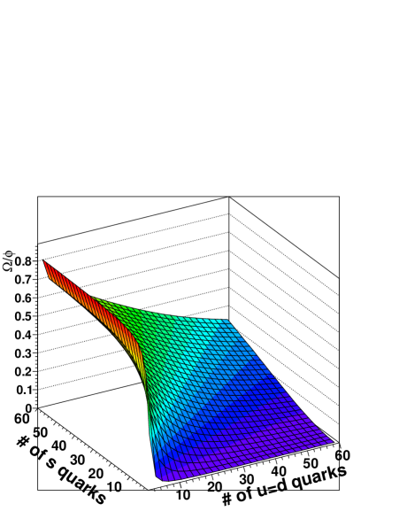
Figure 1: Ratio $\Omega/\Phi$ as function of the number of $s$ and light ($u=d$) quarks.

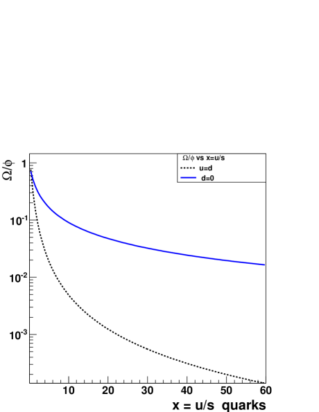
Figure 2: Ratio $\Omega/\phi$ as function of proportionality factor $x=u/s$ between light $u,d$ and $s$ quarks.

3 Results

In order to estimate the momentum distribution, we take an initial hadronization time, $\tau_{0}=1$ fm, and initial and final temperatures as 200 and 100 MeV respectively, which means a final hadronization time $\tau_{f}=8$ fm. Taking the $\Omega$ spectrum produced in Au+Au from STAR data [9] at 62.4 GeV, we can fit it and extract the transverse velocity $\beta_{T}$, as well as the normalization constant. The last parameters and the data on the ratio $\Omega/\Phi$ are used to extract the distribution of the $\Phi$, since this last one is not reported from experiment. The results are plotted in Fig. 4. Regarding the combinatorial probability and $p_{t}$ spectra, let us take into account the constrains on the probability ratios to form baryons and mesons, and the the fact that there is a proportionality factor $x$ between light and heavy quarks. Furthermore, taking into account the parameters of the fit and the constrains of the Eq. (4), it is possible to extract the proportionality factor $x$ between the number of light and heavy quarks. The top of Fig. 4 shows, the fitted spectra to $\Omega$ data and the prediction of the $\Phi$ spectrum. The bottom part shows the ratio fitted with three different values of the $x$. One can see that after $\approx$ 3 GeV our curves grow above data. This behavior could be explained as a consequence of the absence of the fragmentation and energy loss in our approach.

In summary, the dynamical recombination model together with constrains on the $\Omega/\phi$ ratio from combinatorial probabilities can describe RHIC data for Au+Au at two energies. We observe that the fits are better at low energy and lighter ions in the collisions. The constrains on the probabilities could provide a reasonable value for the proportionality between the number of light and heavy flavors, $x$.

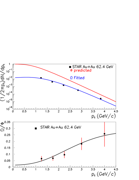
Figure 3: Experimental results of the spectra and the ratio $\Omega/\Phi$ fitted to the model and extracted the $\beta=0.40$

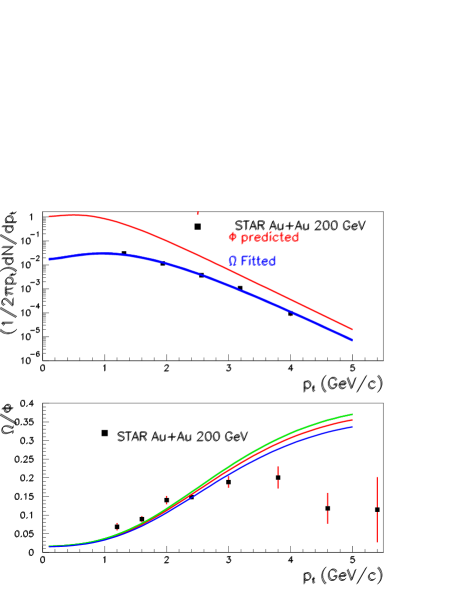
Figure 4: Spectra and ratio $\Omega/\phi$ fitted to the model and extracted the $\beta=0.45$, and the ratio for three values of $x$.

3.1 Acknowledgments

Support for this work has been received by CONACyT under grant numbers 101597 and 128534 and PAPIIT-UNAM under grant numbers IN107911 and IN103811.

References

References

- [1] J. Rafelski and B. Müller, Phys. Rev. Lett. 48, 1066 (1982).
- [2] B. Abelev, et. al. (ALICE Collaboration), Phys. Lett. B 712, 309 (2012); A. Aamodt, et al. (ALICE Collaboration), Eur. Phys. J. C 71, 1594 (2011).
- [3] I. Bautista, et al. Phys. Rev. C 82, 34912 (2010).
- [4] R. C. Hwa, et al. Phys. Rev. C 84, 64914 (2011); R. J. Fries, et al. Phys.Rev. Lett. 90, 202303 (2003).
- [5] S. Wheatron, et al. Comp. Phys. Comm. 180, 84 (2009); P. Braun, Phys. Lett. B 518, 41 (2001).
- [6] E. Cuautle and G. Paic, J. Phys. G 35, 075103 (2008); A. Ortiz, Velasquez, P. Christiansen, E. Cuautle Flores, I.A. Maldonado Cervantes, and G. Paic Phys. Rev. Lett. 111, 042001 (2013).
- [7] J. Cleymans, et. al. Phys. Rev. C 74, 34903 (2006).
- [8] A. Ayala, M. Matínez, G. Paic, G. Toledo-Sanchez, Phys. Rev. C 77, 044901 (2008); A. Ayala, J. Magnin, L.M. Montaño, G. Toledo-Sanchez, Phys. Rev. C 80, 064905 (2009).
- [9] M.M. Aggarwal, et al. (STAR Collaboration), Phys. Rev. C 83, 024901 (2011); G.M.S. Vasconcelos (for the STAR Collaboration) J. Phys. G 37, 094034 (2010).