Traffic Jams and Shocks of Molecular Motors inside Cellular Protrusions

Abstract

Molecular motors are involved in key transport processes inside actin-based cellular protrusions. The motors carry cargo proteins to the protrusion tip which participate in regulating the actin polymerization, and play a key role in facilitating the growth and formation of such protrusions. It is observed that the motors accumulate at the tips of cellular protrusions, and in addition form aggregates that are found to drift towards the protrusion base at the rate of actin treadmilling. We present a one-dimensional driven lattice model, where motors become inactive after delivering their cargo at the tip, or by loosing their cargo to a cargo-less neighbor. The results suggest that the experimental observations may be explained by the formation of traffic jams that form at the tip. The model is solved using a novel application of mean-field and shock analysis. We find a new class of shocks that undergo intermittent collapses, and on average do not obey the Rankine-Hugoniot relation.

The traffic of molecular motors is an example of a non-equilibrium process Kolomeisky and Fisher (2007). In order to describe the traffic of molecular motors the tools and theories of non-equilibrium statistical mechanics are useful Chou et al. (2011). In this letter we focus on the traffic of molecular motors inside actin-based cellular protrusions, such as filopodia and stereocilia. These protrusions are of a few microns in length and fractions of microns in diameter, and contain a polarized bundle of actin filaments Mattila and Lappalainen (2008). The actin polymerizes at the protrusion tip, such that it provides the force for the protrusion initiation, and treadmills (retrograde flow) at a constant rate when the protrusion reaches a steady-state shape.

Unconventional myosins bind and move processively toward the protrusion tip on these filaments, as shown in Fig. 1a. Experiments analyzing myosin traffic revealed that motors accumulate over a finite length scale from the tip in protrusions of different lengths, for example see Schneider et al. (2006). A striking phenomenon is seen in a variety of experiments with different types of myosin motors Berg and Cheney (2002); Belyantseva et al. (2005); Salles et al. (2009): The traffic of motors exhibit wave-trains, or ”pulses” of motor density, that move towards the base of the protrusion (opposite to the motors’ motion). The velocity of these aggregates is found to be close to that of the actin retrograde flow, suggesting that these are inactive or jammed motors. The theoretical challenge for a successful model is to explain both the finite length of the accumulation of motors at the tips of the protrusions, and to provide a mechanism for the pulse-like counter-propagating aggregates of motors.

The simplest description of motors along a linear track is in terms of a Total Asymmetric Exclusion Process (TASEP) Chou et al. (2011). We can model a protrusion as a half closed tube, open at its base to the cell cytoplasm (Fig.1a). Several works have dealt with this boundary condition (b.c.) together with attachment/detachment kinetics of the motors to the tracks Müller et al. (2005); Naoz et al. (2008); Zhuravlev et al. (2012). These models find that at steady-state the tubes are practically all jammed, and longer tubes have longer jammed (accumulation of motors) regions, in contrast with the observations for cellular protrusions. In Parmeggiani et al. (2003) it was shown that a track coupled to an infinite reservoir produces an accumulation with a fixed length for different system sizes (see Fig.S1, SI ). However it is unlikely that the confined volume of a cellular protrusion can serve as an infinite reservoir.

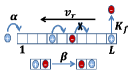
Figure 1: (Color online) (a) An illustration of a cellular protrusion. Myosin motors enter with probability $\alpha dt$ from the cell’s cytoplasm. They move on the actin track. Green ellipses are cargoes and without it the tail folds to inhibit the motor domain. (b) The model. Particles enter the first site with probability $\alpha dt$ an ’switch off’ only at the last site; there is no exit from the left. The track itself moves backward with probability $v_{r}dt$. Particles can exchange their mobility state. (c) Particles interaction. Particles can exchange cargoes and change their mobility state.

Similarly, the properties of the observed pulse-like aggregates of motors do not fit the traffic jams arising in TASEP. For example, It seems from experiments that the aggregates originate only at the protrusion tips, are rather stable while propagating and have low density regions between them. This is not what happens in TASEP where jams appear at the high density (HD) phase Schutz (2000), and jams appear everywhere. Sparse jams between free flow regions appear in models of vehicular traffic Schreckenberg et al. (1995), but they result from the combination of synchronous update and several particle velocities. There is no obvious reason why this should apply for molecular motors traffic.

To explain the observed phenomena we consider a generalization of TASEP as described in Fig. 1b. Each particle correspond to a molecular motor, and can be in one of two states: ’inactive’ where it is immobile on the actin track, and ’active’ where it can hop (move procssively along the actin filament). We note that internal degree of freedom was considered in the past Nishinari et al. (2005); Reichenbach et al. (2006); Klumpp et al. (2008); Pinkoviezky and Gov (2013). Motivated by experiments and theoretical models, we propose the following properties for the dynamics of the activity state of the motors: It was found that several types of molecular motors become processive only when they are bound to a cargo molecule Umeki et al. (2011); Manor et al. (2012). Since in many cases the cargo is involved in regulating the actin polymerization at the protrusion tip Tokuo and Ikebe (2004); Salles et al. (2009); Manor et al. (2011), we assume that the motors can only detach from the cargo at the tip and become inactive. When inactive, motors may detach from the actin filament, or stay attached Umeki et al. (2011) and drift towards the protrusion base due to the retrograde flow. Furthermore, neighboring motors can ”steal” the cargo from each other Manor et al. (2012), and this introduces a conservation of the activity whereby an inactive motor can only become active at the expense of a motor jammed behind it (Fig.1c). Such an interaction is known to produce a robust traffic-jam (condensate) Mallick (1996). Note that there are other forms of interactions among motors that result in their inactivation Quintero et al. (2010), and therefore our model may be treated as a coarse-grained description of more complex set of underlying interactions.

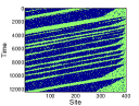
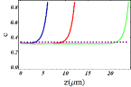
Figure 2: (Color online) (a) Kymograph. Green (bright) points are active particles while dark blue is the empty space. (b) Density profiles for systems of lengths $z=6,12,24\mu m$. Data is for $\alpha=\beta=0.05,v_{r}=0.1$ and $K_{f}=0.6/300$. Dashed purple curve is the theoretical bulk density $c_{b}$ (Eq.2,S4 SI ).

The parameters in our model are: $\bf 1)$ $K_{f}dt$ is the probability for a particle to switch from active to an inactive state at the tip (at the last site). $\bf 2)$ $\alpha dt$ is the probability that a particle enters the system at the left boundary (from the cell cytoplasm). $\bf 3)$ $\beta dt$ is the probability that an inactive motor followed by an active motor switch their mobility state (fig. 1c). $\bf 4)$ $v_{r}$ is the rate at which a new site (actin monomer) is added at the right end (tip) and simultaneously a site is removed at the left end. The actin retrograde velocity is therefore $v_{r}$, and we maintain a constant overall length of the protrusion which is assumed to be at steady-state. $\bf 5)$ We normalize the probabilities such that $dt$ is the hopping probability of an active particle.

The process defined above is the open b.c. version of a process with a single impurity particle on a ring Mallick (1996). In our process active motors enter from the left while impurity particles (inactive motors) enter from the right.

We show an example kymograph of the dynamics arising in our model in Fig. 2a. We find that near the tip there is a region of accumulation of motors, and large traffic jams are initiated there. Each traffic jam corresponds to an inactivation event of a motor at the tip, and these jams keep their size throughout the system as they move towards the left boundary. When a jam is formed, it transiently depletes the tip region, which gets refilled shortly afterwards. These properties of robust aggregates that form near the tip and deplete it, correspond qualitatively with the experimental observations of myosin-X Berg and Cheney (2002) and myosin-XV Belyantseva et al. (2005) in filopodia .

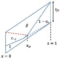
Figure 3: (Color online) (a) An example of a parallelogram (or slice) for $\alpha=0.2,\beta=0.05,v_{r}=0.1$ and $\Lambda_{f}=0.2$. (b) A description of a slice with the different density regions and the slopes connecting them (see SI for more examples). In both figures we see $x_{w}$ (Eq.1) where the densities [$c_{-},\beta,1-v_{r}$] meet.

We find in Fig. 2b that the accumulation length of the motors near the tip is independent of the system size. The spatial extent of each site corresponds to a motor step (i.e. $30nm$), therefore: $z=i\cdot 0.03\mu m$ where $i$ is the site number. We stress that without the switching mechanism the track would be uniformly occupied with density $1-v_{r}$ except for a shock on the left end. The jams initiated by the inactive particles determine a finite length of the accumulation region and do not let it grow to the system size. Such localized accumulations of motors are observed near the tips of stereocilia of different lengths Schneider et al. (2006), and our model suggests that this arises from the turnover of motors through the formation of jams.

We now turn to analyze the model in detail, at steady state. The interesting behavior arises in the regime where the inactivation rate $K_{f}$ is small, and significant accumulation of motors occurs at the tip. It is convenient to use the so-called ’mesoscopic scaling’ $K_{f}=\frac{\Lambda_{f}}{L}$ Reichenbach et al. (2006) and to use a spatial coordinate $x=\frac{i}{L},0\leq x\leq 1$, where $L$ is the number of sites in the system.

We start by comparing the numerical simulations to a naive mean field approximation (MFA) Derrida et al. (1992), which fails, as demonstrated in Fig. S2 SI . The reason for this deviation lies in the fact that the system separates into regions of different mean densities and currents. We therefore proceed with a detailed calculation of the average concentration profiles of the motors in our model, which is based on using MFA within each distinct region. We divide the whole space-time evolution of the system into parallelogram slices as shown in Fig. 3a. The $i$’th parallelogram is defined by $t_{fi}$ - the time between two successive inactivation events at the tip.

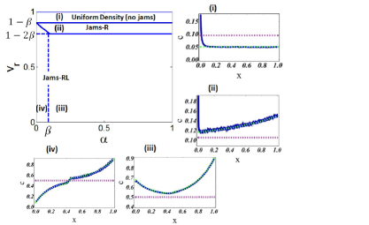
Figure 4: (Color online) Phase diagram in $\left(\alpha,v_{r}\right)$ space and typical density profiles, using $\beta=0.1$. $v_{r}>1-\beta$: Uniform density phase (no jams), with density profile (i). $1-\beta>v_{r}>1-\beta-c_{-}$: Jams-R phase where the behavior is dominated by the right boundary alone (density profile (ii)). $1-\beta-c_{-}>v_{r}$: Jams-LR phase where the behavior is influenced by both boundaries. The dashed vertical line separates this phase into two region: (iii) $\alpha>\beta$ and (iv) $\alpha<\beta$. Density profiles: Blue curves - simulation results; Green dashed curves - theoretical result of Eq.2; Horizontal dashed purple curves - bulk density $c_{b}$.

We find four regions of different average concentrations (Fig.3b, for more details see SI , Figs.S3,S4): (i) HD region near the tip, with density $1-v_{r}$, (ii) jammed regions of density $1$, (iii) free flow regions with density $\beta$, and (iv) the entrance region near the base with density $c_{-}=\min(\alpha,\frac{1-v_{r}}{2})$. The lines separating these different regions have slopes that can be calculated according to the shock velocities Kolomeisky et al. (1998); SI . Using these slopes, we can find the meeting points between the different regions within the space-time slice. This allows us to calculate the time-duration that each spatial point spends in a region of certain density.

One such important triple meeting point is between the regions of densities $[1-v_{r},\beta,c_{-}]$, which if it exists defines the meeting between the regions influenced by both boundaries (Fig.3). If it does not exist as a real meeting point, it nevertheless defines the location of the matching between the left and right solutions. The location of this point is given by

$$x_{w}=\frac{v_{r}(1-v_{r}-\beta-c_{-})}{v_{r}(1-v_{r}-\beta-c_{-})+\beta(1-c_{-})}$$ (1)

Summing the contributions of each region, we get that the average density profile is given by

$$x>x_{w}:$$

$$c(x) =\frac{\beta}{\beta+v_{r}}+\left(1-v_{r}-\frac{\beta}{\beta+v_{r}}\right)\exp{\left(\frac{x-1}{\xi_{r}}\right)}$$

$$x<x_{w}:$$

$$c(x) =\frac{\beta}{\beta+v_{r}}+\frac{v_{r}\left(c_{-}-\beta\right)}{(c_{-}+v_{r})(\beta+v_{r})}\exp{\left(-\frac{x}{\xi_{l}}\right)}$$

$$+\left(1-c_{-}-\frac{c_{-}}{c_{-}+v_{r}}\right)\cdot\exp{\left(\frac{\Lambda_{f}(1-v_{r})(c_{-}-\beta)}{c_{-}\beta}(x_{w}-1)\right)}\cdot$$

$$\exp{\left(\frac{\Lambda_{f}(1-v_{r})(1-c_{-})}{c_{-}}(x-1)\right)}$$ (2)

where

$$\xi_{r}=\frac{\beta}{\Lambda_{f}(1-\beta)(1-v_{r})},\xi_{l}=\frac{v_{r}(1-v_{r}-\beta-c_{-})}{\Lambda_{f}(1-c_{-})(1-vr)(1-\beta)}$$ (3)

$\xi_{l},\xi_{r}$ are the ’healing’ lengths of the left and right exponentials respectively as shown in Fig. 4(i)-(iii). The agreement between the simulations and the calculated density profile (Eq.2) is very good, and improves for large systems $L\rightarrow\infty$. For comparison, we also denote the bulk density predicted from the periodic model Mallick (1996) with retrograde flow: $c_{b}=\beta/(\beta+v_{r})$ SI , as seen in Eq.2.

The jam size in the bulk is an exponential random variable with mean value

$$\left\langle\Omega\right\rangle=L\frac{\beta}{\Lambda_{f}}\frac{1-v_{r}-\beta}{(1-v_{r})(1-\beta)}$$ (4)

We compare this result with simulation in Fig. S5 in SI and we see that the two agree very well.

The phase diagram of the system, is shown in Fig. 4. We first note that for $\beta=1-v_{r}$, both the mean jam size (Eq.4) and the exponential accumulation at the tip (Eq.2) vanishes. For $\beta>1-v_{r}$ we indeed find that the system does not exhibit any jams (except for the usual background of TASEP fluctuations), and the concentration is flat throughout the system at a value of $1-v_{r}$ (except for a shock at the left boundary, Fig.4i). The system behave as TASEP with retrograde flow $v_{r}$ and zero current. This second-order transition can also be understood in terms of the velocities of the holes entering the system at the tip SI . Note that in the limit $v_{r}=0$, inactive particles will get stuck in the first site, preventing new particles from entering the system. This can be fixed by changing the b.c., so that the inactive particle is also removed at the left boundary.

Next, we note that $x_{w}$ becomes negative when: $1-v_{r}-c_{-}<\beta$, which corresponds to a vanishing of the left exponential in $c(x)$, and therefore this phase is denoted as Jams-R (Fig.4, and profile (ii)). Finally for positive $x_{w}$ (denoted as Jams-LR phase in Fig.4) we find that: for $\alpha>\beta$ jams grow as they approach the base (near the left end, Fig.4iii), while for $\alpha<\beta$ they shrink (Fig.4iv). This means that for $\alpha<\beta$ there is a step-like profile, with the step located at $x_{w}$. The steepness of the step is given by the exponential localized at $x_{w}$ in eq. (2). Taking the limit of $\alpha\rightarrow 0$ by using the scaling $\alpha\sim 1/L$ and $L\rightarrow\infty$, results in the formation of a shock at $x_{w}$ (Fig. 5a). We find that the location of the shock in the system has a reentrant behavior as a function of $v_{r}$ (Fig. 5b), while the amplitude of the density discontinuity ($\Delta c$, Eq.S44) is also non-monotonic (Fig. 5c).

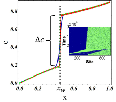
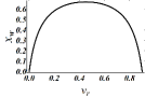
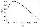
Figure 5: (Color online) System exhibiting a shock: Density profile for $\alpha=1/L,\beta=0.1,v_{r}=0.1,\Lambda_{f}=0.1$ with $L=10^{3}$ (blue curve) and $L=10^{4}$ (red curve). Green dashed line is the theoretical result of Eq. 2. Inset: Kymogrpah of the system. (b) The shock location $x_{w}$ from Eq.1 and, (c) the density jump at the shock ($\Delta c$, Eq.S44).

Unlike previous shocks found in TASEP-like models Parmeggiani et al. (2003); Reichenbach et al. (2006); Hinsch and Frey (2006); Arita et al. (2013) the shock we find is only defined for the average concentration, while it maintains a dynamic nature: it undergoes intermittent collapses (kymograph in Fig. 5). Furthermore, these shocks do not obey the usual Rankine-Hugoniot relation that follows from naive MFA: $c(x^{-}_{w})=1-c(x^{+}_{w})-v_{r}$. During the time that no motor is switched off at the tip, there is an accumulation of particles and a domain wall fulfilling the shock relation is established: $c(x^{-}_{w})=0,c(x^{+}_{w})=1-v_{r}$, so that: $\Delta c|_{x_{w}}=1-v_{r}$. The probability that such a domain wall exists at any given time is given in Eq.S47, and is simply the fraction of time duration that no jam is initiated at the tip.

Discussion. Our model is able to reproduce two experimental observations of molecular motors in actin-based cellular protrusions, namely the finite accumulation length of the motors at the protrusions’ tips, and the formation of backward-moving aggregates of motors from the tip to the base. In our model these phenomena are linked and both arise from the random process of traffic-jam initiation at the tip, followed by the ”relay-race”-like transport of the cargo between the motors. Note however, that this mechanism is maintaining individual motors near the tip, since only one motor is recycled back to the cytoplasm per traffic jam. Since there are multiple parallel actin tracks inside a real protrusion, we expect the turnover of motors to be more efficient than our one-dimensional model suggests. The effects of such parallel tracks, as well as those of attachment/detachment kinetics will be explored in a future elaboration of this work.

Since the cargo carried by the motors is often involved in enhancing the actin polymerization at the tip Tokuo and Ikebe (2004); Salles et al. (2009); Manor et al. (2011), a full treatment of this system should include a feedback between the system size and motor/cargo distribution during the growth phase and the fluctuations around the steady-state length. While in the current work we considered a fixed geometry, we propose to investigate the feedback between motors and protrusion length in the future, similar to Melbinger et al. (2012); Sugden et al. (2007); Sugden and Evans (2007).

From the theory point of view we introduce here a model that has several unique features, compared to previous models of molecular motors on cytoskeletal tracks Lipowsky et al. (2001); Johann et al. (2012); Melbinger et al. (2012); Sugden et al. (2007): (i) We find that the MFA fails, while it works well in separated domains of the system that are connected through shocks, (ii) we find that while there is a steady-state average density, the spatio-temporal behavior of the system is inherently dynamic exhibiting large fluctuations, (iii) a discontinuity (shock) can appear in the average steady-state density profile, but this shock is inherently dynamic and undergoes intermittent collapses.

Finally, we can make several qualitative predictions. Both the actin polymerization rate ($v_{r}$) and the influx of motors ($\alpha$) may be modified in experiments, and therefore the phase diagram of fig. 4 explored. We predict that increasing the retrograde flow will result in a decrease of the average jam size, as follows from eq. (4). The parameters $K_{f},\beta$ are controlled by the cargo affinity to the motors: By modifying $\beta$ the system will change its phase according to Fig. 4a, and through $K_{f}$ the average size of the jams can be manipulated (eq. 4).