Low-complexity 8-point DCT Approximations
Based on Integer Functions

Abstract

In this paper, we propose a collection of approximations for the 8-point discrete cosine transform (DCT) based on integer functions. Approximations could be systematically obtained and several existing approximations were identified as particular cases. Obtained approximations were compared with the DCT and assessed in the context of JPEG-like image compression.

1 Introduction

The discrete cosine transform (DCT) is widely regarded as a key operation in digital signal processing [51, 15]. In fact, the Karhunen-Loève transform (KLT) is the asymptotic equivalent of the DCT, being the former an optimal transform in terms of decorrelation and energy compaction properties [1, 18, 51, 15, 37, 23]. When high correlated first-order Markov signals are considered [51, 15]—such as natural images [37]— the DCT can closely emulate the KLT [1].

The DCT has been considered and effectively adopted in a number of methods for image and video coding [6]. In fact, the DCT is the central mathematical operation for the following standards: JPEG [58, 46], MPEG-1 [52], MPEG-2 [28], H.261 [30], H.263 [31], H.264 [61, 33, 40, 61], and the recent HEVC [49, 8, 54]. In all above standards, the particular 8-point DCT is considered.

Thus, developing fast algorithms for the efficient evaluation of the 8-point DCT is a main task in the circuits, systems, and signal processing communities. Archived literature contains a multitude of fast algorithms for this particular blocklength [57, 26]. Remarkably extensive reports have been generated amalgamating scattered results for the 8-point DCT [51, 15]. Among the most popular techniques, we mention the following algorithms: Wang factorization [59], Lee DCT for power-of-two blocklengths [35], Arai DCT scheme [2], Loeffler algorithm [39], Vetterli-Nussbaumer algorithm [57], Hou algorithm [26], and Feig-Winograd factorization [20]. All these methods are classical results in the field and have been considered for practical applications [52, 56, 38]. For instance, the Arai DCT scheme was employed in various recent hardware implementations of the DCT [42, 50, 19].

Naturally, DCT fast algorithms that result in major computational savings compared to direct computation of the DCT were already developed decades ago. In fact, the intense research in the field has led to methods that are very close to the theoretical complexity of DCT [37, 41, 24, 39, 2]. Thus, the computation of the exact DCT is a task with very little room for major improvements in terms of minimization of computational complexity by means of standard methods.

On the other hand, DCT approximations—operations that closely emulate the DCT— are mathematical tools that can furnish an alternative venue for DCT evaluation. Effectively, DCT approximations have already been considered in a number of works [15, 23, 4, 10, 13]. Moreover, although usual fast algorithms can reduce the computational complexity significantly, they still need floating-point operations [15]. In contrast, approximate DCT methods can be tailored to require very low arithmetic complexity.

A comprehensive list of approximate methods for the DCT is found in [15]. Prominent techniques include the signed DCT (SDCT) [23], the binDCT [37], the level 1 approximation by Lengwehasatit-Ortega [36], the Bouguezel-Ahmad-Swamy (BAS) series of algorithms [9, 10, 11, 12, 13, 14], the DCT round-off approximation [17], the modified DCT round-off approximation [4], and the multiplier-free DCT approximation for RF imaging [48].

The goal of this paper is two-fold. First, we aim at proposing a systematic procedure for deriving low-complexity approximations for the 8-point DCT. For such, we consider several types of rounding-off functions applied to scaled the exact 8-point DCT matrix. The entries of the sough approximate DCT matrices are required to possess null multiplicative complexity; only additions and simple bit-shifting operations are allowed. Second, we focus on suggesting practical approximations and assessing them as tools for JPEG-like image compression.

The paper unfolds as follows. In Section 2, we describe the mathematical framework of the DCT and we discuss the polar decomposition method for DCT approximation [16]. In Section 3, we propose a systematic method based on integer functions for obtaining low-complexity matrices useful for generating DCT approximations. The discussed method is based on a computational search over a subset of candidate matrices under constraints of low-computational complexity and orthogonality or near orthogonality. In Section 4, we provide details of the computational search and list the obtained approximations. Section LABEL:sec:Fast_Algorithm presents fast algorithms for the obtained approximations. In Section 6, the resulting approximations are subject to performance assessment in the context of image compression using image quality measures as figures of merit. In Section 7, we state concluding remarks.

2 Exact and Approximate DCT

2.1 Mathematical Preliminaries

The $N$-point DCT is algebraically represented by the $N\times N$ transformation matrix $\mathbf{C}_{N}$ whose elements are given by [51, 15]

$$c_{m,n}=\frac{1}{\sqrt{N}}\,\beta_{m-1}\cos\left(\frac{\pi(m-1)(2n-1)}{2N}\right),$$

where $m,n=1,2,\ldots,N$, $\beta_{0}=1$, and $\beta_{k}=\sqrt{2}$, for $k\neq 0$. Let $\mathbf{x}=\begin{bmatrix}x_{0}&x_{1}&\cdots&x_{N-1}\end{bmatrix}^{\top}$ be an input vector, where the superscript ^⊤ denotes the transposition operation. The one-dimensional (1-D) DCT transform of $\mathbf{x}$ is the $N$-point vector $\mathbf{X}=\begin{bmatrix}X_{0}&X_{1}&\cdots&X_{N-1}\end{bmatrix}^{\top}$ given by $\mathbf{X}=\mathbf{C}_{N}\cdot\mathbf{x}$. Because $\mathbf{C}_{N}$ is an orthogonal matrix, the inverse transformation can be written according to $\mathbf{x}=\mathbf{C}_{N}^{\top}\cdot\mathbf{X}$.

Let $\mathbf{A}$ and $\mathbf{B}$ be square matrices of size $N$. For two-dimensional (2-D) signals, we have the following expressions that relate the forward and inverse 2-D DCT operations, respectively:

$$\mathbf{B}=\mathbf{C}_{N}\cdot\mathbf{A}\cdot\mathbf{C}_{N}^{\top}\quad\text{and}\quad\mathbf{A}=\mathbf{C}_{N}^{\top}\cdot\mathbf{B}\cdot\mathbf{C}_{N}.$$ (1)

Although the procedures described in this work can be applied to any blocklength, we focus exclusively on the 8-point DCT. Thus, for simplicity, the 8-point DCT matrix is denoted as $\mathbf{C}$ and is given by:

$$\mathbf{C}\triangleq\mathbf{C}_{8}=\frac{1}{2}\cdot\begin{bmatrix}\hbox{}\,\vbox{\Let@\restore@math@cr\default@tag\halign{\hfil$\m@th\scriptstyle#$&&\thickspace\hfil$\m@th\scriptstyle#$\cr\gamma_{3}&\gamma_{3}&\gamma_{3}&\gamma_{3}&\gamma_{3}&\gamma_{3}&\gamma_{3}&\gamma_{3}\\ \gamma_{0}&\gamma_{2}&\gamma_{4}&\gamma_{6}&-\gamma_{6}&-\gamma_{4}&-\gamma_{2}&-\gamma_{0}\\ \gamma_{1}&\gamma_{5}&-\gamma_{5}&-\gamma_{1}&-\gamma_{1}&-\gamma_{5}&\gamma_{5}&\gamma_{1}\\ \gamma_{2}&-\gamma_{6}&-\gamma_{0}&-\gamma_{4}&\gamma_{4}&\gamma_{0}&\gamma_{6}&-\gamma_{2}\\ \gamma_{3}&-\gamma_{3}&-\gamma_{3}&\gamma_{3}&\gamma_{3}&-\gamma_{3}&-\gamma_{3}&\gamma_{3}\\ \gamma_{4}&-\gamma_{0}&\gamma_{6}&\gamma_{2}&-\gamma_{2}&-\gamma_{6}&\gamma_{0}&-\gamma_{4}\\ \gamma_{5}&-\gamma_{1}&\gamma_{1}&-\gamma_{5}&-\gamma_{5}&\gamma_{1}&-\gamma_{1}&\gamma_{5}\\ \gamma_{6}&-\gamma_{4}&\gamma_{2}&-\gamma_{0}&\gamma_{0}&-\gamma_{2}&\gamma_{4}&-\gamma_{6}\crcr}}\,\end{bmatrix},$$

where $\gamma_{k}=\cos(2\pi(k+1)/32)$, $k=0,1,\ldots,6$. These quantities are algebraic integers explicitly given by [42]:

$$\gamma_{0} =\frac{\sqrt{2+\sqrt{2+\sqrt{2}}}}{2}\approx 0.9808\ldots,\qquad\gamma_{1}=\frac{\sqrt{2+\sqrt{2}}}{2}\approx 0.9239\ldots,$$

$$\gamma_{2} =\frac{\sqrt{2+\sqrt{2-\sqrt{2}}}}{2}\approx 0.8315\ldots,\qquad\gamma_{3}=\frac{\sqrt{2}}{2}\approx 0.7071\ldots,$$

$$\gamma_{4} =\frac{\sqrt{2-\sqrt{2-\sqrt{2}}}}{2}\approx 0.5556\ldots,\qquad\gamma_{5}=\frac{\sqrt{2-\sqrt{2}}}{2}\approx 0.3827\ldots,$$

$$\gamma_{6} =\frac{\sqrt{2-\sqrt{2+\sqrt{2}}}}{2}\approx 0.1951\ldots$$

In this work, we adopt the following terminology. A matrix $\mathbf{A}$ is orthogonal if $\mathbf{A}\cdot\mathbf{A}^{\top}$ is a diagonal matrix. In particular, if $\mathbf{A}\cdot\mathbf{A}^{\top}$ is the identity matrix, then $\mathbf{A}$ is said to be orthonormal.

2.2 DCT Approximations

Generally, a DCT approximation is a transformation $\hat{\mathbf{C}}$ that—according to some specified metric— behaves similarly to the exact DCT matrix $\mathbf{C}$. An approximation matrix $\hat{\mathbf{C}}$ is usually based on a transformation matrix $\mathbf{T}$ of low computational complexity. Indeed, matrix $\mathbf{T}$ is the key component of a given DCT approximation.

Often the elements of the transformation matrix $\mathbf{T}$ possess null multiplicative complexity. For instance, this property can be satisfied by restricting the entries of $\mathbf{T}$ to the set of powers of two $\{0,\pm 1,\pm 2,\pm 4,\pm 8,\ldots\}$. In fact, multiplications by such elements are trivial and require only bit-shifting operations.

Approximations for the DCT can be classified into two categories depending on whether $\hat{\mathbf{C}}$ is orthonormal or not. In principle, given a low-complexity matrix $\mathbf{T}$ it is possible to derive an orthonormal matrix $\hat{\mathbf{C}}$ based on $\mathbf{T}$ by means of the polar decomposition [16, 53]. Indeed, if $\mathbf{T}$ is a full rank real matrix, then the following factorization is uniquely determined:

$$\hat{\mathbf{C}}=\mathbf{S}\cdot\mathbf{T},$$ (2)

where $\mathbf{S}$ is a symmetric positive definite matrix [53, p. 348]. Matrix $\mathbf{S}$ is explicitly related to $\mathbf{T}$ according to the following relation:

$$\mathbf{S}=\sqrt{(\mathbf{T}\cdot\mathbf{T}^{\top})^{-1}},$$

where $\sqrt{\cdot}$ denotes the matrix square root operation [25, 43]. Being orthonormal, such type of approximation satisfies $\hat{\mathbf{C}}^{-1}=\hat{\mathbf{C}}^{\top}$. Therefore, we have that

$$\hat{\mathbf{C}}^{-1}=\mathbf{T}^{\top}\cdot\mathbf{S}.$$

As a consequence, the inverse transformation $\hat{\mathbf{C}}^{-1}$ inherits the same computational complexity of the forward transformation.

From the computational point of view, it is desirable that $\mathbf{S}$ be a diagonal matrix. In this case, the computational complexity of $\hat{\mathbf{C}}$ is the same as that of $\mathbf{T}$, except for the scale factors in the diagonal matrix $\mathbf{S}$. Moreover, depending on the considered application, even the constants in $\mathbf{S}$ can be disregarded in terms of computational complexity assessment. This occurs when the involved constants are trivial multiplicands, such as the powers of two. Another more practical possibility for neglecting the complexity of $\mathbf{S}$ arises when it can be absorbed into other sections of a larger procedure. This is the case in JPEG-like compression, where the quantization step is present [58]. Thus, matrix $\mathbf{S}$ can be incorporated into the quantization matrix [4, 13, 36, 9, 11, 17, 5]. In terms of the inverse transformation, it is also beneficial that $\mathbf{S}$ is diagonal, because the complexity of $\hat{\mathbf{C}}^{-1}$ becomes essentially that of $\mathbf{T}^{\top}$.

In order that $\mathbf{S}$ be a diagonal matrix, it is sufficient that $\mathbf{T}$ satisfies the orthogonality condition:

$$\mathbf{T}\cdot\mathbf{T}^{\top}=\mathbf{D},$$ (3)

where $\mathbf{D}$ is a diagonal matrix [16].

If (3) is not satisfied, then $\mathbf{S}$ is not a diagonal and the advantageous properties of the resulting DCT approximation are in principle lost. In this case, the off-diagonal elements contribute to a computational complexity increase and the absorption of matrix $\mathbf{S}$ cannot be easily done. However, at the expense of not providing an orthogonal approximation, one may consider approximating $\mathbf{S}$ itself by replacing the off-diagonal elements of $\mathbf{D}$ by zeros. Thus, the resulting matrix $\hat{\mathbf{S}}$ is given by:

$$\hat{\mathbf{S}}=\sqrt{[\operatorname{diag}(\mathbf{T}\cdot\mathbf{T}^{\top})]^{-1}},$$

where $\operatorname{diag}(\cdot)$ returns a diagonal matrix with the diagonal elements of its matrix argument. Thus, the non-orthogonal approximation is furnished by:

$$\tilde{\mathbf{C}}=\hat{\mathbf{S}}\cdot\mathbf{T}.$$

Matrix $\tilde{\mathbf{C}}$ can be a meaningful approximation if $\hat{\mathbf{S}}$ is, in some sense, close to $\mathbf{S}$; or, alternatively, if $\mathbf{T}$ is almost orthogonal.

From the algorithm designing perspective, proposing non-orthogonal approximations may be a less demanding task, since (3) is not required to be satisfied. However, since $\tilde{\mathbf{C}}$ is not orthogonal, the inverse transformation must be cautiously examined. Indeed, the inverse transformation does not employ directly the low-complexity matrix $\mathbf{T}$ and is given by

$$\tilde{\mathbf{C}}^{-1}=\mathbf{T}^{-1}\cdot\hat{\mathbf{S}}^{-1}.$$

Even if $\mathbf{T}$ is a low-complexity matrix, it is not guaranteed that $\mathbf{T}^{-1}$ also possesses low computational complexity figures. Nevertheless, it is possible to obtain non-orthogonal approximations whose both direct and inverse transformation matrices have low computational complexity. Two prominent examples are the SDCT [23] and the BAS approximation described in [9].

3 Scaling and Integer Mapping

Approximations archived in literature often possess transformation matrices with entries defined on the set $\mathcal{C}_{0}=\{0,\pm 1,\pm 2\}$ [4, 17, 23, 13, 14]. Thus such transformations possess null multiplicative complexity, because the required arithmetic operations can be implemented exclusively by means of additions and bit-shifting operations. However, in [32, 44], an image compression scheme based on the Tchebichef transform was advanced for image compression. This particular method employs a discrete transfromation referred to as the discrete Tchebichef transform (DTT) [32]. The implied DTT matrix possesses entries defined on $\mathcal{C}_{0}$ but also considers the elements $\pm 3$. Multiplications by constants $\pm 3$ can be implemented by means of one addition and one bit-shifting operation ($3\cdot x=2\cdot x+x$). Thus, as suggested in [32], in this work, we adopt $\mathcal{C}=\mathcal{C}_{0}\cup\{\pm 3\}$ as the domain set of the entries for the sought DCT approximations. Nevertheless, we emphasize that approximations with entries $\pm 3$ are expected to possess a higher computational complexity.

In [23] Haweel introduced a simple approach for designing a DCT approximation. The DCT approximation termed SDCT was defined as follows [23]:

$$\operatorname{sign}(\mathbf{C}),$$

where $\operatorname{sign}(\cdot)$ is the signum function is applied to each entry of $\mathbf{C}$ and is given by

$$\operatorname{sign}(x)=\begin{cases}+1,&\text{if $x>0$},\\ 0,&\text{if $x=0$},\\ -1,&\text{if $x<0$}.\end{cases}$$

The SDCT can be regarded as a seminal work in the field of DCT approximations.

Additionally, in [16, 17, 3] a low-complexity DCT approximation was proposed based on the following matrix:

$$\operatorname{round}(2\cdot\mathbf{C}),$$

where $\operatorname{round}(\cdot)$ is the entrywise rounding-off function as implemented in Matlab. In this work, we aim at expanding and generalizing these approximations.

As a venue to design DCT approximations, we consider integer functions [22, Cap. 3]. An integer function is simply a function whose values are integers. We aim at mapping the exact entries of the DCT matrix into integer quantities. The resulting matrix is sought to approximate the DCT. For such end, we adopt the following general mapping:

$$\begin{split}\mathbb{R}&\longrightarrow\mathcal{M}_{8}(\mathbb{Z})\\ \alpha&\longmapsto\operatorname{int}\left(\alpha\cdot\mathbf{C}\right),\end{split}$$ (4)

where $\mathcal{M}_{8}(\mathbb{Z})$ is the space of 8$\times$8 matrices over the set of integers $\mathbb{Z}$, $\operatorname{int}(\cdot)$ is a prototype integer function [22, p. 67]. Function $\operatorname{int}(\cdot)$ operates entrywise over its matrix argument. Parameter $\alpha$ is termed the expansion factor and scales the exact DCT matrix allowing a wide range of possible integer mappings [47].

Particular examples of integer functions are the floor, the ceiling, the truncation (round towards zero), and the round-away-from-zero function. These functions are defined, respectively, as follows:

$$\operatorname{floor}(x) =\lfloor x\rfloor=\max\,\{m\in\mathbb{Z}\mid m\leq x\},$$

$$\operatorname{ceil}(x) =\lceil x\rceil=\min\,\{n\in\mathbb{Z}\mid n\geq x\},$$

$$\operatorname{trunc}(x) =\operatorname{sign}(x)\cdot\left\lfloor\left|x\right|\right\rfloor,$$

$$\operatorname{round}_{\text{AFZ}}(x) =\operatorname{sign}(x)\cdot\left\lceil\left|x\right|\right\rceil,$$

where $|\cdot|$ returns the absolute value of its argument.

Another particularly useful integer function is the round to nearest integer function [45, p. 73]. This function possesses various definitions depending on its behavior for input arguments whose fractional part is exactly $1/2$. Thus, we have the following rounding-off functions: round-half-up, round-half-down, round-half-away-from-zero, round-half-towards-zero, round-half-to-even, and round-half-to-odd function. These different nearest integer functions are, respectively, given by:

$$\operatorname{round}_{\text{HU}}(x) =\left\lfloor x+\frac{1}{2}\right\rfloor,$$

$$\operatorname{round}_{\text{HD}}(x) =\left\lceil x-\frac{1}{2}\right\rceil,$$

$$\operatorname{round}_{\text{HAFZ}}(x) =\operatorname{sign}(x)\cdot\left\lfloor\left|x\right|+\frac{1}{2}\right\rfloor,$$

$$\operatorname{round}_{\text{HTZ}}(x) =\operatorname{sign}(x)\cdot\left\lceil\left|x\right|-\frac{1}{2}\right\rceil,$$

$$\operatorname{round}_{\text{EVEN}}(x) =\begin{cases}\left\lfloor x-\frac{1}{2}\right\rfloor,&\text{if $\frac{2x-1}{4}\in\mathbb{Z}$,}\\ \left\lfloor x+\frac{1}{2}\right\rfloor,&\text{otherwise,}\\ \end{cases}$$

$$\operatorname{round}_{\text{ODD}}(x) =\begin{cases}\left\lfloor x+\frac{1}{2}\right\rfloor,&\text{if $\frac{2x-1}{4}\in\mathbb{Z}$,}\\ \left\lfloor x-\frac{1}{2}\right\rfloor,&\text{otherwise.}\\ \end{cases}$$

The round-half-away-from-zero function is the implementation employed in the round function in Matlab/Octave. The international technical standard ISO/IEC/IEEE 60559:2011 recommends $\operatorname{round}_{\text{EVEN}}(\cdot)$ as the nearest integer function of choice [29]. This latter implementation is adopted in the scientific computation software Mathematica [62].

4 Computational Search

4.1 Problem Setup

In this section, we exhaustively compute (4) for judiciously chosen values of $\alpha$ such that the following conditions about $\mathbf{T}=\operatorname{int}(\alpha\cdot\mathbf{C})$ are satisfied:

1. matrix $\mathbf{T}$ must possess its elements defined on $\mathcal{C}$;

2. $\mathbf{T}\cdot\mathbf{T}^{\top}$ must be a diagonal matrix or must exhibit a small deviation from diagonality in the sense described in [21];

3. if $\mathbf{T}$ is not orthogonal (cf. (3)), but $\mathbf{T}\cdot\mathbf{T}^{\top}$ is approximately a diagonal matrix, then the inverse matrix $\mathbf{T}^{-1}$ must possess low-complexity with its elements defined on $\mathcal{C}$.

Condition (a) ensures that the forward transformation is a low-complexity operation. Therefore, in terms of implementation, it may require simple hardware structures. If (3) is satisfied, then the inverse transformation is guaranteed to have low computation complexity. This is because $\mathbf{T}$ becomes the transpose of itself, apart from the multiplication by a diagonal matrix. On the other hand, if (3) is not satisfied, then resulting matrices may not be useful in contexts that depend on orthogonalization. Nevertheless, if $\mathbf{T}\cdot\mathbf{T}^{\top}$ is ‘almost’ diagonal, then $\mathbf{T}$ can be of interest. In that case, one may explicitly check whether $\mathbf{T}^{-1}$ has low complexity. Thus, Condition (c) is considered.

To quantify the deviation from diagonality, as required in Condition (b), we adopt the following measure, called deviation from diagonality.

Definition 1

Let $\mathbf{A}$ be a square matrix. Then its deviation from diagonality is given by [21]:

$$\operatorname{\delta}(\mathbf{A})=1-\frac{\|\operatorname{diag}(\mathbf{A})\|_{\text{F}}}{\|\mathbf{A}\|_{\text{F}}},$$

where $\|\cdot\|_{\text{F}}$ denotes the Frobenius norm for matrices [53].

As a decision criterion, we adopt the deviation from diagonality exhibited by the SDCT as the maximum deviation acceptable for non-orthogonal approximations. The SDCT was chosen as a reference transformation because (i) it has proven good properties [23] and (ii) it is widely employed in performance comparisons [17, 4, 10, 9, 11, 12, 14]. Thus, according to this criterion, Condition (b) becomes:

1. $\operatorname{\delta}\left(\mathbf{T}\cdot\mathbf{T}^{\top}\right)\leq 1-\frac{2}{\sqrt{5}}\approx 0.1056$.

In order that the entries of $\operatorname{int}(\alpha\cdot\mathbf{C})$ are defined on $\mathcal{C}$, we must restrict the range of $\alpha$. We notice that the largest element of $\mathbf{C}$ is $\gamma_{0}/2$. Thus, it is sufficient to solve the following inequality for $\alpha$: $0\leq\operatorname{int}(\alpha\cdot\gamma_{0}/2)\leq 3$. For the ceiling, floor, truncation, round-away-from-zero, and all nearest integer functions, respectively, we have the following ranges of $\alpha$: $\left[0,\frac{6}{\gamma_{0}}\right]$, $\left[\frac{2}{\gamma_{0}},\frac{8}{\gamma_{0}}\right]$, $\left[\frac{2}{\gamma_{0}},\frac{8}{\gamma_{0}}\right]$, $\left[0,\frac{6}{\gamma_{0}}\right]$, and $\left[\frac{1}{\gamma_{0}},\frac{7}{\gamma_{0}}\right]$.

4.2 Obtained Approximations

In terms of Condition (a), the ceiling function could supply only one low-complexity non-orthogonal candidate matrix for DCT approximation as shown in Table 1. However, its deviation from diagonality is exceedingly high. In fact, we have that $\operatorname{\delta}(\tilde{\mathbf{T}}_{0})\approx 0.4548$. For such reason, this particular approximation will not be further considered in this paper. Hereafter, we only list matrices that satisfy all prescribed conditions.

The floor function could not furnish any matrix under the prescribed requirements. On the other hand, when considering the truncation function, five matrices were obtained, being listed in Table 2. Both orthogonal and non-orthogonal matrices were found. Similarly, for the round-away-from-zero function, a set of four distinct matrices was derived. These matrices are shown in Table 3. We notice that matrices $\mathbf{T}_{4}$ and $\tilde{\mathbf{T}}_{2}$ coincide with the rounded DCT reported in [17] and the SDCT [23], respectively. Moreover, we have that

$$\tilde{\mathbf{T}}_{4}=\left[\begin{smallmatrix}2&0&0&0&0&0&0&0\\ 0&1&0&0&0&0&0&0\\ 0&0&1&0&0&0&0&0\\ 0&0&0&1&0&0&0&0\\ 0&0&0&0&2&0&0&0\\ 0&0&0&0&0&1&0&0\\ 0&0&0&0&0&0&1&0\\ 0&0&0&0&0&0&0&1\\ \end{smallmatrix}\right]\cdot\tilde{\mathbf{T}}_{3}.$$ (5)

As a consequence, by means of (2), both $\tilde{\mathbf{T}}_{3}$ and $\tilde{\mathbf{T}}_{4}$ lead to the same DCT approximation.

Table 1: Ceiling function

Approximation	Transformation Matrix	Range of $\alpha$	Orthogonal?
$\tilde{\mathbf{T}}_{0}$	$\left[\hbox{}\,\vbox{\Let@\restore@math@cr\default@tag\halign{\hfil$\m@th\scriptstyle#$&&\thickspace\hfil$\m@th\scriptstyle#$\cr 1&1&1&1&1&1&1&1\\ 1&1&1&1&0&0&0&0\\ 1&1&0&0&0&0&1&1\\ 1&0&0&0&1&1&1&0\\ 1&0&0&1&1&0&0&1\\ 1&0&1&1&0&0&1&0\\ 1&0&1&0&0&1&0&1\\ 1&0&1&0&1&0&1&0\\ }}\,\right]$	$(0,2/\gamma_{4})$	No

Table 2: Truncation function

Approximation	Transformation Matrix	Range of $\alpha$	Orthogonal?
$\mathbf{T}_{0}$	$\left[\hbox{}\,\vbox{\Let@\restore@math@cr\default@tag\halign{\hfil$\m@th\scriptstyle#$&&\thickspace\hfil$\m@th\scriptstyle#$\cr 1&1&1&1&1&1&1&1\\ 1&1&1&0&0&-1&-1&-1\\ 1&0&0&-1&-1&0&0&1\\ 1&0&-1&-1&1&1&0&-1\\ 1&-1&-1&1&1&-1&-1&1\\ 1&-1&0&1&-1&0&1&-1\\ 0&-1&1&0&0&1&-1&0\\ 0&-1&1&-1&1&-1&1&0\crcr}}\,\right]$	$(2/\gamma_{4},4/\gamma_{0})$	Yes
$\mathbf{T}_{1}$	$\left[\hbox{}\,\vbox{\Let@\restore@math@cr\default@tag\halign{\hfil$\m@th\scriptstyle#$&&\thickspace\hfil$\m@th\scriptstyle#$\cr 1&1&1&1&1&1&1&1\\ 2&1&1&0&0&-1&-1&-2\\ 0&1&-1&0&0&-1&1&0\\ 1&0&-2&-1&1&2&0&-1\\ 1&-1&-1&1&1&-1&-1&1\\ 1&-2&0&1&-1&0&2&-1\\ 1&0&0&-1&-1&0&0&1\\ 0&-1&1&-2&2&-1&1&0\crcr}}\,\right]$	$(4/\gamma_{0},4/\gamma_{1})$	Yes
$\mathbf{T}_{2}$	$\left[\hbox{}\,\vbox{\Let@\restore@math@cr\default@tag\halign{\hfil$\m@th\scriptstyle#$&&\thickspace\hfil$\m@th\scriptstyle#$\cr 1&1&1&1&1&1&1&1\\ 2&1&1&0&0&-1&-1&-2\\ 2&0&0&-2&-2&0&0&2\\ 1&0&-2&-1&1&2&0&-1\\ 1&-1&-1&1&1&-1&-1&1\\ 1&-2&0&1&-1&0&2&-1\\ 0&-2&2&0&0&2&-2&0\\ 0&-1&1&-2&2&-1&1&0\\ }}\,\right]$	$(4/\gamma_{1},4/\gamma_{2})$	Yes
$\mathbf{T}_{3}$	$\left[\hbox{}\,\vbox{\Let@\restore@math@cr\default@tag\halign{\hfil$\m@th\scriptstyle#$&&\thickspace\hfil$\m@th\scriptstyle#$\cr 2&2&2&2&2&2&2&2\\ 3&2&2&0&0&-2&-2&-3\\ 3&1&-1&-3&-3&-1&1&3\\ 2&0&-3&-2&2&3&0&-2\\ 2&-2&-2&2&2&-2&-2&2\\ 2&-3&0&2&-2&0&3&-2\\ 1&-3&3&-1&-1&3&-3&1\\ 0&-2&2&-3&3&-2&2&0\\ }}\,\right]$	$(4/\gamma_{4},6/\gamma_{2})$	Yes
$\tilde{\mathbf{T}}_{1}$	$\left[\hbox{}\,\vbox{\Let@\restore@math@cr\default@tag\halign{\hfil$\m@th\scriptstyle#$&&\thickspace\hfil$\m@th\scriptstyle#$\cr 1&1&1&1&1&1&1&1\\ 1&1&0&0&0&0&-1&-1\\ 1&0&0&-1&-1&0&0&1\\ 1&0&-1&0&0&1&0&-1\\ 1&-1&-1&1&1&-1&-1&1\\ 0&-1&0&1&-1&0&1&0\\ 0&-1&1&0&0&1&-1&0\\ 0&0&1&-1&1&-1&0&0\\ }}\,\right]$	$(2/\gamma_{3},2/\gamma_{4})$	No

Table 3: Round-away-from-zero function

Approximation	Transformation Matrix	Range of $\alpha$	Orthogonal?
$\mathbf{T}_{4}$ [17]	$\left[\hbox{}\,\vbox{\Let@\restore@math@cr\default@tag\halign{\hfil$\m@th\scriptstyle#$&&\thickspace\hfil$\m@th\scriptstyle#$\cr 1&1&1&1&1&1&1&1\\ 1&1&1&0&0&-1&-1&-1\\ 1&1&-1&-1&-1&-1&1&1\\ 1&0&-1&-1&1&1&0&-1\\ 1&-1&-1&1&1&-1&-1&1\\ 1&-1&0&1&-1&0&1&-1\\ 1&-1&1&-1&-1&1&-1&1\\ 0&-1&1&-1&1&-1&1&0\\ }}\,\right]$	$1/\gamma_{0}$	Yes
$\tilde{\mathbf{T}}_{2}$ [23]	$\left[\hbox{}\,\vbox{\Let@\restore@math@cr\default@tag\halign{\hfil$\m@th\scriptstyle#$&&\thickspace\hfil$\m@th\scriptstyle#$\cr 1&1&1&1&1&1&1&1\\ 1&1&1&1&-1&-1&-1&-1\\ 1&1&-1&-1&-1&-1&1&1\\ 1&-1&-1&-1&1&1&1&-1\\ 1&-1&-1&1&1&-1&-1&1\\ 1&-1&1&1&-1&-1&1&-1\\ 1&-1&1&-1&-1&1&-1&1\\ 1&-1&1&-1&1&-1&1&-1\\ }}\,\right]$	$(0,2/\gamma_{0})$	No
$\tilde{\mathbf{T}}_{3}$	$\left[\hbox{}\,\vbox{\Let@\restore@math@cr\default@tag\halign{\hfil$\m@th\scriptstyle#$&&\thickspace\hfil$\m@th\scriptstyle#$\cr 1&1&1&1&1&1&1&1\\ 2&2&1&1&-1&-1&-2&-2\\ 2&1&-1&-2&-2&-1&1&2\\ 2&-1&-2&-1&1&2&1&-2\\ 1&-1&-1&1&1&-1&-1&1\\ 1&-2&1&2&-2&-1&2&-1\\ 1&-2&2&-1&-1&2&-2&1\\ 1&-1&2&-2&2&-2&1&-1\\ }}\,\right]$	$(2/\gamma_{2},2/\gamma_{3}]$	No
$\tilde{\mathbf{T}}_{4}$	$\left[\hbox{}\,\vbox{\Let@\restore@math@cr\default@tag\halign{\hfil$\m@th\scriptstyle#$&&\thickspace\hfil$\m@th\scriptstyle#$\cr 2&2&2&2&2&2&2&2\\ 2&2&1&1&-1&-1&-2&-2\\ 2&1&-1&-2&-2&-1&1&2\\ 2&-1&-2&-1&1&2&1&-2\\ 2&-2&-2&2&2&-2&-2&2\\ 1&-2&1&2&-2&-1&2&-1\\ 1&-2&2&-1&-1&2&-2&1\\ 1&-1&2&-2&2&-2&1&-1\\ }}\,\right]$	$(2/\gamma_{3},2/\gamma_{4})$	No

The nearest integer function may result in different approximations when the choice of $\alpha$ results in a matrix $\alpha\cdot\mathbf{C}$ whose entries are possibly half-integers. The values of $\alpha$ that effect half-integers are of the form $l/\gamma_{k}$, $k=0,1,\ldots,6$, where $l\in\mathbb{Z}$. Apart from these critical points, the different types of nearest integer functions behave identically. By examining these boundary cases, we could establish intervals for which each of discussed nearest integer functions results in meaningful DCT approximations.

Table 4 brings the obtained low-complexity matrices derived from the round-half-up and round-half-down functions. Among the resulting matrices, we identify $\mathbf{T}_{6}$ as the approximation described in [48]. The remaining nearest integer functions supply no matrix different from the above listed ones. In Table 5, we show the resulting matrices.

Table 4: Round-half-up and round-half-down functions

Approximation	Transformation Matrix	Range of $\alpha$	Orthogonal?
$\mathbf{T}_{0}$	See Table 2	$(1/\gamma_{4},1/\gamma_{5})$	Yes
$\mathbf{T}_{4}$ [17]	See Table 3	$(1/\gamma_{5},3/\gamma_{0})$	Yes
$\mathbf{T}_{5}$	$\left[\hbox{}\,\vbox{\Let@\restore@math@cr\default@tag\halign{\hfil$\m@th\scriptstyle#$&&\thickspace\hfil$\m@th\scriptstyle#$\cr 1&1&1&1&1&1&1&1\\ 2&1&1&0&0&-1&-1&-2\\ 1&1&-1&-1&-1&-1&1&1\\ 1&0&-2&-1&1&2&0&-1\\ 1&-1&-1&1&1&-1&-1&1\\ 1&-2&0&1&-1&0&2&-1\\ 1&-1&1&-1&-1&1&-1&1\\ 0&-1&1&-2&2&-1&1&0\\ }}\,\right]$	$(3/\gamma_{0},3/\gamma_{1})$	Yes
$\mathbf{T}_{6}$ [48]	$\left[\hbox{}\,\vbox{\Let@\restore@math@cr\default@tag\halign{\hfil$\m@th\scriptstyle#$&&\thickspace\hfil$\m@th\scriptstyle#$\cr 1&1&1&1&1&1&1&1\\ 2&1&1&0&0&-1&-1&-2\\ 2&1&-1&-2&-2&-1&1&2\\ 1&0&-2&-1&1&2&0&-1\\ 1&-1&-1&1&1&-1&-1&1\\ 1&-2&0&1&-1&0&2&-1\\ 1&-2&2&-1&-1&2&-2&1\\ 0&-1&1&-2&2&-1&1&0\\ }}\,\right]$	$(3/\gamma_{1},3/\gamma_{2})$	Yes
$\mathbf{T}_{7}$	$\left[\hbox{}\,\vbox{\Let@\restore@math@cr\default@tag\halign{\hfil$\m@th\scriptstyle#$&&\thickspace\hfil$\m@th\scriptstyle#$\cr 2&2&2&2&2&2&2&2\\ 3&2&1&1&-1&-1&-2&-3\\ 2&1&-1&-2&-2&-1&1&2\\ 2&-1&-3&-1&1&3&1&-2\\ 2&-2&-2&2&2&-2&-2&2\\ 1&-3&1&2&-2&-1&3&-1\\ 1&-2&2&-1&-1&2&-2&1\\ 1&-1&2&-3&3&-2&1&-1\\ }}\,\right]$	$(1/\gamma_{6},3/\gamma_{4})$	Yes
$\tilde{\mathbf{T}}_{1}$	See Table 2	$(1/\gamma_{3},1/\gamma_{4})$	No

Table 5: Nearest integer functions

Function	Range of $\alpha$	Transformation matrix
$\operatorname{round}_{\text{HAFZ}}(\cdot)$	$[1/\gamma_{4},1/\gamma_{5})$	$\mathbf{T}_{0}$
	$[1/\gamma_{5},3/\gamma_{0})$	$\mathbf{T}_{4}$
	$(3/\gamma_{0},3/\gamma_{1})$	$\mathbf{T}_{5}$
	$(3/\gamma_{1},3/\gamma_{2})$	$\mathbf{T}_{6}$
	$[1/\gamma_{6},3/\gamma_{4})$	$\mathbf{T}_{7}$
	$[1/\gamma_{3},1/\gamma_{4})$	$\tilde{\mathbf{T}}_{1}$
$\operatorname{round}_{\text{HTZ}}(\cdot)$	$(1/\gamma_{4},1/\gamma_{5})$	$\mathbf{T}_{0}$
	$[1/\gamma_{5},3/\gamma_{0})$	$\mathbf{T}_{4}$
	$[3/\gamma_{0},3/\gamma_{1})$	$\mathbf{T}_{5}$
	$[3/\gamma_{1},3/\gamma_{2})$	$\mathbf{T}_{6}$
	$(1/\gamma_{6},3/\gamma_{4})$	$\mathbf{T}_{7}$
	$[1/\gamma_{3},1/\gamma_{4})$	$\tilde{\mathbf{T}}_{1}$
$\operatorname{round}_{\text{EVEN}}(\cdot)$	$(1/\gamma_{4},1/\gamma_{5})$	$\mathbf{T}_{0}$
	$[1/\gamma_{5},3/\gamma_{0})$	$\mathbf{T}_{4}$
	$(3/\gamma_{0},3/\gamma_{1})$	$\mathbf{T}_{5}$
	$(3/\gamma_{1},3/\gamma_{2})$	$\mathbf{T}_{6}$
	$[1/\gamma_{6},3/\gamma_{4})$	$\mathbf{T}_{7}$
	$[1/\gamma_{3},1/\gamma_{4})$	$\tilde{\mathbf{T}}_{1}$
$\operatorname{round}_{\text{ODD}}(\cdot)$	$[1/\gamma_{4},1/\gamma_{5})$	$\mathbf{T}_{0}$
	$[1/\gamma_{5},3/\gamma_{0})$	$\mathbf{T}_{4}$
	$[3/\gamma_{0},3/\gamma_{1})$	$\mathbf{T}_{5}$
	$[3/\gamma_{1},3/\gamma_{2})$	$\mathbf{T}_{6}$
	$[1/\gamma_{6},3/\gamma_{4})$	$\mathbf{T}_{7}$
	$[1/\gamma_{3},1/\gamma_{4})$	$\tilde{\mathbf{T}}_{1}$

Table 6: Orthogonal approximations

Approximation $\mathbf{T}$	Diagonal elements of $\mathbf{T}\cdot\mathbf{T}^{\top}$
$\mathbf{T}_{0}$	$\begin{bmatrix}8&6&4&6&8&6&4&6\end{bmatrix}$
$\mathbf{T}_{1}$	$\begin{bmatrix}8&12&4&12&8&12&4&12\end{bmatrix}$
$\mathbf{T}_{2}$	$\begin{bmatrix}8&12&16&12&8&12&16&12\end{bmatrix}$
$\mathbf{T}_{3}$	$\begin{bmatrix}32&34&40&34&32&34&40&34\end{bmatrix}$
$\mathbf{T}_{4}$ [17]	$\begin{bmatrix}8&6&8&6&8&6&8&6\end{bmatrix}$
$\mathbf{T}_{5}$	$\begin{bmatrix}8&12&8&12&8&12&8&12\end{bmatrix}$
$\mathbf{T}_{6}$ [48]	$\begin{bmatrix}8&12&20&12&8&12&20&12\end{bmatrix}$
$\mathbf{T}_{7}$	$\begin{bmatrix}32&30&20&30&32&30&20&30\end{bmatrix}$

Considering orthogonal matrices, as shown in (2), the diagonal matrix $\mathbf{S}=\sqrt{\mathbf{D}}$ is required to orthonormalize $\mathbf{T}$. In Table 6, the required diagonal elements are listed. As described in [4, 13, 36, 9, 11, 17, 5], in the context of JPEG-like image compression, these diagonal matrices represent no additional arithmetic complexity. This is because they can be absorbed into the image quantization step [58].

Regarding the obtained non-orthogonal approximations, in Table 7, we show the deviation from diagonality values for the associate diagonal matrix $\mathbf{D}$ as shown in (3). The proposed matrices $\tilde{\mathbf{T}}_{3}$ and $\tilde{\mathbf{T}}_{4}$ showed significantly lower deviation from orthogonality when compared to the well-known SDCT.

Table 7: Deviation from diagonality measure

Approximation $\mathbf{T}$	$\operatorname{\delta}\left(\mathbf{T}\cdot\mathbf{T}^{\top}\right)$
$\tilde{\mathbf{T}}_{0}$	$0.4548$
$\tilde{\mathbf{T}}_{1}$	$0.0646$
$\tilde{\mathbf{T}}_{2}$ [23]	$0.1056$
$\tilde{\mathbf{T}}_{3}$	$0.0063$
$\tilde{\mathbf{T}}_{4}$	$0.0036$

We explicitly computed the inverse of the non-orthogonal matrices, confirming their low-complexity character. Indeed, we have the following inverse matrices:

$$\tilde{\mathbf{T}}_{1}^{-1} =\left[\hbox{}\,\vbox{\Let@\restore@math@cr\default@tag\halign{\hfil$\m@th\scriptstyle#$&&\thickspace\hfil$\m@th\scriptstyle#$\cr 1&1&1&1&1&1&0&1\\ 1&1&0&-1&-1&-1&-1&-1\\ 1&1&0&-1&-1&1&1&1\\ 1&1&-1&-1&1&1&0&-1\\ 1&-1&-1&1&1&-1&0&1\\ 1&-1&0&1&-1&-1&1&-1\\ 1&-1&0&1&-1&1&-1&1\\ 1&-1&1&-1&1&-1&0&-1\\ }}\,\right]\cdot\left[\begin{smallmatrix}1/8&0&0&0&0&0&0&0\\ 0&1/4&0&0&0&0&0&0\\ 0&0&1/4&0&0&0&0&0\\ 0&0&0&1/4&0&0&0&0\\ 0&0&0&0&1/8&0&0&0\\ 0&0&0&0&0&1/4&0&0\\ 0&0&0&0&0&0&1/4&0\\ 0&0&0&0&0&0&0&1/4\\ \end{smallmatrix}\right]=\frac{1}{8}\cdot\left[\hbox{}\,\vbox{\Let@\restore@math@cr\default@tag\halign{\hfil$\m@th\scriptstyle#$&&\thickspace\hfil$\m@th\scriptstyle#$\cr 1&2&2&2&1&2&0&2\\ 1&2&0&-2&-1&-2&-2&-2\\ 1&2&0&-2&-1&2&2&2\\ 1&2&-2&-2&1&2&0&-2\\ 1&-2&-2&2&1&-2&0&2\\ 1&-2&0&2&-1&-2&2&-2\\ 1&-2&0&2&-1&2&-2&2\\ 1&-2&2&-2&1&-2&0&-2\\ }}\,\right]$$

$$\tilde{\mathbf{T}}_{2}^{-1} =\left[\hbox{}\,\vbox{\Let@\restore@math@cr\default@tag\halign{\hfil$\m@th\scriptstyle#$&&\thickspace\hfil$\m@th\scriptstyle#$\cr 1&1&1&1&1&0&1&0\\ 1&1&1&0&-1&-1&-1&0\\ 1&0&-1&-1&-1&0&1&1\\ 1&0&-1&0&1&1&-1&-1\\ 1&0&-1&0&1&-1&-1&1\\ 1&0&-1&1&-1&0&1&-1\\ 1&-1&1&0&-1&1&-1&0\\ 1&-1&1&-1&1&0&1&0\\ }}\,\right]\cdot\left[\begin{smallmatrix}1/8&0&0&0&0&0&0&0\\ 0&1/4&0&0&0&0&0&0\\ 0&0&1/8&0&0&0&0&0\\ 0&0&0&1/4&0&0&0&0\\ 0&0&0&0&1/8&0&0&0\\ 0&0&0&0&0&1/4&0&0\\ 0&0&0&0&0&0&1/8&0\\ 0&0&0&0&0&0&0&1/4\\ \end{smallmatrix}\right]=\frac{1}{8}\cdot\left[\hbox{}\,\vbox{\Let@\restore@math@cr\default@tag\halign{\hfil$\m@th\scriptstyle#$&&\thickspace\hfil$\m@th\scriptstyle#$\cr 1&2&1&2&1&0&1&0\\ 1&2&1&0&-1&-2&-1&0\\ 1&0&-1&-2&-1&0&1&2\\ 1&0&-1&0&1&2&-1&-2\\ 1&0&-1&0&1&-2&-1&2\\ 1&0&-1&2&-1&0&1&-2\\ 1&-2&1&0&-1&2&-1&0\\ 1&-2&1&-2&1&0&1&0\\ }}\,\right]$$

(b) Block A

Figure 1: General signal flow graph for proposed transformations. Input data $x_{n}$, $n=0,1,\ldots,7$, relates to output $X_{k}$, $k=0,1,\ldots,7$, according to $\mathbf{X}=\mathbf{T}\cdot\mathbf{x}$. Dashed arrows represent multiplication by $-1$.

Table 9: Constants required for the fast algorithm

Approximation	$m_{0}$	$m_{1}$	$m_{2}$	$m_{3}$	$m_{4}$	$m_{5}$	$m_{6}$
$\mathbf{T}_{0}$	1	1	1	1	1	0	0
$\mathbf{T}_{1}$	2	0	1	1	1	1	0
$\mathbf{T}_{2}$	2	2	1	1	1	0	0
$\mathbf{T}_{3}$	3	3	2	2	2	1	0
$\mathbf{T}_{4}$ [17]	1	1	1	1	1	1	0
$\mathbf{T}_{5}$	2	1	1	1	1	1	0
$\mathbf{T}_{6}$ [48]	2	2	1	1	1	1	0
$\mathbf{T}_{7}$	3	2	2	2	1	1	1
$\tilde{\mathbf{T}}_{1}$	1	1	1	1	0	0	0
$\tilde{\mathbf{T}}_{2}$ [23]	1	1	1	1	1	1	1
$\tilde{\mathbf{T}}_{3}$	2	2	2	1	1	1	1
$\tilde{\mathbf{T}}_{4}$	2	2	2	2	1	1	1

Table 10: Arithmetic complexity of the obtained approximations

Approximation	Multiplications	Additions	Bit-shifts
$\mathbf{T}_{0}$	0	22	0
$\mathbf{T}_{1}$	0	22	4
$\mathbf{T}_{2}$	0	22	6
$\mathbf{T}_{3}$	0	30	16
$\mathbf{T}_{4}$ [17]	0	24	0
$\mathbf{T}_{5}$	0	24	4
$\mathbf{T}_{6}$ [48]	0	24	6
$\mathbf{T}_{7}$	0	32	12
$\tilde{\mathbf{T}}_{1}$	0	18	0
$\tilde{\mathbf{T}}_{2}$ [23]	0	28	0
$\tilde{\mathbf{T}}_{3}$	0	28	10
$\tilde{\mathbf{T}}_{4}$	0	28	12

6 Image Compression

6.1 JPEG-like Compression

Discussed transformations were considered as tools for JPEG-like image compression. Adopting the computational experiment described in [17, 4, 5], we employed 45 $512\times 512$ 8-bit images obtained from a public image bank [55]. All images were subdivided in 8$\times$8 blocks and were submitted to a 2-D transformation similar to (1), where the exact DCT matrix is replaced with a selected DCT approximation. The resulting 64 coefficients in transform domain were ordered in the standard zigzag sequence [58]. Only the $r$ initial coefficients in each block were retained; being the remaining coefficients discarded. We adopted $1\leq r\leq 45$.

Subsequently, the inverse 2-D transform was applied and the compressed images were obtained. Original and compressed images were then evaluated for image degradation. As quality assessment measures, we considered the peak signal-to-noise ratio (PSNR) [27] and the structural similarity index (SSIM) [60]. For each value of $r$, average image quality measures based on the 45 images were considered. As opposed to analyzing particular images as in [9, 10, 11, 12, 13], by taking average measurements, the suggested approach is less prone to variance effects and fortuitous data. Therefore, such methodology is more robust [34, 17].

6.2 Results and Discussion

Fig. 2(a)-(b) show the obtained plots based on the selected quality assessment measures. In order to enhance visualization of the results, we considered the absolute percentage error (APE) relative to the DCT as shown in Fig. 2(c)-(d).

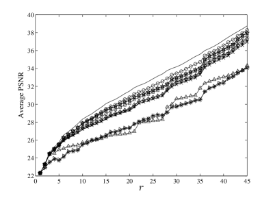
\psfrag{aaaa}{\scriptsize DCT}\psfrag{bbbb}{\scriptsize$\mathbf{T}_{0}$}\psfrag{cccc}{\scriptsize$\mathbf{T}_{1}$}\psfrag{dddd}{\scriptsize$\mathbf{T}_{2}$}\psfrag{eeee}{\scriptsize$\mathbf{T}_{3}$}\psfrag{ffff}{\scriptsize$\mathbf{T}_{4}$~{}\cite[cite]{[\@@bibref{}{cb2011}{}{}]}}\psfrag{gggg}{\scriptsize$\mathbf{T}_{5}$}\psfrag{hhhh}{\scriptsize$\mathbf{T}_{6}$~{}\cite[cite]{[\@@bibref{}{multibeam2012}{}{}]}}\psfrag{iiii}{\scriptsize$\mathbf{T}_{7}$}\psfrag{jjjj}{\scriptsize$\tilde{\mathbf{T}}_{1}$}\psfrag{kkkk}{\scriptsize$\tilde{\mathbf{T}}_{2}$~{}\cite[cite]{[\@@bibref{}{haweel2001new}{}{}]}}\psfrag{llll}{\scriptsize$\tilde{\mathbf{T}}_{3}$}\includegraphics[width=208.13574pt]{ssim}

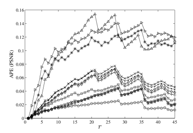
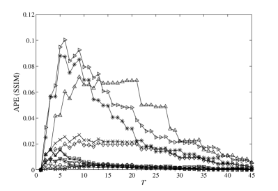
Figure 2: Quality measures of the considered approximations for several values of $r$ according to the following figures of merit: 2 Average PSNR, 2 Average SSIM, 2 Average PSNR absolute percentage error relative to the DCT, and 2 Average SSIM absolute percentage error relative to the DCT.

Approximation $\mathbf{T}_{7}$ outperformed all other approximations. This is partially expected because, by using all possible elements in $\mathcal{C}$, it may potentially better approximate the actual DCT vector basis. Nevertheless, it should be noticed that $\mathbf{T}_{7}$ also possesses the highest computational cost among the examined transformations. On the other hand, approximation $\tilde{\mathbf{T}}_{1}$ has the lowest computational complexity, requiring only 18 additions. The orthogonal approximation $\mathbf{T}_{3}$ showed comparable performance to the non-orthogonal approximation $\tilde{\mathbf{T}}_{3}$. However, the non-orthogonal approximation is less computationally expensive requiring 28 additions and 10 bit-shifts; whereas $\mathbf{T}_{3}$ requires 30 additions and 16 bit-shifting operations. Comparing the approximations with 22 additions, we have that $\mathbf{T}_{0}$ could outperform approximations $\mathbf{T}_{1}$ and $\mathbf{T}_{2}$ in terms of PSNR and SSIM measures for all considered values of $r$. In terms of the approximations with 24 additions, we have that $\mathbf{T}_{4}$ showed better behavior than approximations $\mathbf{T}_{5}$ and $\mathbf{T}_{6}$ according to both measures. Moreover, $\mathbf{T}_{4}$ requires no bit-shifting operations. Focusing on the non-orthogonal transforms, $\tilde{\mathbf{T}}_{3}$ presented the best performance in terms of PSNR and SSIM measures. However, $\tilde{\mathbf{T}}_{1}$ and SDCT showed lower computational complexity.

The preceding discussion permit us to identify the approximations with better performance and complexity trade-off. Thus, we separate the following approximations: $\tilde{\mathbf{T}}_{1}$, $\tilde{\mathbf{T}}_{3}$, $\mathbf{T}_{0}$, and $\mathbf{T}_{4}$. Considering this restricted set of transformations, we processed two particular images for qualitative analysis. The SDCT and DCT were also considered for comparison purposes. Fig. 6.2 and 6.2 shows ‘boat’ and ‘Lena’ images after being submitted to the JPEG-like compression experiment for $r=10$ and $r=25$, respectively. PSNR and SSIM measurements are also included.

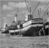
(a) $\mathbf{T}_{0}$ (PSNR=27.862, SSIM=0.955)

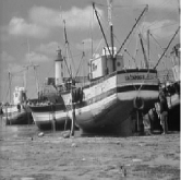
(b) $\mathbf{T}_{4}$ [17] (PSNR=27.870, SSIM=0.968)

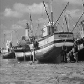
(d) $\tilde{\mathbf{T}}_{2}$ [23] (PSNR=25.760, SSIM=0.915)

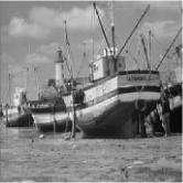
(e) $\tilde{\mathbf{T}}_{3}$ (PSNR=28.416, SSIM=0.967)

(f) DCT (PSNR=28.972, SSIM=0.970)

Figure 3: Compressed ‘boat’ image using 3(a) $\mathbf{T}_{0}$, 3(b) $\mathbf{T}_{4}$ [17], LABEL:boat_t0_til $\tilde{\mathbf{T}}_{1}$, 3(d) $\tilde{\mathbf{T}}_{2}$ [23], 3(e) $\tilde{\mathbf{T}}_{3}$, and 3(f) DCT, for $r=10$.

(a) $\mathbf{T}_{0}$ (PSNR=34.138, SSIM=0.989)

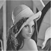
(b) $\mathbf{T}_{4}$ [17] (PSNR=34.159, SSIM=0.996)

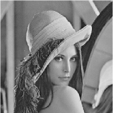
(d) $\tilde{\mathbf{T}}_{2}$ [23] (PSNR=31.852, SSIM=0.989)

(e) $\tilde{\mathbf{T}}_{3}$ (PSNR=35.157, SSIM=0.996)

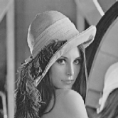
(f) DCT (PSNR=37.886, SSIM=0.997)

Figure 4: Compressed ‘Lena’ image using 4(a) $\mathbf{T}_{0}$, 4(b) $\mathbf{T}_{4}$ [17], LABEL:lena_t0_til $\tilde{\mathbf{T}}_{1}$, 4(d) $\tilde{\mathbf{T}}_{2}$ [23], 4(e) $\tilde{\mathbf{T}}_{3}$, and 4(f) DCT, for $r=25$.

7 Conclusion

This paper introduces a collection of DCT approximations derived from the application of common integer functions to the exact DCT. The proposed mathematical formalism could encompass—as particular cases—several transforms already archived in literature. In particular, the well-known SDCT was derived in a systematic way. All proposed transforms were given fast algorithms, which have the same structure. This suggest a common mathematical structure among all discussed approximations. Only additions and simple bit-shifting operations were necessary for their evaluation. Such low-complexity character of the obtained approximations makes them suitable for hardware implementation in dedicated architecture employing fixed-point arithmetic. The proposed approximations were assessed in terms of computational complexity and performance in JPEG-like compression; exhibiting a good balance between cost and performance.

References

- [1] N. Ahmed, T. Natarajan, and K. R. Rao, Discrete cosine transform, IEEE Transactions on Computers, C-23 (1974), pp. 90–93.
- [2] Y. Arai, T. Agui, and M. Nakajima, A fast DCT-SQ scheme for images, Transactions of the IEICE, E-71 (1988), pp. 1095–1097.
- [3] F. M. Bayer and R. J. Cintra, Image compression via a fast DCT approximation, IEEE Latin America Transactions, 8 (2010), pp. 708–713.
- [4] , DCT-like transform for image compression requires 14 additions only, Electronics Letters, 48 (2012), pp. 919–921.
- [5] F. M. Bayer, R. J. Cintra, A. Edirisuriya, and A. Madanayake, A digital hardware fast algorithm and FPGA-based prototype for a novel 16-point approximate DCT for image compression applications, Measurement Science and Technology, 23 (2012), p. 114010.
- [6] V. Bhaskaran and K. Konstantinides, Image and Video Compression Standards, Kluwer Academic Publishers, Boston, 1997.
- [7] R. E. Blahut, Fast Algorithms for Signal Processing, Cambridge University Press, 2010.
- [8] F. Bossen, B. Bross, K. Suhring, and D. Flynn, HEVC complexity and implementation analysis, IEEE Transactions on Circuits and Systems for Video Technology, 22 (2012), pp. 1685–1696.
- [9] S. Bouguezel, M. O. Ahmad, and M. N. S. Swamy, Low-complexity 88 transform for image compression, Electronics Letters, 44 (2008), pp. 1249–1250.
- [10] , A multiplication-free transform for image compression, in 2nd International Conference on Signals, Circuits and Systems, Nov. 2008, pp. 1–4.
- [11] , A fast 88 transform for image compression, in International Conference on Microelectronics (ICM), Dec. 2009, pp. 74–77.
- [12] , A novel transform for image compression, in 53rd IEEE International Midwest Symposium on Circuits and Systems (MWSCAS), Aug. 2010, pp. 509–512.
- [13] , A low-complexity parametric transform for image compression, in IEEE International Symposium on Circuits and Systems (ISCAS), 2011.
- [14] , Binary discrete cosine and Hartley transforms, IEEE Transactions on Circuits and Systems I: Regular Papers, 60 (2013), pp. 989–1002.
- [15] V. Britanak, P. Yip, and K. R. Rao, Discrete Cosine and Sine Transforms, Academic Press, 2007.
- [16] R. J. Cintra, An integer approximation method for discrete sinusoidal transforms, Journal of Circuits, Systems, and Signal Processing, 30 (2011), pp. 1481–1501.
- [17] R. J. Cintra and F. M. Bayer, A DCT approximation for image compression, IEEE Signal Processing Letters, 18 (2011), pp. 579–582.
- [18] R. J. Clarke, Relation between the Karhunen-Loève and cosine transforms, IEEE Proceedings F Communications, Radar and Signal Processing, 128 (1981), pp. 359–360.
- [19] A. Edirisuriya, A. Madanayake, V. Dimitrov, R. J. Cintra, and J. Adikari, VLSI architecture for 8-point AI-based Arai DCT having low area-time complexity and power at improved accuracy, Journal of Low Power Electronics and Applications, 2 (2012), pp. 127–142.
- [20] E. Feig and S. Winograd, Fast algorithms for the discrete cosine transform, IEEE Transactions on Signal Processing, 40 (1992), pp. 2174–2193.
- [21] B. N. Flury and W. Gautschi, An algorithm for simultaneous orthogonal transformation of several positive definite symmetric matrices to nearly diagonal form, SIAM Journal on Scientific and Statistical Computing, 7 (1986), pp. 169–184.
- [22] R. L. Graham, D. E. Knuth, and O. Patashnik, Concrete Mathematics, Addison-Wesley, Upper Saddle River, NJ, 2nd ed., 2008.
- [23] T. I. Haweel, A new square wave transform based on the DCT, Signal Processing, 82 (2001), pp. 2309–2319.
- [24] M. T. Heideman and C. S. Burrus, Multiplicative complexity, convolution, and the DFT, Signal Processing and Digital Filtering, Springer-Verlag, 1988.
- [25] N. J. Higham, Computing real square roots of a real matrix, Linear Algebra and its Applications, 88/89 (1987), pp. 405–430.
- [26] H. S. Hou, A fast recursive algorithm for computing the discrete cosine transform, IEEE Transactions on Acoustic, Signal, and Speech Processing, 6 (1987), pp. 1455–1461.
- [27] Q. Huynh-Thu and M. Ghanbari, Scope of validity of PSNR in image/video quality assessment, Electronics Letters, 44 (2008), pp. 800–801.
- [28] International Organisation for Standardisation, Generic coding of moving pictures and associated audio information – Part 2: Video, ISO/IEC JTC1/SC29/WG11 - coding of moving pictures and audio, ISO, 1994.
- [29] International Organization for Standardization, ISO/IEC/IEEE 60559:2011, 2011.
- [30] International Telecommunication Union, ITU-T recommendation H.261 version 1: Video codec for audiovisual services at kbits, tech. rep., ITU-T, 1990.
- [31] , ITU-T recommendation H.263 version 1: Video coding for low bit rate communication, tech. rep., ITU-T, 1995.
- [32] S. Ishwar, P. K. Meher, and M. N. S. Swamy, Discrete Tchebichef transform - A fast algorithm and its application in image/video compression, in IEEE International Symposium on Circuits and Systems (ISCAS), 2008, pp. 260–263.
- [33] Joint Video Team, Recommendation H.264 and ISO/IEC 14 496–10 AVC: Draft ITU-T recommendation and final draft international standard of joint video specification, tech. rep., ITU-T, 2003.
- [34] S. M. Kay, Fundamentals of Statistical Signal Processing, Volume I: Estimation Theory, vol. 1 of Prentice Hall Signal Processing Series, Prentice Hall, Upper Saddle River, NJ, 1993.
- [35] B. G. Lee, A new algorithm for computing the discrete cosine transform, IEEE Transactions on Acoustics, Speech and Signal Processing, ASSP-32 (1984), pp. 1243–1245.
- [36] K. Lengwehasatit and A. Ortega, Scalable variable complexity approximate forward DCT, IEEE Transactions on Circuits and Systems for Video Technology, 14 (2004), pp. 1236–1248.
- [37] J. Liang and T. D. Tran, Fast multiplierless approximation of the DCT with the lifting scheme, IEEE Transactions on Signal Processing, 49 (2001), pp. 3032–3044.
- [38] M. C. Lin, L. R. Dung, and P. K. Weng, An ultra-low-power image compressor for capsule endoscope, BioMedical Engineering OnLine, 5 (2006), pp. 1–8.
- [39] C. Loeffler, A. Ligtenberg, and G. Moschytz, Practical fast 1D DCT algorithms with 11 multiplications, in Proceedings of the International Conference on Acoustics, Speech, and Signal Processing, 1989, pp. 988–991.
- [40] A. Luthra, G. J. Sullivan, and T. Wiegand, Introduction to the special issue on the H.264/AVC video coding standard, IEEE Transactions on Circuits and Systems for Video Technology, 13 (2003), pp. 557–559.
- [41] A. Madanayake, A. Edirisuriya, R. J. Cintra, V. S. Dimitrov, and N. T. Rajapaksha, A single-channel architecture for algebraic integer based 2-D DCT computation, IEEE Transactions on Circuits and Systems for Video Technology, PP (2013), pp. 1–1.
- [42] H. L. P. A. Madanayake, R. J. Cintra, D. Onen, V. S. Dimitrov, and L. T. Bruton, Algebraic integer based 2-D DCT architecture for digital video processing, in IEEE International Symposium on Circuits and Systems (ISCAS), 2011, pp. 1247–1250.
- [43] MATLAB, version 8.1 (R2013a) Documentation, The MathWorks Inc., Natick, Massachusetts, 2013.
- [44] K. Nakagaki and R. Mukundan, A fast 44 forward discrete Tchebichef transform algorithm, IEEE Signal Processing Letters, 14 (2007), pp. 684–687.
- [45] K. Oldham, J. Myland, and J. Spanier, An Atlas of Functions, Springer, 2 ed., 2008.
- [46] W. B. Pennebaker and J. L. Mitchell, JPEG Still Image Data Compression Standard, Van Nostrand Reinhold, New York, NY, 1992.
- [47] G. Plonka, A global method for invertible integer DCT and integer wavelet algorithms, Applied and Computational Harmonic Analysis, 16 (2004), pp. 90–110.
- [48] U. S. Potluri, A. Madanayake, R. J. Cintra, F. M. Bayer, and N. Rajapaksha, Multiplier-free DCT approximations for RF multi-beam digital aperture-array space imaging and directional sensing, Measurement Science and Technology, 23 (2012), p. 114003.
- [49] M. T. Pourazad, C. Doutre, M. Azimi, and P. Nasiopoulos, HEVC: The new gold standard for video compression: How does HEVC compare with H.264/AVC?, IEEE Consumer Electronics Magazine, 1 (2012), pp. 36–46.
- [50] N. Rajapaksha, A. Edirisuriya, A. Madanayake, R. J. Cintra, D. Onen, I. Amer, and V. S. Dimitrov, Asynchronous realization of algebraic integer-based 2D DCT using Achronix Speedster SPD60 FPGA, Journal of Electrical and Computer Engineering, 2013 (2013), pp. 1–9.
- [51] K. R. Rao and P. Yip, Discrete Cosine Transform: Algorithms, Advantages, Applications, Academic Press, San Diego, CA, 1990.
- [52] N. Roma and L. Sousa, Efficient hybrid DCT-domain algorithm for video spatial downscaling, EURASIP Journal on Advances in Signal Processing, 2007 (2007), pp. 30–30.
- [53] G. A. F. Seber, A Matrix Handbook for Statisticians, John Wiley & Sons, Inc, 2008.
- [54] G. J. Sullivan, J. Ohm, W.-J. Han, and T. Wiegand, Overview of the high efficiency video coding (HEVC) standard, IEEE Transactions on Circuits and Systems for Video Technology, 22 (2012), pp. 1649–1668.
- [55] The USC-SIPI image database. http://sipi.usc.edu/database/, 2011. University of Southern California, Signal and Image Processing Institute.
- [56] B. Vasudev and N. Merhav, DCT mode conversions for field/frame coded MPEG video, in IEEE Second Workshop on Multimedia Signal Processing, Dec. 1998, pp. 605–610.
- [57] M. Vetterli and H. Nussbaumer, Simple FFT and DCT algorithms with reduced number of operations, Signal Processing, 6 (1984), pp. 267–278.
- [58] G. K. Wallace, The JPEG still picture compression standard, IEEE Transactions on Consumer Electronics, 38 (1992), pp. xviii–xxxiv.
- [59] Z. Wang, Fast algorithms for the discrete W transform and for the discrete Fourier transform, IEEE Transactions on Acoustics, Speech and Signal Processing, ASSP-32 (1984), pp. 803–816.
- [60] Z. Wang, A. C. Bovik, H. R. Sheikh, and E. P. Simoncelli, Image quality assessment: from error visibility to structural similarity, IEEE Transactions on Image Processing, 13 (2004), pp. 600–612.
- [61] T. Wiegand, G. J. Sullivan, G. Bjontegaard, and A. Luthra, Overview of the H.264/AVC video coding standard, IEEE Transactions on Circuits and Systems for Video Technology, 13 (2003), pp. 560–576.
- [62] Wolfram Research, Round – nearest integer function. http://functions.wolfram.com/IntegerFunctions/Round/27/01/01/01/, Sept. 2013.