The VLT-FLAMES Tarantula Survey

Abstract

Context. The 30 Doradus (30 Dor) region of the Large Magellanic Cloud is the nearest starburst region. It contains the richest population of massive stars in the Local Group and it is thus the best possible laboratory to investigate open questions in the formation and evolution of massive stars.

Aims. Using ground based multi-object optical spectroscopy obtained in the framework of the VLT-FLAMES Tarantula Survey (VFTS), we aim to establish the (projected) rotational velocity distribution for a sample of 216 presumably single O-type stars in 30 Dor. The size of the sample is large enough to obtain statistically significant information and to search for variations among sub-populations – in terms of spectral type, luminosity class, and spatial location – in the field of view.

Methods. We measured projected rotational velocities, $\varv_{\rm e}\sin i$, by means of a Fourier transform method and a profile fitting method applied on a set of isolated spectral lines. We also used an iterative deconvolution procedure to infer the probability density, $\rm{P(\varv_{\rm e})}$, of the equatorial rotational velocity, $\varv_{\rm e}$.

Results. The distribution of $\varv_{\rm e}\sin i$  shows a two-component structure: a peak around 80 ${\rm km}\>{\rm s}^{-1}$ and a high-velocity tail extending up to $\sim$600 ${\rm km}\>{\rm s}^{-1}$. This structure is also present in the inferred distribution $\rm{P(\varv_{\rm e})}$ with around 80% of the sample having 0 $<$ $\varv_{\rm e}$  $\leq\,300$ ${\rm km}\>{\rm s}^{-1}$ and the other 20% distributed in the high-velocity region. The presence of the low-velocity peak is consistent with that found in other studies for late O- and early B-type stars.

Conclusions. Most of the stars in our sample rotate with a rate less than 20% of their break-up velocity. For the bulk of the sample, mass-loss in a stellar wind and/or envelope expansion is not efficient enough to significantly spin down these stars within the first few Myr of evolution. If massive-star formation results in stars rotating at birth with a large fraction of their break-up velocities, an alternative braking mechanism, possibly magnetic fields, is thus required to explain the present day rotational properties of the O-type stars in 30 Dor. The presence of a sizeable population of fast rotators is compatible with recent population synthesis computations that investigate the influence of binary evolution on the rotation rate of massive stars. Despite the fact that we have excluded stars that show significant radial velocity variations, our sample may have remained contaminated by post-interaction binary products. The fact that the high-velocity tail may be preferentially (and perhaps even exclusively), populated by post-binary interaction products, has important implications for the evolutionary origin of systems that produce gamma-ray bursts.

1 Introduction

The distribution of stellar rotation rates at birth is a ‘fingerprint’ of the formation process of a population of stars. For massive stars the rotational distribution is especially interesting because so little is known about how these stars form (e.g. Zinnecker & Yorke, 2007). Considerations of angular momentum conservation during the gravitational collapse of a molecular cloud suggest an ‘angular momentum problem’, i.e. it appears difficult for the forming stars – whether they be of low- or high-mass – not to rotate near critical velocities. However, very few massive O-type stars are known to be extreme rotators.

If massive stars form through disk accretion, in a similar way to low mass stars, their initial spin rates are likely controlled by gravitational torques (Lin et al., 2011). Only massive stars that have low accretion rates, long disk lifetimes, weak magnetic coupling with the disk, and/or surface magnetic fields that are significantly stronger than what current observational estimates suggest, may have their initial spin regulated by magnetic torques (Rosen et al., 2012). Perhaps in these cases, intrinsic slow rotators can be formed.

The initial rotation rate is also one of the main properties affecting the evolution of a massive star. For instance, rotation induces internal mixing and prolongs the main-sequence life time (see Maeder & Meynet, 2000; Brott et al., 2011a; Ekström et al., 2012). A very high initial rotation rate may cause rotational distortion and gravity darkening (Collins, 1963; Collins & Harrington, 1966) and may even lead to homogeneous evolution (Maeder, 1980; Brott et al., 2011a, b). In low-metallicity environments this type of evolution has been suggested to lead to gamma-ray-bursts (Yoon & Langer, 2005; Woosley & Heger, 2006).

With the above science topics in mind, considerable effort has been invested in establishing the full distribution of equatorial rotational velocities ($\varv_{\rm e}$) of massive stars. Spectroscopic studies provide projected rotational velocities ($\varv_{\rm e}\sin i$, where $i$ is the inclination angle of the stellar rotation axis with respect to the line-of-sight). Large populations are thus preferred in order to confidently deconvolve the observed distribution and obtain a true $\varv_{\rm e}$ distribution (Penny, 1996; Huang & Gies, 2006; Hunter et al., 2008; Penny & Gies, 2009; Huang et al., 2010; Dufton et al., 2013). Obviously, the current values of spin rates do not necessarily reflect initial values. Stellar expansion and/or angular momentum loss via stellar winds are proposed mechanisms that spin down stars as time passes. Both these mechanisms, however, seem rather ineffective for the bulk of the massive stars. Internal redistribution of angular momentum effectively prevents the spin down of the surface layers as the star evolves to larger main-sequence radii and mass loss seems only effective for stars more massive than 40 $\mathit{M}_{\odot}$ at birth (Brott et al., 2011a, b; Vink et al., 2010, 2011).

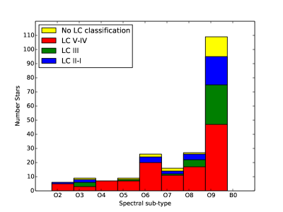
Figure 1: Spatial distribution (SpT) distribution of the O-type stars in our sample, binned per spectral sub-type. Different colors indicate different Luminosity Class (LC) (see legend).

As the intrinsic multiplicity fraction of massive stars at birth seems very high (Sana et al., 2012), it is also important to consider the effects of binary evolution on the rotational properties. Interestingly enough, binary interaction quite often occurs early on in the evolution of these systems, with up to 40% of all stars born as O-type stars being affected before leaving the main sequence (Sana et al., 2012). Using the intrinsic binary properties of Galactic O-type stars (Sana et al., 2012), de Mink et al. (2013) show that binary interaction strongly impacts spin rates, producing a ‘high-velocity tail’ in the $\varv_{\rm e}\sin i$ distribution through angular momentum transfer processes. Though studies of O-type star populations often try to select samples from which the known binaries have been removed, de Mink et al. (in prep.) show that such samples likely remain strongly contaminated by (unidentified) binary interaction products. Whether the results of de Mink et al. are consistent with all rapidly ($\varv_{\rm e}\,>200-300$ ${\rm km}\>{\rm s}^{-1}$) spinning O-type stars being spun-up binary products is an intriguing question. A positive answer may imply that the proposed homogeneous single-star channel to gamma-ray-bursts mentioned above does not occur in nature.

The VLT-FLAMES Tarantula Survey (VFTS) is a multi-epoch spectroscopic campaign targeting over 800 massive O and and early-B stars across the 30 Doradus (30 Dor) region in the Large Magellanic Cloud (LMC), including targets in the OB clusters NGC 2070 and NGC 2060. The distance to 30 Dor is well constrained (Gibson, 2000) and its foreground extinction is relatively low (see Evans et al., 2011, hereafter Paper I). The large massive-star population is ideal for studying the rotational velocity distribution. The low metal content of the LMC is in this sense even beneficial, as for such an environment the tail of the $\varv_{\rm e}\sin i$ distribution produced by binary effects is expected to be more extended and pronounced (de Mink et al., 2013).

The dense core cluster of the Tarantula Nebula, Radcliffe 136 (R136), has a likely age of 1-2 Myr (de Koter et al., 1998; Massey & Hunter, 1998), but may actually be a composite of two sub-clusters (Sabbi et al., 2012), with a third population that is a few million years older nearby (Selman et al., 1999). The very central regions were excluded from the VFTS because of crowding issues. A series of distinct populations, with varying ages reaching up to $\sim$25 Myr, can be distinguished in the Tarantula field (Walborn & Blades, 1997), suggesting that 30 Dor has been continuously forming massive stars over the last 25 Myr, although probably with a variable formation rate.

The key questions we want to address in this study are: how are the rotational velocities of O-type stars in 30 Dor distributed? Which fraction of the stars are slow rotators? Does the distribution have a high-velocity tail? If present, is the distribution of rapid rotators suggestive of a contribution of unidentified binaries? The layout of the paper is as follows. Section 2 describes the selection of our sample. The methodology and the results from different diagnostic lines are described in Section 3. Section 4 presents the $\varv_{\rm e}\sin i$ and $\varv_{\rm e}$ distributions. The results are discussed in Section 5 and our conclusions are summarized (Section 6).

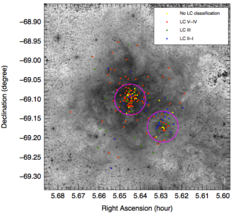
Figure 2: SpT of the presumably single O-type stars as a function of the LC. The circles define regions within 2.4’ of NGC 2070 (central circle) and NGC 2060 (SW circle). Colors have the same meaning as in Fig. 1 (only available in the online version).

Figure 3: SpT of our sample in the 30 Dor field of view. Different colors identify the different groups listed in Table 1 and are identified in the legend.

2 Sample

The VFTS project and the data have been described in Paper I. Here, we focus on the presumably single O-type stars that have been observed using the Medusa fibers. The total Medusa sample contains 332 O-type objects. Sana et al. (2013, hereafter Paper VIII) have identified spectroscopic binaries from multi-epoch radial velocity (RV) measurements: 172 O-type stars show no significant RV variations and are presumably single; 116 objects show significant RV variations with a peak-to-peak amplitude ($\rm{\Delta RV}$) larger than 20 ${\rm km}\>{\rm s}^{-1}$ and are considered binaries. The remaining 44 objects show low-amplitude significant RV variations ($\rm{\Delta RV}\,\leq$ 20 ${\rm km}\>{\rm s}^{-1}$ ). The latter variations may be the result of photospheric activity (pulsations and/or wind variability) or indicate a spectroscopic binary system. In Paper VIII, we estimated that photospheric variations and genuine binaries contribute to the low-amplitude RV variation sample in roughly equal portions. To avoid biasing our analysis against supergiants, which are expected to show spectroscopic variability (see e.g. Simón-Díaz et al., 2010), we include these 44 low-amplitude RV variable objects in our sample, reaching thus a total sample size of 216 O-type stars.

Because of the limited number of observing epochs, a subset of stars in our RV-constant sample are expected to be undetected binaries. Given the VFTS binary detection probability among O-type stars (of $\approx$ 0.7, Paper VIII, ), one estimates that this may be the case for up to about 25% of our single-star sample. Undetected binaries are preferentially wide and/or low-mass ratio systems (see sect. 3 in Paper VIII). Tidal interactions are thus expected to be negligible for these systems so that the measurement of the rotational velocity of the main component should be mostly unaffected by the binary status.

The spectral classifications of the O-type stars in the VFTS will be presented in Walborn et al. (in prep.). Fig. 1 shows the spectral type (SpT) and luminosity class (LC) distribution for our sample, which is dominated by O9-O9.7 stars (52% of the sample size) and by dwarfs and sub-giants (LC V-IV). As indicated in Fig. 1, a luminosity classification is missing for 22 stars, i.e. about 10 % of our sample. For seven stars the precise spectral type has not been established either due to the poor signal to noise ratio ($\rm{S/N}$) and/or heavy nebular contamination. These seven stars have been excluded from Fig. 1 but are still incorporated in our analysis.

The spatial distribution of our sample is shown in Fig. 2. The field of view is dominated by the central cluster NGC 2070. A circle of radius 2.4’ (or 37 pc) around the cluster center contains 105 stars from our sample: 62 are of LC V-IV, 15 are LC III and 28 are LC II-I. A second concentration of 45 O-type stars is found in a similar sized region around the NGC 2060 cluster, located about 6’ to the south-west of NGC 2070. NGC 2060 is somewhat older than NGC 2070 (Walborn & Blades, 1997). Accordingly, it contains a larger fraction of LC II-I stars (23 %) than NGC 2070 (9 %). The remaining stars, throughout the paper referred to as the stars outside clusters, are spread throughout the field of view. These may originate from either NGC 2070 or 2060, but may also have formed in other star-forming events in the 30 Doradus region at large.

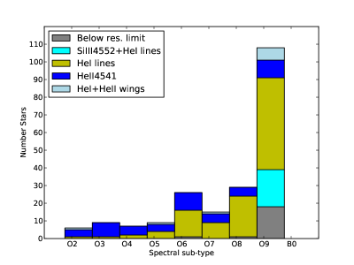
Figure 4: Diagnostic lines used as a function of the SpT of the stars in our sample.

3 Measuring the projected rotational velocity

3.1 Methodology

The projected rotational velocity ($\varv_{\rm e}\sin i$) of stars can be measured directly from the broadening of their spectral lines (Carroll, 1933; Gray, 1976). Commonly used methods for OB-type stars include direct measurement of the full width at half maximum (FWHM; Slettebak et al., 1975; Herrero et al., 1992; Abt et al., 2002, e.g.), cross-correlation of the observed spectrum against a template spectrum (e.g. Penny, 1996; Howarth et al., 1997), and comparison with synthetic lines calculated from model atmospheres (e.g. Mokiem et al., 2006). In this study we use a Fourier Transform (FT) method and a line profile fitting method which we refer to as the Goodness of Fit (GOF) method. Both methods are applied to a set of suitable spectral lines present in the VFTS Medusa LR02 and LR03 spectra (see Section 3.2). A comparison of the measurements obtained from both methods allows us to verify the internal consistency of the derived values.

The FT method is explained in Gray (1976). It has been systematically applied to OB-type stars by Ebbets (1979) and Simón-Díaz & Herrero (2007). In summary, the first minimum of the Fourier spectrum uniquely identifies the value of $\varv_{\rm e}\sin i$. One advantage of the FT method is that the derived $\varv_{\rm e}\sin i$  value is in principle not strongly affected by the presence of photospheric velocity fields, such as macro-turbulent motions. However, the method encounters difficulties in case of strong nebular contamination, poor $\rm{S/N}$, weak lines, and/or when the rotational broadening contribution is of the order of the intrinsic broadening of the line.

The GOF method (e.g. Ryans et al., 2002; Simón-Díaz et al., 2010) adjusts a synthetic line profile to the observed profile using a least-square fit, taking into account the intrinsic, instrumental, rotational, and macro-turbulent broadening contributions through successive convolutions. In this study we neglect the intrinsic width of the spectral lines, effectively adopting a delta function for the intrinsic profile. The latter is then convolved with an instrumental (Gaussian) function that preserves the equivalent width (EW). For the rotational and macro-turbulent profiles, we follow the description given by Gray (1976). The rotational profile assumes a linear limb darkening law. We finally use a radial-tangential (RT) model parametrized with the quantity $\Theta_{\mathrm{RT}}$ as an appropriate representation of the macro-turbulent profile.

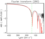
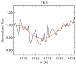
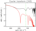
Figure 5: Example of the GOF and FT measurement methods applied to the He i $\rm{\lambda}$4713 line of VFTS 280 (top row, high $\rm{S/N}$) and VFTS 163 (bottom row, poor $\rm{S/N}$), to illustrate two different data qualities. Left-hand column: line profile (black) and its GOF solution (red). Right-hand column: Fourier transform of the observed spectrum (black) and of the best fit GOF profile (red). The dashed lines indicate the position of the FT first minimum.

3.2 Diagnostic lines

In general, different diagnostic lines do not provide the same accuracy in the $\varv_{\rm e}\sin i$ measurements. Metallic lines do not suffer from strong Stark broadening nor from nebular contamination and hence are best for obtaining $\varv_{\rm e}\sin i$ estimates. Si iii $\lambda$4552 is the only suitable metal line in our data set for these purposes. Unfortunately, it is only present in 6% of the sample and restricted to late spectral sub-types. Next in line in terms of reliability are nebular free or weakly contaminated He i lines, notably He i $\rm{\lambda}$4713, 4922, 4387, and 4471. By using the neutral helium lines we can study an additional 54% of the sample (see Table 1).

The remaining sample of stars (31%) suffers from strong nebular contamination, features only weak He i lines or – for the earliest spectral sub-types – does not show these lines at all. In those cases, amounting to 26% of our sample, we relied on He ii $\rm{\lambda}$4541. Finally, 14 stars present strong nebular contamination in He i, weak He ii lines and no Si iii line. We have estimated $\varv_{\rm e}\sin i$  for these sources by comparing rotationally broadened synthetic line profiles calculated using FASTWIND (Puls et al., 2005) to the wings of He i and He ii lines. Though FASTWIND does not take into account macro-turbulent broadening it, at least, allows us to derive upper limits on $\varv_{\rm e}\sin i$ for this small subset of stars.

The assumption of a delta-function for the intrinsic profile ignores a possible contribution of Stark broadening (more relevant for He i and He ii lines). Being conscious of that, we scrutinize the reliability of these lines for $\varv_{\rm e}\sin i$ determinations in Sect. 3.4. For practical purposes we refer to the group of stars for which the Si iii $\lambda$4552 and/or nebular free He i lines can be used as Group A and the remaining sample as Group B. Group A is thus identifying the stars for which the highest quality diagnostic lines are available, while Group B has diagnostics of a lower quality.

The resolving power of the VFTS Medusa LR02 and LR03 is $\sim$  0.6 $\AA$ (Paper I), corresponding to 40 ${\rm km}\>{\rm s}^{-1}$. We have adopted this value as our resolution limit and hence, when a $\varv_{\rm e}\sin i$ measurement is below 40 ${\rm km}\>{\rm s}^{-1}$ the corresponding star is systematically assigned to the 0–40 ${\rm km}\>{\rm s}^{-1}$ bin (see Sect. 4) without further indication of the specific $\varv_{\rm e}\sin i$ value.

Fig. 3 shows the spatial distribution of stars below the resolution limit and of stars in Groups A and B. Group A stars are spread out within the two clusters and show a lower fraction in the field of view. Group B stars are mainly concentrated in NGC 2070. There are two reasons that can explain this difference. First, part of the NGC 2070 cluster lies behind a filament of nebular gas, therefore contamination is stronger. Second, NGC 2070 is younger and, pro rata, contains more hot early O-type stars that show neither Si iii nor He i lines in their spectra.

Fig. 4 shows the spectral lines used for $\varv_{\rm e}\sin i$  measurements as a function of SpT. For late SpT, measurements are mostly obtained from He i, while He ii $\rm{\lambda}$4541 is increasingly used for earlier SpT. Stars with $\varv_{\rm e}\sin i$  below the resolution limit and stars featuring the Si iii $\lambda$4552 line are almost exclusively late O-type stars. Additionally, all stars showing Si iii also display at least one suitable He i line. The accuracy of, and the systematics between, $\varv_{\rm e}\sin i$ measurements obtained from both methods and for the different lines are discussed in the next subsections.

Table 1: Overview of the diagnostic lines used to derive the projected rotational velocity. Group A diagnostics provide the most reliable measurements; those in Group B are of a lesser quality. The last column lists the fraction of our sample for which each diagnostic can be applied.

Group	line	Sample (%)
	Below the resolution limit	9%
A	Si iii $\lambda$4552+He i lines	6%
A	He i $\rm{\lambda}$4713	}43mm[$54\%$]
A	He i $\rm{\lambda}$4922
A	He i $\rm{\lambda}$4387
A	He i $\rm{\lambda}$4471
Total Group A		60%
B	He ii $\rm{\lambda}$4541	25%
B	He i+He ii wings	6%
Total Group B		31%

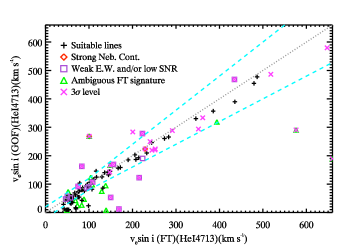
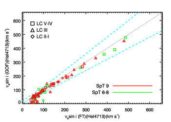
Figure 6: Comparison of $\varv_{\rm e}\sin i$ values obtained from the FT and GOF methods for He i $\rm{\lambda}$4713. Upper panel: Different symbols indicate different data quality, identified in the legend. Lower panel: Same as above after discarding the lower quality data. Information on the LC and SpT of the targets is provided by the symbol shapes and colors (see legend). In both panels, the dotted lines indicates the 1:1 relation. The dashed lines show the $\pm 20$ ${\rm km}\>{\rm s}^{-1}$ and/or $\pm\,20$%, whichever is the largest, around the 1:1 relation.

3.3 Comparison of results from FT and GOF methods

An example of FT and GOF $\varv_{\rm e}\sin i$ measurements for the He i $\rm{\lambda}$4713 line is presented in Fig. 5 for two different data qualities. In the upper panel the derived $\varv_{\rm e}\sin i$ from the FT and the GOF methods are in agreement. In the lower panel, the noise is affecting the FT, resulting in an erroneous $\varv_{\rm e}\sin i$ value while the correct $\varv_{\rm e}\sin i$ value is associated with the shallow FT minimum at $\sim$ 200 ${\rm km}\>{\rm s}^{-1}$. The combined investigation of results from FT and GOF methods hence helps to identify the more ambiguous cases which must be explored in more detail.

The upper panel in Fig. 6 compares $\varv_{\rm e}\sin i$ values obtained from applying the FT and GOF methods to the He i $\rm{\lambda}$4713 line. This plot includes all stars in our sample in which the He i $\rm{\lambda}$4713 line is detected and the $\varv_{\rm e}\sin i$ (FT) measurements are above the resolution limit (i.e. 116 stars). In addition to the full set of good quality measurements, different symbols are used to highlight various cases: (i) strong nebular contamination, (ii) low $\rm{S/N}$ ($<60$) and/or a comparatively weak diagnostic line (EW $\leq$ 50 m$\AA$), (iii) ambiguous first minimum in Fourier space (this is, for example, the case for VFTS163 in Fig. 5), and (iv) a central depth of the absorption-line profile that is smaller than three times the noise level. These explain all but 14 deviating points, which correspond to cases in which $\varv_{\rm e}\sin i$ (GOF) is below the resolution limit and $\varv_{\rm e}\sin i$ (FT) $>$ $\varv_{\rm e}\sin i$ (GOF). This behaviour is expected when the rotational broadening contribution to the line profile is similar to the intrinsic broadening and the $\rm{S/N}$ is not sufficiently high. In this situation the FT of the line may result in a spurious first zero, which is moved to higher values of $\varv_{\rm e}\sin i$ compared to the FT’s true first zero (see e.g. Simón-Díaz & Herrero, 2007). In these specific cases $\varv_{\rm e}\sin i$ (FT) measurements must be considered as upper limits for the actual projected rotational velocity. Save for one instance, these cases occur when $\varv_{\rm e}\sin i$  $\leq$ 80 ${\rm km}\>{\rm s}^{-1}$.

Once the poorer quality measurements resulting from cases (i) to (iv) are left aside, the $\varv_{\rm e}\sin i$ measurements for the 76 stars left in our comparison show a large degree of agreement between FT and GOF estimates over the full range of velocities, save for $\varv_{\rm e}\sin i$ measurements close to the spectral resolution limit (Fig. 6, bottom panel). Similar conclusions about the large degree of agreement between FT and GOF estimates can be drawn for the other He i lines and from Si iii $\lambda$4552. From now on the analysis will be presented excluding poor quality measurements.

The situation is, however, less clear for measurements based on He ii $\rm{\lambda}$4541 (Fig. 7, 101 stars). Above 150 ${\rm km}\>{\rm s}^{-1}$ the FT and GOF measurements agree to within 20%. A significant dispersion is, however, observed at lower velocities, with FT resulting in systematically higher $\varv_{\rm e}\sin i$ values than GOF. The origin of the observed systematics is discussed further in Section 3.4.2.

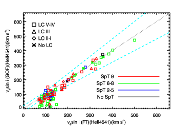
Figure 7: Comparison of the $\varv_{\rm e}\sin i$ measurements from the FT and GOF methods for He ii $\rm{\lambda}$4541. Information on the LC and SpT of the targets is provided by the symbol shapes and colors. Lines have the same meaning as in Fig. 6.

3.4 Comparison of results from the different diagnostic lines

In this section we compare the $\varv_{\rm e}\sin i$  measurements obtained from different diagnostic lines (Table 3). Figs. 8 to 10 show different cases of these comparisons and Table 2 summarizes the degree of agreement between the lines that have been investigated. Only $\varv_{\rm e}\sin i$  measurements that fulfill the quality criteria outlined in Sect. 3.3 are considered.

3.4.1 Si iii $\lambda$4552 and He i lines

Fig. 8 compares the $\varv_{\rm e}\sin i$ values obtained from Si iii $\lambda$4552 and He i $\rm{\lambda}$4713 for 12 stars. Measurements from both lines agree within $\pm$ 20 %  and/or $\pm$ 20 ${\rm km}\>{\rm s}^{-1}$, whichever is the largest, in over 90% of the cases. A similar degree of agreement is observed between FT measurements of He i $\rm{\lambda}$4713 and He i $\rm{\lambda}$4922 (Fig. 9) : 53 of the 58 stars displaying both lines again agree within $\pm$ 20% and/or $\pm$ 20 ${\rm km}\>{\rm s}^{-1}$, hence about 91% of the sample. We conclude that the comparison between $\varv_{\rm e}\sin i$ measurements obtained from Si iii and from different He i lines (Figs. 8, 9 and Table 2) reveals no systematic differences. This justifies the grouping of all the measurements from stars in Group A, irrespectively of the diagnostic line from which they have been obtained.

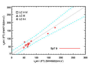
Figure 8: Comparison of $\varv_{\rm e}\sin i$ values from the FT method for He i $\rm{\lambda}$4713 and Si iii $\lambda$4552. Information on the LC and SpT of the targets is provided by the symbol shapes and colors. Lines have the same meaning as in Fig. 6.

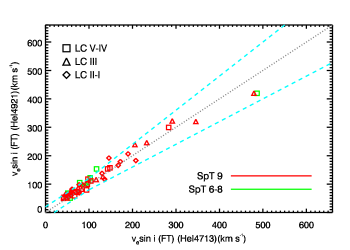
Figure 9: Comparison of $\varv_{\rm e}\sin i$ obtained from the FT method for He i $\rm{\lambda}$4922 and He i $\rm{\lambda}$4713. Information on the LC and SpT of the targets is provided by the symbol shapes and colors. Lines have the same meaning as in Fig. 6.

3.4.2 He ii $\rm{\lambda}$4541

As discussed in Sect. 3.3, the FT and GOF measurements obtained from the He ii $\rm{\lambda}$4541 line show a general agreement well within the 20% for $\varv_{\rm e}\sin i$  $\geq$ 150 ${\rm km}\>{\rm s}^{-1}$ (Fig. 7). However, the larger dispersion and systematics observed below 150 ${\rm km}\>{\rm s}^{-1}$ cast some doubts on the reliability of the He ii $\rm{\lambda}$4541 measurements for slow rotators. In this section we further explore this issue by comparing the He ii $\rm{\lambda}$4541 rotational velocities with those obtained from He i lines for those stars in Group A that display both He i and He ii lines. This comparison will allow us to decide which of our two methodologies provides the more reliable $\varv_{\rm e}\sin i$ information for Group B stars.

Fig. 10 (upper panel) compares $\varv_{\rm e}\sin i$  measured from He ii $\rm{\lambda}$4541 and from He i $\rm{\lambda}$4713 using the FT method. In the low-velocity domain ($\varv_{\rm e}\sin i\,<150$ ${\rm km}\>{\rm s}^{-1}$), FT values from He ii $\rm{\lambda}$4541 are systematically larger by about 30 ${\rm km}\>{\rm s}^{-1}$, on average, with a dispersion of about 23 ${\rm km}\>{\rm s}^{-1}$ compared to He i FT measurements. In this domain, the contribution of Stark broadening to the He ii $\rm{\lambda}$4541 line causes the power of the first lobe of the FT to diminish. As a consequence, the first zero is easily hidden within the white noise if the $\rm{S/N}$ is not high enough. The method then returns $\varv_{\rm e}\sin i$ values corresponding to the first FT zero that peaks out of the noise. This artificially moves the measurement to higher $\varv_{\rm e}\sin i$ values.

As illustrated in the lower panel of Fig. 10, the impact of the Stark broadening on our $\varv_{\rm e}\sin i$  measurements is partially mitigated by using the GOF rather than the FT method for He ii $\rm{\lambda}$4541. Although large deviations still occur in some cases, the average systematic difference in the measurements between He i and He ii drops off to 3 ${\rm km}\>{\rm s}^{-1}$, i.e. negligible in comparison with our expected accuracy. Using the GOF instead of the FT for He ii measurements thus allows to avoid a systematic bias in the measurements, leaving the derived $\varv_{\rm e}\sin i$ values only affected by random, though relatively large, uncertainties.

Table 2: Comparison between different diagnostic lines. Col. 1: figure index. Col. 2: total number of stars in the comparison. Cols. 3 and 4: diagnostic lines compared. Col. 5: number and fraction of stars in the comparison for which the measurements agree within 20% and/or 20 ${\rm km}\>{\rm s}^{-1}$, whichever is the largest. Measurements from the FT method are used, unless specified otherwise.

Fig.	Number	Diagnostic	Diagnostic	$\leq$ 20 ${\rm km}\>{\rm s}^{-1}$
	of stars	line 1	line 2	or $\leq$ 20 %
8	12	Si iii $\lambda$4552	He i $\rm{\lambda}$4713	11 (92%)
-	17	Si iii $\lambda$4552	He i $\rm{\lambda}$4387	14 (82%)
-	8	Si iii $\lambda$4552	He i $\rm{\lambda}$4471	7 (88%)
-	14	Si iii $\lambda$4552	He i $\rm{\lambda}$4922	13 (93%)
9	58	He i $\rm{\lambda}$4713	He i $\rm{\lambda}$4922	53 (91%)
-	66	He i $\rm{\lambda}$4387	He i $\rm{\lambda}$4713	57 (86%)
-	44	He i $\rm{\lambda}$4471	He i $\rm{\lambda}$4713	39 (86%)
-	52	He i $\rm{\lambda}$4387	He i $\rm{\lambda}$4471	43 (87%)
-	72	He i $\rm{\lambda}$4387	He i $\rm{\lambda}$4922	67 (93%)
-	46	He i $\rm{\lambda}$4387	He i $\rm{\lambda}$4471	41 (89%)
10 a)	31	He i $\rm{\lambda}$4713	He ii $\rm{\lambda}$4541	14 (45%)
-	40	He i $\rm{\lambda}$4387	He ii $\rm{\lambda}$4541	18 (45%)
-	31	He i $\rm{\lambda}$4471	He ii $\rm{\lambda}$4541	20 (65%)
-	31	He i $\rm{\lambda}$4471	He ii $\rm{\lambda}$4541	15 (48%)
10 b)	31	He i $\rm{\lambda}$4713	He ii $\rm{\lambda}$4541(GOF)	21 (68%)
-	40	He i $\rm{\lambda}$4387	He ii $\rm{\lambda}$4541(GOF)	21 (53%)
-	31	He i $\rm{\lambda}$4471	He ii $\rm{\lambda}$4541(GOF)	23 (74%)
-	31	He i $\rm{\lambda}$4471	He ii $\rm{\lambda}$4541(GOF)	23 (74%)

Table 3: Measured values of $\varv_{\rm e}\sin i$ (in ${\rm km}\>{\rm s}^{-1}$) for every star and diagnostic line. The ‘-’ sign indicates that the line has not been used. The full version of the table is available online.

VFTS	He i $\rm{\lambda}$4387	He i $\rm{\lambda}$4471	Si iii $\lambda$4552	He i $\rm{\lambda}$4713	He i $\rm{\lambda}$4922	He ii $\rm{\lambda}$4541
014	87	104	-	94	79	85
016	-	-	-	-	-	94
021	52	67	-	40	57	45
046	160	166	176	167	166	-
051	413	-	-	-	-	-
064	99	113	-	99	104	15
065	164	-	-	-	-	200
067	54	-	-	-	-	-
070	126	129	-	-	-	-
…	…	…	…	…	…	…

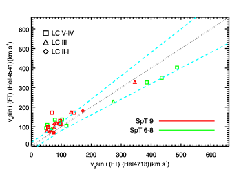
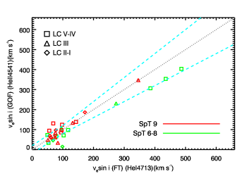
Figure 10: Comparison of $\varv_{\rm e}\sin i$ measurements from He i $\rm{\lambda}$4713 and He ii $\rm{\lambda}$4541. Upper panel: both diagnostic lines analysed using the FT method. Lower panel: He ii $\rm{\lambda}$4541 analyzed using the GOF and He i $\rm{\lambda}$4713 using the FT. Information on the LC and SpT of the targets is provided by the symbol shapes and colors. Lines have the same meaning as in Fig. 6.

In the high-velocity domain ($\varv_{\rm e}\sin i$  $>$ 250 ${\rm km}\>{\rm s}^{-1}$) a systematically lower $\varv_{\rm e}\sin i$ is obtained from He ii $\rm{\lambda}$4541 compared to He i $\rm{\lambda}$4713. The good agreement found between FT and GOF estimates for He ii $\rm{\lambda}$4541 in this $\varv_{\rm e}\sin i$ domain suggests that the difference is real and not related to a methodological bias. Fast rotation produces equatorial stretching of stars, which in turn induces a non-uniform surface gravity and temperature distribution (von Zeipel, 1924). In the particular case of fast rotating O-type stars, this means that the poles are hotter than the equator. As a consequence, photospheric regions closer to the pole (resp. equator) will contribute more to the formation of He ii (resp. He i) lines. Projected rotational velocities derived from He ii lines are thus expected to be lower than those from HeI lines, as observed in Fig. 10.

3.5 Measurement uncertainties

The methods that we have adopted to estimate $\varv_{\rm e}\sin i$ do unfortunately not provide measurement errors. We have estimated the typical accuracy of our measurements by examining the dispersions observed between measurements based on independent lines. We outline here the main conclusions. At low rotational velocities, absolute uncertainties provide a more sensible estimate of the true measurement error. At high rotational velocity, however, uncertainties are better expressed in relative terms.

For Group A stars, the root mean square (rms) dispersion between measurements from the different He i and Si iii lines amounts to about 10 ${\rm km}\>{\rm s}^{-1}$ for projected rotational velocities below 100 ${\rm km}\>{\rm s}^{-1}$ (see Figs. 8-9 and Table 2). It is of the order of 10% or better above 100 ${\rm km}\>{\rm s}^{-1}$. For Group B stars, the rms dispersion in the lower panel of the same figure indicates uncertainties not exceeding 30 ${\rm km}\>{\rm s}^{-1}$ below $\varv_{\rm e}\sin i=200$ ${\rm km}\>{\rm s}^{-1}$, and not exceeding 10% above 200 ${\rm km}\>{\rm s}^{-1}$ (see lower panel Fig. 10).

As pointed out in the previous section, our He ii measurements may underestimate the true rotational velocity of the stars for $\varv_{\rm e}\sin i$ $\geq$ 250  ${\rm km}\>{\rm s}^{-1}$. The five stars in Fig. 10 for which this is relevant indicate that the effect is probably of the order of 15–20%. Similarly, gravity darkening may cause our measurements to underestimate the true $\varv_{\rm e}\sin i$ at large rotational velocity (see also the discussion in Dufton et al., 2013, hereafter Paper X). Though both effects are not negligible, it will not affect our conclusion on the presence of a well-populated high-velocity tail in the rotational velocity distribution. Correcting these values would even strengthen that outcome.

As a last point, we note that most of the comparisons performed in this section concern mid- and late-O stars. The He i lines in early-O stars (O2-O5) are too weak to provide reliable $\varv_{\rm e}\sin i$ measurements, depriving us from an anchor point to test the quality of He ii-based $\varv_{\rm e}\sin i$ measurements. In Appendix A we compare $\varv_{\rm e}\sin i$ measurements obtained from He ii $\rm{\lambda}$4541 with those obtained from N v $\lambda$4604 for a small set of stars. We find that above 80 ${\rm km}\>{\rm s}^{-1}$, He ii and N v agree to within 10%. This adds confidence in the quality of $\varv_{\rm e}\sin i$ measurements for early-type Group B stars in that regime. The quality of the He ii-based $\varv_{\rm e}\sin i$ of early-O stars with $\varv_{\rm e}\sin i\mathrel{\hbox{\hbox to0.0pt{\hbox{\lower 4.0pt\hbox{$\sim$}}\hss}\hbox{$<$}}}80$ ${\rm km}\>{\rm s}^{-1}$ cannot be investigated further with the current data set and we thus adopt a formal uncertainty of 30 ${\rm km}\>{\rm s}^{-1}$ for these 15 stars.

3.6 Strategy for obtaining $\varv_{\rm e}\sin i$ estimates

Based on the analysis presented in Sect. 3.3 and 3.4 we have adopted the following strategy to obtain the final $\varv_{\rm e}\sin i$ measurements (see Table 4) for the full sample of 216 O-type stars:

• For those stars in Group A with FT measurements below 40 ${\rm km}\>{\rm s}^{-1}$, we adopt an upper limit of 40 ${\rm km}\>{\rm s}^{-1}$, and include them in the 0 – 40 bin of the $\varv_{\rm e}\sin i$ histograms (see Sect. 4).

• For those stars in Group A with FT measurements above 40 ${\rm km}\>{\rm s}^{-1}$, we compute a non-weighted average of the individual values obtained from the available He i and Si iii lines (see Table 3).

• For all stars in Group B where the He ii $\rm{\lambda}$4541 diagnostic line is available, we adopt the GOF measurement obtained from that line. If the obtained value is below 40 ${\rm km}\>{\rm s}^{-1}$, we consider the object below our resolution limit and assign it to the lowest velocity bin in our histograms.

• For the remaining 14 stars for which the above diagnostics can not be applied, we use the wings of the lines and compare them to synthetic spectra as described in Sect. 3.2.

While the GOF measurements of $\varv_{\rm e}\sin i$ based on He ii lines are good enough for the purposes of this study, individual values must be handled with care, as the measurements have a large dispersion. In particular, some of the Group B stars included in the first three bins of the $\varv_{\rm e}\sin i$ distributions presented in next sections may move between adjacent bins due to sizeable uncertainties. Because we verified earlier that there are no systematic effects, the larger uncertainties for some stars in Group B do not affect the overall distributions presented in this paper.

Table 4: Averaged $\varv_{\rm e}\sin i$  measurements and their 1$\sigma$ dispersion. The number of lines used and the category are also indicated. The full version of the table is available online.

VFTS	Group	$\varv_{\rm e}\sin i$  (${\rm km}\>{\rm s}^{-1}$)	$\sigma$ (${\rm km}\>{\rm s}^{-1}$)	# of lines
014	A	91	10	4
016	B	94	30	1
021	A	54	11	4
046	A	167	5	5
051	A	413	20	1
064	A	104	6	4
065	A	164	20	1
067	A	54	20	1
070	A	128	20	2
…	…	…	…	…

4 The $\varv_{\rm e}\sin i$ distribution

In this section, we construct and investigate the $\varv_{\rm e}\sin i$ distributions of the overall O-type star population within 30 Dor as well as within sub-populations of stars in our sample. We approximate the probability density function (pdf) using histograms with a bin size of 40 ${\rm km}\>{\rm s}^{-1}$. Such a bin size is consistent with our resolution limit (see Sect. 2) and is large enough to mitigate the effect of measurement uncertainties on the appearence of the histograms. Fig. 11 shows the overall $\varv_{\rm e}\sin i$ distribution. It is dominated by a clear peak at fairly low $\varv_{\rm e}\sin i$  and a well-populated high-velocity tail which extends continuously to 500 ${\rm km}\>{\rm s}^{-1}$. With a measured $\varv_{\rm e}\sin i$ of 609 and 610 ${\rm km}\>{\rm s}^{-1}$, VFTS 285 and VFTS 102 (Dufton et al., 2011), complete the projected rotational distributions at extreme rotation rates.

In the following sub-sections, we analyse the $\varv_{\rm e}\sin i$ distribution as a function of spatial location, LC and SpT. We use Kuiper tests (KP, Kuiper, 1960) to search for significant differences between the considered sub-populations. Results are reported in Table 5. Specifically, KP tests allow us to test the null hypothesis that two observed distributions are randomly drawn from the same parent population. Compared to the more widely used Kolmogorov-Smirnov test (KS, Kolmogorov, 1933), the KP test has the advantage to be similarly sensitivity to differences in the tails and around the median of the distributions while the KS test is known to be less sensitive if differences are located in the tails of the distribution. To support our discussion of the outcomes of the KP tests, we also show the cumulative distribution functions (cdf) because they provide a more direct view of the location of the differences between the distributions.

Figure 11: Histogram of the projected rotational velocities of our sample of 216 O-type stars in 30 Dor.

4.1 Spatial variations

Figure 12 shows the $\varv_{\rm e}\sin i$ distributions for stars in the NGC 2070 and NGC 2060 clusters and for stars outside these two clusters. Qualitatively all three distributions are similar with a peak in the low-velocity region and a high-velocity tail. The distributions for stars in the two clusters are statistically compatible. A KP test, however, indicates that the $\varv_{\rm e}\sin i$  distribution of stars outside the clusters shows differences with the NGC 2070 and NGC 2060 distributions, at the 9 and 3% significance level, respectively. For NGC 2070 the difference manifests itself in the high-velocity regime, the fraction of rapid rotators being larger outside of the clusters. For NGC 2060 both the low- and high-velocity region contribute to the significance of the differences detected by the KP test.

The difference in age between the two clusters, hence in the evolutionary stage of their O-type star population, does not seem to have strongly affected the $\varv_{\rm e}\sin i$ distribution of NGC 2060 compared to the younger NGC 2070. This suggests that standard evolutionary effects, such as spin down through wind mass-loss and/or envelope expansion are modest. The presence of a larger fraction of fast rotators outside clusters may, however, be linked to binary evolution if the field is relatively overpopulated with post-interaction objects. Binary interaction is indeed expected to produce rapidly rotating stars either through mass and angular momentum transfer to the secondary star during Roche lobe overflow or through the merging of the two components (de Mink et al., 2013). A relative overpopulation of the field can be obtained in two ways. Some of these binary products may have outlived their co-eval single star counterparts thanks to the rejuvenation effects resulting from the interaction process. Alternatively, post-interaction systems may have been ejected from their natal cluster when the primary experienced its supernova explosion. The correlation between rapid spin and large radial velocity of the field stars identified in the VFTS O-type star sample (Sana et al. in prep.) is an argument in favor of the latter scenario. This will be the topic of a separate investigation within the VFTS series of papers.

Qualitatively the origin of the lower number of slow rotators within NGC 2060 remains unclear. It may be related to the specific evolutionary stage of most of the stars in the clusters or reveal differences in the initial $\varv_{\rm e}\sin i$ distribution. The fact that dwarfs and sub-giants (LC V-IV) and bright giants and supergiants (LC II-I) have very similar distributions at low velocities (Fig. 13) tends to rule out differences in the evolutionary stage of the two clusters as a straightforward explanation.

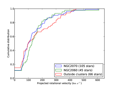
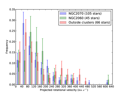
Figure 12: Cumulative (upper panel) and frequency (lower panel, with poisson error bars) distributions of the projected rotational velocities of the O-type stars for three spatially selected groups.

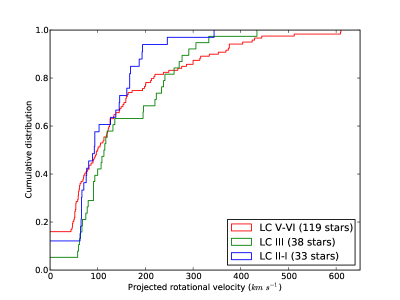
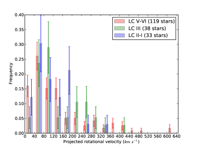
Figure 13: Cumulative (upper panel) and frequency (lower panel, with poisson error bars) distributions of the projected rotational velocities of the O-type stars for three different luminosity class categories.

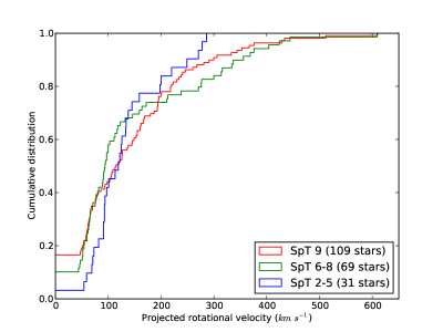
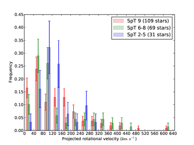
Figure 14: Cumulative (upper panel) and frequency (lower panel, with poisson error bars) distributions of the projected rotational velocities of the O-type stars for three different spectral type categories.

4.2 Luminosity Class

Figure 13 shows the $\varv_{\rm e}\sin i$ distributions for three luminosity groups: V-IV (119 stars), III (38 stars), and II-I (33 stars). There are 26 stars in our sample with no LC classification available and therefore we only used 190 stars. KP tests do not reveal statistically significant differences between the distributions of giants (LC III) and bright giants and supergiants (LC II-I). Both distributions are, however, statistically different from that of the dwarfs and sub-giants (LC V-IV), this latter group dominating the extreme of the high-velocity tail ($\varv_{\rm e}\sin i$ $\geq$ 450 ${\rm km}\>{\rm s}^{-1}$).

The difference in the high-velocity regime between the V-IV class and the other classes can be explained from evolutionary considerations. Following Weidner & Vink (2010) some 18% of our total sample presents masses above 40 $\mathit{M}_{\odot}$ (see Sect. 5.2). The bulk of our O-type star sample consists thus of main sequence stars initially less massive than about 40 $\mathit{M}_{\odot}$. For such stars the loss of angular momentum as a result of mass loss in a stellar wind is quite limited, therefore this is not expected to be an efficient mechanism for spin down (see Vink et al., 2010; Brott et al., 2011a). As the O-type stars evolve away from the zero-age main sequence their radii expand and one may naively expect to observe a spin down of the surface layers for more evolved stars. The spin down with increasing radius is however prevented by a simultaneous contraction of the stellar core and the efficient transport of angular momentum from the core to the envelope (Ekström et al., 2008; Brott et al., 2011a).

The critical rotation rate of a star, i.e. the maximum surface velocity above which the centrifugal force exceeds gravity, is, however, mostly defined by its size. Dwarfs are more compact than supergiants by about a factor two to three (Martins et al., 2005), which corresponds to break-up velocities a factor up to $\sqrt{3}$ larger. Break-up velocities for dwarfs and supergiants typical of our sample are around 700 and 400 ${\rm km}\>{\rm s}^{-1}$, respectively (de Mink et al., 2013). These estimates match well the maximum rotational velocities observed in Fig. 13. It also explains the absence of very rapid rotators among supergiants: such stars simply can not rotate faster than about 400 ${\rm km}\>{\rm s}^{-1}$.

The low-velocity region shows a lower frequency of giants compared to the other luminosity classes. Although the cause of this is unclear, possible explanations include different parent populations, different effects of the macroturbulent velocity field and/or low number statistics. Further investigations with higher-resolution data are needed to search for the origin of the observed paucity of giants with $\varv_{\rm e}\sin i$ $<$ 120 ${\rm km}\>{\rm s}^{-1}$.

Table 5: Kuiper tests (KP) statistics for different sets of the O-type stars (Cols. 1 and 2). The number of stars in every sub-sample are given in Cols. 3 and 4. Col. 5 specifies the deviation between both distributions. Col. 6 gives the probability $p_{\rm K}$ of the KP statistics, stating the confidence level that the two populations are randomly drawn from the same parent distribution.

Sample 1	Sample 2	n1	n2	D	$p_{\rm K}$ (%)
Spatial distribution
NGC 2060	NGC 2070	45	105	0.24	23
NGC 2070	Outside clusters	105	66	0.24	9
NGC 2060	Outside clusters	45	66	0.34	3
Luminosity class
LC II-I	LC III	33	38	0.31	26
LC III	LC V	38	119	0.31	4
LC II-I	LC V	33	119	0.41	0.2
Spectral type
SpT 2-5	SpT 6-8	31	69	0.37	3
SpT 6-8	SpT 9	69	109	0.24	8
SpT 2-5	SpT 9	31	109	0.40	0.5

4.3 Spectral type

Figure 14 shows the $\varv_{\rm e}\sin i$ distributions for the different spectral type categories. There are seven stars with no SpT available and thus we only consider 209 stars here. Though once again the overall appearance of the distributions seems similar, the early-type group (O2-5) does not contain stars that rotate faster than 300 ${\rm km}\>{\rm s}^{-1}$ while the later SpT groups show a more extended high-velocity tail. Indeed a KP test indicates that the O2-5 rotation rates are statistically different from the $\varv_{\rm e}\sin i$ distribution of the later types. The true maximum rotation rate of O2-5 stars could be slightly higher than the observed 300 ${\rm km}\>{\rm s}^{-1}$, since He ii $\rm{\lambda}$4541 is the only rotational velocity diagnostic for the early-O stars and systematically underestimates $\varv_{\rm e}\sin i$ by 15 to 20% compared to measurements based on HeI lines (see Sect. 3.4.2). Even taking this into consideration does not make the early-O stars spin as fast as the later type stars.

The peak of the velocity distribution is also at somewhat higher $\varv_{\rm e}\sin i$ for the earlier type stars compared to the later types. The fraction of earlier type stars in the first bin (below our resolution limit) increases when progressing to later groups of spectral sub-types. This trend continues in the B-star domain as shown in Paper X. Because of the limitation of the current data set, it is difficult to decide whether this trend traces a real effect or results from a measurement artifact. We discuss both options below.

In Sect. 3.4.2 we showed that there is a significant dispersion for $\varv_{\rm e}\sin i$ (He ii) with respect to $\varv_{\rm e}\sin i$ (He i) measurements for $\varv_{\rm e}\sin i$  $<$ 150 ${\rm km}\>{\rm s}^{-1}$. This comparison is done for mid-O stars only, as a similar comparison cannot be performed for stars earlier than O6. If broadening due to the linear Stark effect and as a result of macro-turbulent velocity fields is stronger among early-O-type stars (see e.g. fig. 1 in Simón-Díaz et al., 2013, for the case of Galactic O-type stars) and if our method cannot discriminate between rotation and extra broadening for early-O stars as well as for mid- and late-O stars, the rotation rates of the earliest types may be somewhat overestimated. It is, however, unclear why the trend should continue for late O- and early B-type stars.

If the signal is real, it suggests either that more massive stars cannot be spun down as efficiently as lower mass stars or that there exists an additional line broadening mechanism which strength correlates with spectral type. Such a mechanism remains to be identified. A similar conclusion is reached by Markova et al. (in prep.) and Simón-Díaz et al. (in prep.) using high resolution data of a Galactic samples of O-type stars.

The absence of a high-velocity tail among early O-type stars may also be related to binary evolution effects (see Sect. 5.3). During a mass-transfer event, the secondary less massive star accretes mass and angular momentum from the primary star. As a result secondaries are efficiently spun up to break-up velocities. As the masses of primary stars are larger than those of secondaries, and as the distribution of the mass ratio ($q=M_{2}/M_{1}$) favors relatively lower mass companions ($f_{q}\propto q^{-1}$ in the VFTS field; Paper VIII), the secondaries in the O+O binaries in 30 Dor will much more frequently be mid- and late-O stars than early-O stars. A population of unidentified post-interacting binary products in our sample could explain the strong preference for mid- or late-type stars in the high-velocity tail of Fig. 14. Alternatively, the earliest O-type stars, having the strongest winds, may already have experienced a larger spin down due to mass loss compared to later spectral sub-type stars. However, current evolutionary models do not predict this effect to be sufficient, unless of course the adopted mass-loss recipes have underestimated the true mass-loss rates of these more extreme objects.

4.4 Comparison with earlier studies

Penny & Gies (2009) used FUSE UV observations with a spectral resolving power of about 20 000 and a cross-correlation method to measure $\varv_{\rm e}\sin i$ in a sample of 258 stars in the Galaxy (97 stars in total), LMC (106) and SMC (55). The cross-correlation method measures the overall broadening of the line and does not allow to distinguish between rotation and macro-turbulence. The method is, however, versatile in that it allows to identify double-lined spectroscopic binaries. For all three metallicity environments, the authors reported a lack of very slowly rotating stars (i.e. $\varv_{\rm e}\sin i$ $\leq$ 50 ${\rm km}\>{\rm s}^{-1}$), which they interpreted as the signature of additional-broadening due to macro-turbulent motions.

Penny & Gies (2009) also divided their total sample into relatively unevolved (V-IV) and evolved (II-I) stars, omitting LC III stars. For their Galactic sample, the unevolved and evolved samples were statistically different for $\varv_{\rm e}\sin i<200$ ${\rm km}\>{\rm s}^{-1}$. The authors interpret this as the result of a stronger photospheric macro-turbulence of the evolved stars. For the LMC and SMC stars such a behavior was not observed, suggesting that macro-turbulence is metallicity dependent. Similar comparisons at high projected rotational velocities (i.e. $>$ 200 ${\rm km}\>{\rm s}^{-1}$) revealed no significant statistical difference between the unevolved and evolved objects.

The slowly rotating dwarfs in the three metallicity environments showed statistical differences, but no clear trend could be identified, while the more rapidly rotating dwarfs ($>$ 200 ${\rm km}\>{\rm s}^{-1}$) showed compatible distributions. For the evolved low $\varv_{\rm e}\sin i$ stars a trend could be identified: the higher the metallicity the smaller the fraction of slow rotators. This too is consistent with a metallicity dependence of macro-turbulent effects, in that such effects seem more prominent for higher metal content. The rapidly spinning evolved objects did not show a clear trend, though the SMC environment appears to be somewhat richer in these objects.

Huang & Gies (2006) used moderate resolution spectra to study projected rotational velocities of 496 presumably single OB stars ($\rm{\Delta RV}\,\leq$ 30 ${\rm km}\>{\rm s}^{-1}$). Their sample stars belong to 19 different open clusters in the Galaxy and span an age of 7-73 Myr. By using different diagnostic lines, such as He i $\rm{\lambda}$4026, 4387 and 4471, and Mg ii $\lambda$4481, they fitted $\varv_{\rm e}\sin i$ using TLUSTY-SYNSPEC stellar atmospheres (Hubeny & Lanz, 1995). They found that the $\varv_{\rm e}\sin i$ distribution of B-type field stars contains a larger fraction of slow rotators than the B-type stars in clusters. Their high-velocity tail extends up to 350 ${\rm km}\>{\rm s}^{-1}$ and 400 ${\rm km}\>{\rm s}^{-1}$, respectively. They finally suggested that some of these rapid rotators may have been spun up through mass transfer in close binary systems.

As a part of the VFTS project, Paper X studied a sample of around 300 stars spanning SpT from O9.5 to B3, excluding supergiants. In addition to the set of diagnostic lines used here, Paper X also made use of He i $\rm{\lambda}$4026, Mg ii $\lambda$4481, C ii $\lambda$4267, and O ii $\lambda$4661. As in the present work, the FT method was used to estimate the $\varv_{\rm e}\sin i$ for stars that do not show significant radial velocity variations. Because of uncertainties in the initial crude VFTS classification, 47 stars, predominantly O9.5 and O9.7 stars, were analyzed both in Paper X and in the present paper. The agreement in $\varv_{\rm e}\sin i$ in the overlapping set of stars between our and their analysis is excellent (see Appendix  B). The $\varv_{\rm e}\sin i$ distribution and the deconvolved $\varv_{\rm e}$ distribution of the B-type stars in VFTS show a distinct bi-modal structure with 25% of the sample having $\varv_{\rm e}$  $<$ 100 ${\rm km}\>{\rm s}^{-1}$ (see Paper X). The components of the bi-modal structure do not correlate with different episodes of star formation nor with different locations in the field of view.

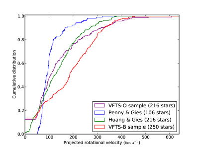
Figure 15: Comparison of the cumulative distribution of projected rotational velocities of our work (VFTS-O sample - purple), Penny & Gies (blue), Huang & Gies (green), and the VFTS-B sample of Dufton et al. (2013) (red).

Figure 15 compares our $\varv_{\rm e}\sin i$ cumulative distribution of the O-type stars in 30 Dor with those from the studies summarized above. For Penny & Gies, we only show the LMC sample (106 stars). From the total sample of Huang & Gies, Fig. 15 presents a sub-sample of 216 stars spanning SpT from O9.5 to B1.5 (see figure 4 of their work). Their higher spectral resolution allowed them to extract lower $\varv_{\rm e}\sin i$ values than is possible for our data set (i.e. $\varv_{\rm e}\sin i$  $\leq$ 40  ${\rm km}\>{\rm s}^{-1}$, see Sect. 3.2). Finally, the VFTS B-type star distribution excludes the 47 late-O stars in common with the present work, to preserve the independency of the two samples.

KP tests indicate that the Penny & Gies and VFTS B-star distributions are statistically different, with a confidence level better than 1%, while the Huang & Gies distribution marginally agrees with our O-star distribution ($p\sim 11$%). The fact that Penny & Gies do not correct for macro-turbulence is a straightforward explanation for the absence of slow rotators in their sample. The other three distributions agree well with respect to the fraction of extremely slow rotators. The fraction of VFTS O- and B-stars below our $\varv_{\rm e}\sin i$ resolution limit (see Sect. 3.6), for instance, is roughly similar.

The distribution of $\varv_{\rm e}\sin i$ of the Penny & Gies sample peaks at the same projected rotational velocity as in our distribution. The lack of stars spinning faster than 300 ${\rm km}\>{\rm s}^{-1}$ in their sample is intriguing, but may result from a selection effect. Indeed the FUSE archives may not be representative of the population of fast rotators in the LMC, as individual observing programs may have focused on stars most suitable for their respective science aims, possibly excluding fast rotators as these are notoriously difficult to analyze.

The similarities between the O-star distribution in 30 Dor and the distribution of late-O and early-B Galactic stars of Huang & Gies suggests a limited influence of metallicity. This is consistent with our expectation that stellar winds do not play a significant role in shaping the rotational velocity distributions in both samples, being dominated by stars less massive than 40 $\mathit{M}_{\odot}$.

The differences with the VFTS B-star sample are striking, and lack a straightforward explanation. The B-type stars show a bi-modal population of very slow rotators and fast rotators, with few stars rotating at rates that are typical for the low-velocity peak seen in the VFTS O-type stars. We return to this issue in Sect. 5.

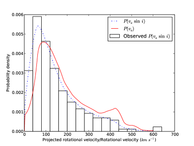
Figure 16: Observed $\varv_{\rm e}\sin i$ and Lucy-deconvolved $\varv_{\rm e}$ distributions. The dot-dashed line shows the estimates, after 4 iterations in the Lucy-deconvolution, of the probability density function for the projected rotational velocity distribution. The solid line shows the probability density function of the actual rotational velocities.

4.5 Analytical representation of the $\varv_{\rm e}$ distribution

The size of our sample is large enough to investigate the distribution of intrinsic rotational velocities. By assuming that the rotation axes are randomly distributed, we infer the probability density function of the rotational velocity distribution $P(\varv_{e})$ from that of $\varv_{\rm e}\sin i$. We adopt the iterative procedure of Lucy (1974), as applied in Paper X for the B-type stars in the VFTS, to estimate the pdf of the projected rotational velocity $\rm{P(\varv_{\rm e}\sin i)}$ and of the corresponding deprojected pdf velocity $\rm{P(\varv_{\rm e})}$. As expected, $\rm{P(\varv_{\rm e})}$ moves to larger velocities compared to $\rm{P(\varv_{\rm e}\sin i)}$ due to the effect of inclination. At $\varv_{\rm e}$ $\geq$ 300 ${\rm km}\>{\rm s}^{-1}$, $\rm{P(\varv_{\rm e})}$ presents small scale fluctuations that probably result from small numbers in the observed distribution. The two extremely fast rotators at $\varv_{\rm e}\sin i$ $\mathrel{\hbox{\hbox to0.0pt{\hbox{\lower 4.0pt\hbox{$\sim$}}\hss}\hbox{$>$}}}$ 600 ${\rm km}\>{\rm s}^{-1}$ are excluded from the deconvolution for numerical stability reasons.

We can well approximate the deconvolved rotational velocity distribution by an analytical function with two components. We use a gamma distribution for the low-velocity peak and a Normal distribution to model the high-velocity contribution:

$$P(\mathrm{v_{e}})\approx I_{\gamma}\ g(\mathrm{v_{e}};\alpha,\beta)+I_{N}\ N(\mathrm{v_{e}};\mu,\sigma^{2})$$ (1)

where

$$g(x;\alpha,\beta) = \frac{\beta^{\alpha}}{\Gamma(\alpha)}x^{\alpha-1}e^{-\beta x},$$ (2)

$$N(x;\mu,\sigma^{2}) = \frac{1}{\sqrt{2\pi}\sigma}e^{-(x-\mu)^{2}/2\sigma^{2}},$$ (3)

and $I_{\gamma}$ and $I_{N}$ are the relative contributions of both distributions to $P(v_{\mathrm{e}})$. The best representation, shown in Fig. 17, is obtained for:

$$P(v_{\mathrm{e}}) \approx 0.43\,g\left(\alpha=4.82,\beta=1/25\right)$$ (4)

$$+ 0.67\,N\left(\mu=205\leavevmode\nobreak\ \mbox{${\rm km}\>{\rm s}^{-1}$},\sigma^{2}=\left(190\leavevmode\nobreak\ \mbox{${\rm km}\>{\rm s}^{-1}$}\right)^{2}\right)$$

The function is normalized to 0.99 to allow for the inclusion of an additional 1% component to represent the two extremely fast rotators is our sample. One should note that the reliability of the fit function is limited by the sample size at extreme rotational velocities. This analytical representation of the intrinsic rotational velocity distribution may be valuable in stellar population synthesis models that account for rotational velocity distributions.

Figure 17: Analytical representation of the deconvolved rotational velocity distribution (Eq. 4).

5 Discussion

The most distinctive feature of the $\varv_{\rm e}\sin i$ and $\varv_{\rm e}$ distributions of the O-type stars in 30 Dor is its two-component structure: a low-velocity peak and an extended high-velocity tail. In this section, we consider possible physical mechanisms that may be responsible for the global shape of our $\varv_{\rm e}$ distribution. We start, however, by assessing the projected spin rates $\varv_{\rm e}\sin i$ relative to the critical spin rates.

5.1 $\varv_{\rm e}\sin i$ relative to the critical rotation rate

To estimate the critical rotation rate, $\varv_{\rm crit}$, the sample is divided into three groups with LC V-IV, III, and II-I. Stellar masses ($M$), luminosities ($L$), and radii ($R$) are then obtained from the SpT calibration for the representative LC (V, III, or I) from the spectral sub-type calibration for rotating LMC stars by Weidner & Vink (2010). We approximate $\varv_{\rm crit}^{2}=\mathrm{G}M(1-\Gamma)/R$ by correcting the mass for the effect of radiation pressure on free electrons with an Eddington factor $\Gamma$. Around 50% of our sample stars are found in the low-velocity peak with $\varv_{\rm e}\sin i$ between 50 and 150 ${\rm km}\>{\rm s}^{-1}$, implying rotation rates less than 20% of the critical rotation rate $\varv_{\rm crit}$. Fig. 18 confirms the general behaviour found in Sect. 4.3 that earlier O-type stars in our sample lack extremely fast rotators relative to later spectral sub-types, either in absolute $\varv_{\rm e}\sin i$ or as a fraction of $\varv_{\rm crit}$.

5.2 The low-velocity peak

The low-velocity peak contains the large majority of the stars in our sample. The origin of this peak may be related to the formation or early evolution of these stars. Massive stars inherit their angular momentum from their parental cloud that contains more than sufficient angular momentum to spin up the proto-star to critical rotation (see Larson, 2010). Interestingly, Lin et al. (2011) found that gravitational torques prohibit a star from rotating above $\sim$50% of its break-up speed during formation. Magnetic coupling between the massive proto-star and its accretion disk is expected to be insufficient in spinning down the star further (Rosen et al., 2012). As pointed out earlier, stellar winds and (single-star) evolution are also not effective in reducing the rotation rate during most of the main sequence phase, save for objects initially more massive than 40 $\mathit{M}_{\odot}$. An additional braking mechanism is thus needed.

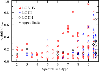
Figure 18: Projected rotational velocity normalized to critical velocity, $\varv_{\rm e}\sin i$$/\rm{v_{crit}}$, vs. spectral sub-type for our sample stars with known spectral types. Critical velocities are estimated using the SpT calibration by Weidner & Vink. See legend for the information on the luminosity class. Stars indicated in the legend as “upper limits” refer to stars with $\varv_{\rm e}\sin i$ $\leq$ 40  ${\rm km}\>{\rm s}^{-1}$.

Meynet et al. (2011) and Potter et al. (2012) have explored stellar evolution models for magnetic main sequence stars. Based on a model for magnetic braking of ud-Doula & Owocki (2002), they both predict that a massive star rotates at only a modest fraction of its break-up velocity if it has a surface magnetic field strength of the order of 2 kG. Most O-type stars in the Milky Way have no measured magnetic field and the majority of the few known magnetic O-type star have a magnetic field strength of the order of several hundreds of G to a couple of kG (Donati & Landstreet, 2009; Grunhut et al., 2012). If magnetic braking is indeed the mechanism that slows down the stars after their birth, most of the spin down has to occur within the first Myr, after which the strength of the stellar magnetic field has to decrease below the detection limit of the current surveys.

Within the context of a main-sequence magnetic braking scenario, the absence of a large population of very slow rotators ($\varv_{\rm e}\sin i$ $<$ 40 ${\rm km}\>{\rm s}^{-1}$) in our sample may indicate that either magnetic fields disappear before being able to fully spin down the star or that the generation of the magnetic field itself is related to the high rotational velocity. The analysis of spin rates for the early-B stars in the VFTS field (Paper X) shows a bi-modal distribution with a low-velocity component that peaks at lower velocities relative to that for the O-stars. If this difference is connected to magnetic braking it may indicate that magnetic fields are initially stronger and/or more efficient in spinning down early-B stars.

5.3 The high-velocity tail

Although most of the stars must spin down quickly after their formation in order to produce the low-velocity peak (see Sect. 5.2), it is possible that some very young stars – potentially rotating faster than average – are still present in our sample. Fig. 18 shows that the later spectral sub-types contain a pro rata larger percentage of fast rotating stars, almost reaching up to critical speed. The compatible rotational distributions of the stars in NGC 2060 and the younger NGC 2070 (see Sect. 4.1) and the fact that star formation has likely stopped in NGC 2060, however, argue against newborn stars being a suitable explanation for the high-velocity tail.

The presence of a high-velocity tail is, however, predicted by recent population synthesis computations that study the influence of binary evolution on the projected rotation rate of massive stars (de Mink et al., 2013). Those simulations can create a population of stars with high rotational rates through binary interaction. Such a population is composed of mergers and of secondary stars that have been spun up by mass transfer. In a second paper, de Mink et al. (in prep.) also argue that most post-interaction binary products cannot be identified by RV investigations and will thus contaminate our “single-star” sample. Interestingly, we find that the fraction of fast rotators ($\varv_{\rm e}$ $>$ 300 ${\rm km}\>{\rm s}^{-1}$) observed in the 30 Dor O-type star population (19% of our ‘single-star’ sample, hence $\sim$11% of the whole VFTS O-type star population) is of the same order of magnitude as the numerical predictions by de Mink et al. Dedicated simulations that take into account the star formation history of 30 Dor are, however, desirable to further investigate this scenario. Sana et al. (2013; Paper VIII) report that the measured O-type star binary fraction in 30 Dor (51%) is apparently smaller than this fraction measured in young nearby Milky Way clusters (69%; Sana et al., 2012). The assumption that most of the stars in our high rotational-velocity tail are post-binary interaction products could potentially conciliate these two measurements. The pronounced high-velocity component in the $\varv_{\rm e}\sin i$ distribution of the early-B stars in the VFTS (Paper X) may also be in line with a post-binary nature, as secondaries more often are of spectral type B than O.

If our interpretation of the high-velocity tail as resulting from binary interaction is correct, it suggests that the low-velocity part of our distribution is a cleaner original single-star sample. As discussed by de Mink et al. (2013) the contamination of the high-velocity end of the distribution by unresolved binary products complicates, and may even invalidate, surface abundance analysis aiming to test or calibrate rotational mixing theories, as such surface enrichment may also be the result of mass transfer or mixing in merger products.

5.4 The single and binary channel for long-duration gamma-ray bursts

The nature of the high-velocity tail of the distribution of rotation rates as discussed in Sect. 5.3 has important implications for the evolutionary origin of systems that produce long-duration gamma-ray bursts (LGRBs). In both the collapsar model (Woosley, 1993) and the millisecond-magnetar model (Lyutikov & Blackman, 2001) the Wolf-Rayet progenitor system of a stellar explosion producing a long (at least two second) burst of gamma rays is required to have a rapidly spinning core (see e.g. Langer, 2012). Most, perhaps all (Niino, 2011), of such gamma-ray bursts occur in regions of their host galaxies that have a low-metal content (Fruchter et al., 2006; Modjaz et al., 2008; Gräfener & Hamann, 2008). Two channels leading up to a GRB have been proposed. First, a close interacting binary system may lead to the late production and spin-up of a Wolf-Rayet star (Izzard et al., 2004; Fryer & Heger, 2005; Podsiadlowski et al., 2010; Tout et al., 2011). With only limited time left before the supernova explosion, the stellar wind of the Wolf-Rayet is not able to remove sufficient angular momentum to prevent a gamma-ray burst, especially not at low-metallicity where the outflow is less dense (Vink & de Koter, 2005). Second, a LGRB may occur for a single star that rotates so fast that mixing processes cause the interior to become quasi-chemically homogeneous and the star as a whole to remain compact (Yoon & Langer, 2005; Woosley & Heger, 2006). As such a system develops Wolf-Rayet characteristics early on, a low-metallicity environment is required to avoid wind-induced spin down.

The single-star LGRB progenitors need O-type star descendants that at birth spin faster than $\sim$ 300-400 ${\rm km}\>{\rm s}^{-1}$ and are more massive than about 20 $\mathit{M}_{\odot}$ (Brott et al., 2011a). Mokiem et al. (2006) identified presumably-single candidate objects for such evolution, a result that actually spurred the above mentioned groups to put forward the possibility of a single-star channel. If indeed the high-end tail of the velocity distribution is dominated by, or is exclusively due to, post-interaction binaries and mergers, the relative importance of the single-star channel is reduced. Indeed, if the high-end tail is exclusively composed of binary products then the existence of the single-star GRB channel may be challenged altogether.

6 Conclusions

We have estimated projected rotational velocities for the presumably single O-type stars in the VFTS sample (216 stars). We find that the most distinctive feature of the $\varv_{\rm e}\sin i$ distribution of O stars in 30 Dor is a two-component structure: a low-velocity peak at $\sim$80 ${\rm km}\>{\rm s}^{-1}$ and a high-velocity tail extending up to $\sim$600 ${\rm km}\>{\rm s}^{-1}$. The presence of the low-velocity peak is consistent with previous LMC surveys, but we conclusively find a considerable population of rapidly spinning stars ($\varv_{\rm e}$ $>$ 300 ${\rm km}\>{\rm s}^{-1}$ for 20% of the sample). The homogeneity and size of the sample also allows us to study the $\varv_{\rm e}\sin i$ distribution as a function of spatial distribution, luminosity class and spectral type.

Based on expectations of star-formation and single-star evolution, most of the stars seem to have to spin down shortly after their formation, from critical or half-critical rotation rates to a much smaller fraction of their break-up velocity. For the bulk of O stars angular momentum loss in a stellar wind is insufficient and another mechanism should act to efficiently spin down the stars; magnetic fields being prime candidates.

The presence of a well populated high-velocity tail is compatible with expectations from binary evolution and qualitatively agrees with recent population synthesis predictions (de Mink et al., 2013). The nature of the high-velocity tail of the distribution has an important implication for the evolutionary origin of systems that produce long-duration gamma-ray bursts. If the objects in the high-velocity tail are predominantly products of binary interaction and mergers this would imply a scenario for long-duration GRB production without a preferred metallicity (range) for the progenitor systems, unless binarity itself presents a metallicity dependence in LGRB progenitor production. If the high-velocity tail is dominated by single stars after all, a low metallicity environment seems required for LGRBs.

Appendix A N v $\lambda$4604 line

Though the N v line is not widely used to obtain $\varv_{\rm e}\sin i$, the line is little affected by Stark broadening and may thus provide an alternative anchor point for He ii-based measurements. As N v $\lambda$4604 is intrinsically strong it may be partly formed in the stellar outflow. It can thus only be used for $\varv_{\rm e}\sin i$ determination if the wind is weak and the line is of photospheric origin, i.e. it should be symmetric.

Eight stars in our sample (VFTS 016, 072, 180, 267, 506, 518, 566, 599, 621) show both N v $\lambda$4604 and He ii $\rm{\lambda}$4541.VFTS 180 was discarded due to its asymmetric profile. Fig. 19 compares the $\varv_{\rm e}\sin i$ measurements obtained, for the remainder sample, from both diagnostic lines. Save for one target, all measurements agree within $\pm 10$ ${\rm km}\>{\rm s}^{-1}$ and/or $\pm\,10$% of the 1:1 relation. The comparison lacks stars with low projected spin rates. The sole case for which the comparison is poor has the lowest spin rate when using the N v diagnostic. On the basis of one case we cannot conclude whether this indicates a systematic effect at low $\varv_{\rm e}\sin i$ or whether it is the result of the relatively large dispersion of spin rate measurements based on He ii at modest rotational velocities (see Sect. 3.4.2).

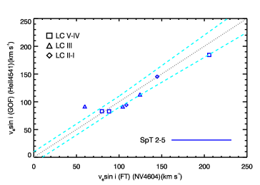
Figure 19: Comparison of the $\varv_{\rm e}\sin i$ measurements for He ii $\rm{\lambda}$4541 and N v $\lambda$4604. Information on the LC of the targets is provided by the symbol shapes. The dashed lines show the $\pm 10$ ${\rm km}\>{\rm s}^{-1}$ and/or $\pm\,10$%, whichever is the largest, around the 1:1 relation.

Appendix B Comparison with overlapping sample of the O and B-type stars in the VFTS

Rotational velocities for the single B-type stars in the Tarantula Survey have been presented in Paper X. There the FT technique was also used, but a different set of lines was applied reflecting the different temperature range. Due to uncertainties in the preliminary spectral classification, 47 late-O and early-B stars were included in both data sets.

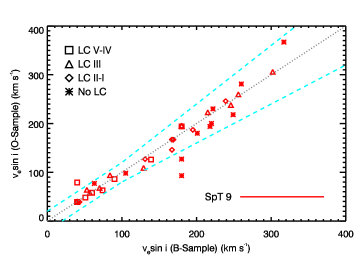
Figure 20: Comparison of the $\varv_{\rm e}\sin i$ measurements of the overlapping late O-type sample in Dufton et al. (2013) and this study. Information on the LC of the targets is provided by the symbol shapes. The dashed and dotted lines have the same meaning as in Fig. 6.

Fig. 20 compares both $\varv_{\rm e}\sin i$ measurements. We find that there are no significant systematic differences between the two sets of measurements. Despite two outliers (VFTS 412 and 594 at about $\sim$180 ${\rm km}\>{\rm s}^{-1}$), the overall comparison presents an excellent agreement, with a rms dispersion of about 10% of the 1:1 relation.