Quantum theory of photonic crystals

Abstract

In this paper, we have firstly presented a new quantum theory to study one-dimensional photonic crystals. We give the quantum transform matrix, quantum dispersion relation and quantum transmissivity, and compare them with the classical dispersion relation and classical transmissivity. By the calculation, we find the classical and quantum dispersion relation and transmissivity are identical. The new approach can be studied two-dimensional and three-dimensional photonic crystals.

PACS: 42.70.Qs, 78.20.Ci, 41.20.Jb
Keywords: Photonic crystals; Quantum transmissivity; Quantum dispersion relation

1. Introduction

Photonic crystals (PCs) are artificial materials with periodic variations in refractive index that are designed to affect the propagation of light [1-4]. An important feature of the PCs is that there are allowed and forbidden ranges of frequencies at which light propagates in the direction of index periodicity. Due to the forbidden frequency range, known as photonic band gap (PBG) [5-6], which forbids the radiation propagation in a specific range of frequencies. The existence of PBGs will lead to many interesting phenomena. In the past ten years has been developed an intensive effort to study and micro-fabricate PBG materials in one, two or three dimensions, e.g., modification of spontaneous emission [7-9] and photon localization [10-14].

Thus numerous applications of PCs have been proposed in improving the performance of optoelectronic and microwave devices such as high-efficiency semiconductor lasers, right emitting diodes, wave guides, optical filters, high-Q resonators, antennas, frequency-selective surface, optical wave guides and sharp bends [15], WDM-devices [16-17], splitters and combiners [18]. optical limiters and amplifiers [19-20].

At present, the theory calculations of PCs have many numerical methods, such as: the plane-wave expansion method (PWE) [21-23], the finite-difference time-domain method (FDTD) [24-27], the transfer matrix method (TMM) [28-29], the finite element method (FE) [30-33], the scattering matrix method [34], the Green’s function method [35] and so on. These methods are classical electromagnetism theory. Obviously, the full quantum theory of PCs is necessary. In Refs. [36-37], the authors give the quantum wave equation of single photon. In Ref. [38], we give the quantum wave equations of free and non-free photon. In this paper, We have studied the 1D PCs by the quantum wave equations of photon [38], and give quantum dispersion relation, quantum transmissivity and reflectivity, and obtain some new results, which can be tested by experiments. Obviously, the new method of quantum theory can be studied the 2D and 3D PCs.

2. The quantum wave equation and probability current density of photon

The quantum wave equations of free and non-free photon have been obtained in Ref. [39], they are

$$i\hbar\frac{\partial}{\partial t}\vec{\psi}(\vec{r},t)=c\hbar\nabla\times\vec{\psi}(\vec{r},t),$$ (1)

and

$$i\hbar\frac{\partial}{\partial t}\vec{\psi}(\vec{r},t)=c\hbar\nabla\times\vec{\psi}(\vec{r},t)+V\vec{\psi}(\vec{r},t),$$ (2)

where $\vec{\psi}(\vec{r},t)$ is the vector wave function of photon, and $V$ is the potential energy of photon in medium. In the medium of refractive index $n$, the photon’s potential energy $V$ is [39]

$$V=\hbar\omega(1-n).$$ (3)

The conjugate of Eq. (2) is

$$-i\hbar\frac{\partial}{\partial t}\vec{\psi}^{\ast}(\vec{r},t)=c\hbar\nabla\times\vec{\psi}^{\ast}(\vec{r},t)+V\vec{\psi}^{\ast}(\vec{r},t).$$ (4)

Multiplying the Eq. (2) by $\vec{\psi}^{\ast}$, the Eq. (4) by $\vec{\psi}$, and taking the difference, we get

$$i\hbar\frac{\partial}{\partial t}(\vec{\psi}^{\ast}\cdot\vec{\psi})=c\hbar(\vec{\psi}^{\ast}\cdot\nabla\times\vec{\psi}-\vec{\psi}\cdot\nabla\times\vec{\psi}^{\ast})=c\hbar\nabla\cdot(\vec{\psi}\times\vec{\psi}^{\ast}),$$ (5)

i.e.

$$\frac{\partial\rho}{\partial t}+\nabla\cdot J=0,$$ (6)

where

$$\rho=\vec{\psi}^{\ast}\cdot\vec{\psi},$$ (7)

and

$$J=ic\vec{\psi}\times\vec{\psi}^{\ast},$$ (8)

are the probability density and probability current density, respectively.

By the method of separation variable

$$\vec{\psi}(\vec{r},t)=\vec{\psi}(\vec{r})f(t),$$ (9)

the time-dependent Eq. (2) becomes the time-independent equation

$$c\hbar\nabla\times\vec{\psi}(\vec{r})+V\vec{\psi}(\vec{r})=E\vec{\psi}(\vec{r}),$$ (10)

where $E$ is the energy of photon in medium.

By taking curl in (10), when $\frac{\partial V}{\partial x_{i}}=0,(i=1,2,3)$, the Eq. (10) becomes

$$(\hbar c)^{2}(\nabla(\nabla\cdot\vec{\psi}(\vec{r}))-\nabla^{2}\vec{\psi}(\vec{r}))=(E-V)^{2}\vec{\psi}(\vec{r}).$$ (11)

Choosing transverse gange $\nabla\cdot\vec{\psi}(\vec{r})=0$, Eq. (11) becomes

$$\nabla^{2}\vec{\psi}(\vec{r})+(\frac{E-V}{\hbar c})^{2}\vec{\psi}(\vec{r})=0.$$ (12)

In vacuum, potential energy $V=0$, Eq. (12) becomes

$$\nabla^{2}\vec{\psi}(\vec{r})+K^{2}\vec{\psi}(\vec{r})=0.$$ (13)

Where $K=\frac{\omega}{c}$. Eqs. (12) and (13) are the quantum wave equation of photon in medium and vacuum, and we can study one-dimensional PCs by them.

3. The quantum theory of one-dimensional Photonic crystals

For one-dimensional Photonic crystals, we should define and calculate its quantum dispersion relation and quantum transmissivity. The one-dimensional PCs structure is shown in FIG. 1.

In FIG. 1, $\vec{\psi}_{I}$, $\vec{\psi}_{R}$, $\vec{\psi}_{T}$ are the wave functions of incident, reflection and transmission photon, respectively. By Eq. (13), they can be written as

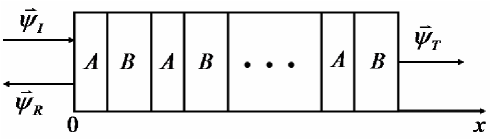
Figure 1: the structure of one-dimensional photonic crystals

$$\vec{\psi}(\vec{r},t) = \vec{\psi}_{0}e^{i(\vec{K}\cdot\vec{r}-\omega t)}=\psi_{x}\vec{i}+\psi_{y}\vec{j}+\psi_{z}\vec{k}$$ (14)

$$= \psi_{x0}e^{i(\vec{K}\cdot\vec{r}-\omega t)}\vec{i}+\psi_{y0}e^{i(\vec{K}\cdot\vec{r}-\omega t)}\vec{j}+\psi_{z0}e^{i(\vec{K}\cdot\vec{r}-\omega t)}\vec{k},$$

By transverse gange $\nabla\cdot\vec{\psi}(\vec{r})=0$, we get

$$K_{x}\psi_{x}+K_{y}\psi_{y}+K_{z}\psi_{z}=0.$$ (15)

In FIG. 1, the photon travels along with the $x$ axis, the wave vector $K_{y}=K_{z}=0$ and $K_{x}\neq 0$. By Eq. (15), we have

$$\psi_{x}=0,$$ (16)

so the total wave function of photon is

$$\vec{\psi}=\vec{\psi}_{y}\vec{j}+\vec{\psi}_{z}\vec{k}.$$ (17)

By the wave function continuum, the $\psi_{x}=0$ in medium. So, the Eq. (13) becomes two component equations

$$\nabla^{2}\psi_{y}+(\frac{E-V}{\hbar c})^{2}\psi_{y}=0,$$ (18)

and

$$\nabla^{2}\psi_{z}+(\frac{E-V}{\hbar c})^{2}\psi_{z}=0.$$ (19)

In FIG. 1, the wave functions of incident, reflection and transmission photon can be written as

$$\vec{\psi_{I}}=F_{y}e^{i(\vec{K}\cdot\vec{r}-\omega t)}\vec{j}+F_{z}e^{i(\vec{K}\cdot\vec{r}-\omega t)}\vec{k},$$ (20)

$$\vec{\psi_{R}}=F_{y}^{{}^{\prime}}e^{-i(\vec{K}\cdot\vec{r}+\omega t)}\vec{j}+F_{z}^{{}^{\prime}}e^{-i(\vec{K}\cdot\vec{r}+\omega t)}\vec{k},$$ (21)

$$\vec{\psi_{T}}=D_{y}e^{i(\vec{K}\cdot\vec{r}-\omega t)}\vec{j}+D_{z}e^{i(\vec{K}\cdot\vec{r}-\omega t)}\vec{k},$$ (22)

where $F_{y}$, $F_{z}$, $F_{y}^{{}^{\prime}}$, $F_{z}^{{}^{\prime}}$, $D_{y}$, and $D_{z}$ are their amplitudes.

The component form of Eq. (1) is

$$\left\{\begin{array}[]{lll}&&i\hbar\frac{\partial}{\partial t}\psi_{x}=\hbar c(\frac{\partial\psi_{z}}{\partial y}-\frac{\partial\psi_{y}}{\partial z})\\ &&i\hbar\frac{\partial}{\partial t}\psi_{y}=\hbar c(\frac{\partial\psi_{x}}{\partial z}-\frac{\partial\psi_{z}}{\partial x})\\ &&i\hbar\frac{\partial}{\partial t}\psi_{z}=\hbar c(\frac{\partial\psi_{y}}{\partial x}-\frac{\partial\psi_{x}}{\partial y})\end{array}\right.,$$ (26)

substituting Eqs. (14) and (16) into (23), we have

$$\psi_{z}=i\psi_{y},$$ (27)

the probability current density becomes

$$J=ic\vec{\psi}\times\vec{\psi}^{\ast}=2c|\psi_{z}|^{2}\vec{i}=2c|\psi_{0z}|^{2}\vec{i},$$ (28)

where

$$\psi_{z}=\psi_{0z}e^{i(\vec{k}\cdot\vec{r}-\omega t)},$$ (29)

the $\psi_{0z}$ is $\psi_{z}$ amplitude.

For the incident,reflection and transmission photon, their probability current density $J_{I}$, $J_{R}$, $J_{T}$ are

$$J_{I}=2c|F_{z}|^{2},$$ (30)

$$J_{R}=2c|F_{z}^{{}^{\prime}}|^{2},$$ (31)

$$J_{T}=2c|D_{z}|^{2},$$ (32)

We can define quantum transmissivity $T$ and quantum reflectivity $R$ as

$$T=\frac{J_{T}}{J_{I}}=|\frac{D_{z}}{F_{z}}|^{2},$$ (33)

$$R=\frac{J_{R}}{J_{I}}=|\frac{F^{\prime}_{z}}{F_{z}}|^{2}.$$ (34)

With Eqs. (30) and (31), we find quantum transmissivity and reflectivity are relevant to the $z$ component amplitudes of wave function of the incident, reflection and transmission photon.

4. The quantum transmissivity and quantum dispersion relation

Since the quantum transmissivity is relevant to the $z$ component amplitude of transmission wave function, we should only solve the $z$ component equation (19) for the one-dimensional PCs, which is shown in FIG. 2

Figure 2: the structure of one-dimensional photonic crystals

With Eq. (19), the photon’s quantum wave equation in mediums $A$ and $B$ are

$$\frac{\partial^{2}\psi_{A}}{\partial x^{2}}+k_{A}^{2}\psi_{A}=0\hskip 43.36243pt(0<x<a),$$ (35)

$$\frac{\partial^{2}\psi_{B}}{\partial x^{2}}+k_{B}^{2}\psi_{B}=0\hskip 43.36243pt(a<x<a+b),$$ (36)

where

$$k_{A}=\frac{E-V_{a}}{\hbar c}=\frac{E-\hbar\omega(1-n_{a})}{\hbar c}=\frac{\omega}{c}n_{a}=\frac{2\pi}{\lambda}n_{a},$$ (37)

$$k_{B}=\frac{E-V_{b}}{\hbar c}=\frac{E-\hbar\omega(1-n_{b})}{\hbar c}=\frac{\omega}{c}n_{b}=\frac{2\pi}{\lambda}n_{b},$$ (38)

where $\lambda={2\pi c}/{\omega}$ is the photon wave length in vacuum, $V_{a}=\hbar\omega(1-n_{a})\hskip 3.61371pt(V_{b}=\hbar\omega(1-n_{b}))$ is the potential energy of photon in medium $A(B)$, and $n_{a}(n_{b})$ is refractive index of medium $A(B)$. In order to simplify, the index $z$ is omitted, i.e., $\psi_{zA}(\psi_{zB})$ is written as $\psi_{A}(\psi_{B})$.
The solutions of Eqs. (32) and (33) are

$${\psi_{A}}=A_{1}e^{ik_{A}x}+A_{2}e^{-ik_{A}x}\hskip 43.36243pt(0<x<a),$$ (39)

$${\psi_{B}}=B_{1}e^{ik_{B}x}+B_{2}e^{-ik_{B}x}\hskip 43.36243pt(a<x<a+b).$$ (40)

By Bloch law, there is

$${\psi(a+b<x<2a+b)} = \psi(0<x<a)e^{ik(a+b)}$$ (41)

$$= (A_{1}e^{ik_{A}(x-(a+b))}$$

$$+A_{2}e^{-ik_{A}(x-(a+b))})e^{ik(a+b)},$$

where $k$ is Bloch wave vector.
At $x=a$, by the continuation of wave function and its derivative, we have

$$A_{1}e^{ik_{A}a}+A_{2}e^{-ik_{A}a}=B_{1}e^{ik_{B}a}+B_{2}e^{-ik_{B}a},$$ (42)

$$ik_{A}A_{1}e^{ik_{A}a}-ik_{A}A_{2}e^{-ik_{A}a}=ik_{B}B_{1}e^{ik_{B}a}-ik_{B}B_{2}e^{-ik_{B}a},$$ (43)

At $x=a+b$, by the continuation of wave function and its derivative, we have

$$A_{1}e^{ik(a+b)}+A_{2}e^{ik(a+b)}=B_{1}e^{ik_{B}(a+b)}+B_{2}e^{-ik_{B}(a+b)},$$ (44)

$$ik_{A}A_{1}e^{ik(a+b)}-ik_{A}A_{2}e^{ik(a+b)}=ik_{B}B_{1}e^{ik_{B}(a+b)}-ik_{B}B_{2}e^{-ik_{B}(a+b)},$$ (45)

and we obtain the follows equations set

$$\left\{\begin{array}[]{ll}A_{1}e^{ik_{A}a}+A_{2}e^{-ik_{A}a}=B_{1}e^{ik_{B}a}+B_{2}e^{-ik_{B}a}\\ ik_{A}A_{1}e^{ik_{A}a}-ik_{A}A_{2}e^{-ik_{A}a}=ik_{B}B_{1}e^{ik_{B}a}-ik_{B}B_{2}e^{-ik_{B}a}\\ A_{1}e^{ik(a+b)}+A_{2}e^{ik(a+b)}=B_{1}e^{ik_{B}(a+b)}+B_{2}e^{-ik_{B}(a+b)}\\ ik_{A}A_{1}e^{ik(a+b)}-ik_{A}A_{2}e^{ik(a+b)}=ik_{B}B_{1}e^{ik_{B}(a+b)}-ik_{B}B_{2}e^{-ik_{B}(a+b)},\\ \end{array}\right.$$ (50)

the necessary and sufficient condition of Eq. (43) nonzero solution is its coefficient determinant equal to zero

$$\left|\begin{array}[]{llll}\hskip 14.45377pte^{ik_{A}a}\hskip 43.36243pte^{-ik_{A}a}\hskip 43.36243pt-e^{ik_{B}a}\hskip 36.135pt-e^{-ik_{B}a}\\ \hskip 14.45377ptk_{A}e^{ik_{A}a}\hskip 28.90755pt-k_{A}e^{-ik_{A}a}\hskip 21.68121pt-k_{B}e^{ik_{B}a}\hskip 28.90755ptk_{B}e^{-ik_{B}a}\\ \hskip 14.45377pte^{ik(a+b)}\hskip 28.90755pte^{ik(a+b)}\hskip 43.36243pt-e^{ik_{B}(a+b)}\hskip 21.68121pt-e^{-ik_{B}(a+b)}\\ \hskip 14.45377ptk_{A}e^{ik(a+b)}\hskip 14.45377pt-k_{A}e^{ik(a+b)}\hskip 21.68121pt-k_{B}e^{ik_{B}(a+b)}\hskip 14.45377ptk_{B}e^{-ik_{B}(a+b)}\\ \end{array}\right|=0,$$ (55)

simplifying Eq. (44), we obtain the quantum dispersion relation

$$\cos(k(a+b))=\cos(k_{A}a)\cos(k_{B}b)-\frac{1}{2}(\frac{1}{k_{A}}+\frac{1}{k_{B}})\sin(k_{A}a)\sin(k_{B}b).$$ (56)

In the following, we should give the wave function of photon in every medium, and the transmission wave function. In FIG. 3, we give the simplification form of wave function in every medium, such as symbols $A_{k_{A}}^{1}$ and $A_{-k_{A}}^{1}$ express simplifying wave function of medium $A$ in the first period, it express wave function

$${\psi_{A^{1}}(x)}=A_{k_{A}}^{1}e^{ik_{A}x}+A_{-k_{A}}^{1}e^{-ik_{A}x},$$ (57)

in medium $B$ of first period, the symbols $B_{k_{A}}^{1}$ and $B_{-k_{A}}^{1}$ express wave function

$${\psi_{B^{1}}(x)}=B_{k_{B}}^{1}e^{ik_{B}x}+B_{-k_{B}}^{1}e^{-ik_{B}x},$$ (58)

in medium $A$ of second period, the symbols $A_{k_{A}}^{2}$ and $A_{-k_{A}}^{2}$ express wave function

$${\psi_{A^{2}}(x)}=A_{k_{A}}^{2}e^{ik_{A}x}+A_{-k_{A}}^{2}e^{-ik_{A}x},$$ (59)

similarly, in medium $B$ of second period, the symbols $B_{k_{A}}^{2}$ and $B_{-k_{A}}^{2}$ express wave function

$${\psi_{B^{2}}(x)}=B_{k_{B}}^{2}e^{ik_{B}x}+B_{-k_{B}}^{2}e^{-ik_{B}x},$$ (60)

and so on.
In the incident area, the total wave function $\psi_{tot}(x)$ is the superposition of incident and reflection wave function, it is

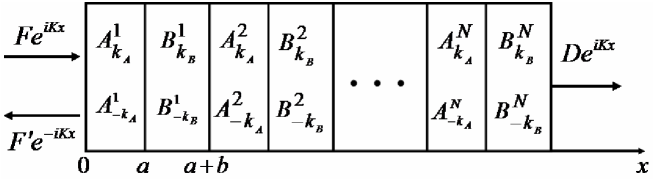
Figure 3: the quantum structure of one-dimensional photonic crystals

$${\psi_{tot}(x)}={\psi_{I}(x)}+{\psi_{R}(x)}=Fe^{iKx}+F^{\prime}e^{-iKx},$$ (61)

where $K$ is the wave vector of incident, reflection, and transmission photon. In the following, we should use the condition of wave function and its derivative continuation at interface of two mediums.
(1) At $x=0$, by the continuation of wave function and its derivative, we have

$$F+F^{\prime}=A_{k_{A}}^{1}+A_{-k_{A}}^{1},$$ (62)

$$iKF-iKF^{\prime}=ik_{A}A_{k_{A}}^{1}-ik_{A}A_{-k_{A}}^{1},$$ (63)

we obtain

$$A_{k_{A}}^{1}=\frac{1}{2}[(1+\frac{K}{k_{A}})F+(1-\frac{K}{k_{A}})F^{\prime}],$$ (64)

$$A_{-k_{A}}^{1}=\frac{1}{2}[(1-\frac{K}{k_{A}})F+(1+\frac{K}{k_{A}})F^{\prime}],$$ (65)

the Eqs. (53) and (54) can be written as matrix form

$$\left(\begin{array}[]{ll}A_{k_{A}}^{1}\\ A_{-k_{A}}^{1}\\ \end{array}\right)=\frac{1}{2}\left(\begin{array}[]{ll}1+{K}/{k_{A}}\hskip 14.45377pt1-{K}/{k_{A}}\\ 1-{K}/{k_{A}}\hskip 14.45377pt1+{K}/{k_{A}}\\ \end{array}\right)\left(\begin{array}[]{ll}F\\ F^{\prime}\\ \end{array}\right)=M_{A}^{1}\left(\begin{array}[]{ll}F\\ F^{\prime}\\ \end{array}\right),$$ (74)

where $M_{A}^{1}$ is the quantum transform matrix of the first period medium $A$, it is

$$M_{A}^{1}=\frac{1}{2}\left(\begin{array}[]{ll}1+{K}/{k_{A}}\hskip 14.45377pt1-{K}/{k_{A}}\\ 1-{K}/{k_{A}}\hskip 14.45377pt1+{K}/{k_{A}}\\ \end{array}\right),$$ (77)

(2) At $x=a$, by the continuation of wave function and its derivative, we have

$$A_{k_{A}}^{1}e^{ik_{A}a}+A_{-k_{A}}^{1}e^{-ik_{A}a}=B_{k_{B}}^{1}e^{ik_{B}a}+B_{-k_{B}}^{1}e^{-ik_{B}a},$$ (78)

$$\frac{k_{A}}{k_{B}}(A_{k_{A}}^{1}e^{ik_{A}a}-A_{-k_{A}}^{1}e^{-ik_{A}a})=B_{k_{B}}^{1}e^{ik_{B}a}-B_{-k_{B}}^{1}e^{-ik_{B}a},$$ (79)

we get

$$B_{k_{B}}^{1}=\frac{1}{2}e^{i(k_{A}-k_{B})a}(1+\frac{k_{A}}{k_{B}})A_{k_{A}}^{1}+\frac{1}{2}e^{-i(k_{A}+k_{B})a}(1-\frac{k_{A}}{k_{B}})A_{-k_{A}}^{1},$$ (80)

$$B_{-k_{B}}^{1}=\frac{1}{2}e^{i(k_{A}+k_{B})a}(1-\frac{k_{A}}{k_{B}})A_{k_{A}}^{1}+\frac{1}{2}e^{i(k_{B}-k_{A})a}(1+\frac{k_{A}}{k_{B}})A_{-k_{A}}^{1},$$ (81)

the Eqs. (59) and (60) can be written as matrix form

$$\left(\begin{array}[]{ll}B_{k_{B}}^{1}\\ B_{-k_{B}}^{1}\\ \end{array}\right)=\frac{1}{2}\left(\begin{array}[]{ll}e^{i(k_{A}-k_{B})a}(1+{k_{A}}/{k_{B}})\hskip 14.45377pte^{-i(k_{A}+k_{B})a}(1-{k_{A}}/{k_{B}})\\ e^{i(k_{A}+k_{B})a}(1-{k_{A}}/{k_{B}})\hskip 14.45377pte^{i(k_{B}-k_{A})a}(1+{k_{A}}/{k_{B}})\\ \end{array}\right)\left(\begin{array}[]{ll}A_{kA}^{1}\\ A_{-kA}^{1}\\ \end{array}\right)=M_{B}^{1}\left(\begin{array}[]{ll}A_{kA}^{1}\\ A_{-kA}^{1}\\ \end{array}\right),$$ (90)

where $M_{B}^{1}$ is the quantum transform matrix of the first period medium $B$, it is

$$M_{B}^{1}=\frac{1}{2}\left(\begin{array}[]{ll}e^{i(k_{A}-k_{B})a}(1+{k_{A}}/{k_{B}})\hskip 14.45377pte^{-i(k_{A}+k_{B})a}(1-{k_{A}}/{k_{B}})\\ e^{i(k_{A}+k_{B})a}(1-{k_{A}}/{k_{B}})\hskip 14.45377pte^{i(k_{B}-k_{A})a}(1+{k_{A}}/{k_{B}})\\ \end{array}\right),$$ (93)

(3) At $x=a+b$, by the continuation of wave function and its derivative, we have

$$B_{k_{B}}^{1}e^{ik_{B}(a+b)}+B_{-k_{B}}^{1}e^{-ik_{B}(a+b)}=A_{k_{A}}^{2}e^{ik_{A}(a+b)}+A_{-k_{A}}^{2}e^{-ik_{A}(a+b)},$$ (94)

$$\frac{k_{B}}{k_{A}}(B_{k_{B}}^{1}e^{ik_{B}(a+b)}-B_{-k_{B}}^{1}e^{-ik_{B}(a+b)})=A_{k_{A}}^{2}e^{ik_{A}(a+b)}-A_{-k_{A}}^{2}e^{-ik_{A}(a+b)},$$ (95)

we get

$$A_{k_{A}}^{2}=\frac{1}{2}e^{i(k_{B}-k_{A})(a+b)}(1+\frac{k_{B}}{k_{A}})B_{k_{B}}^{1}+\frac{1}{2}e^{-i(k_{A}+k_{B})(a+b)}(1-\frac{k_{B}}{k_{A}})B_{-k_{B}}^{1},$$ (96)

$$A_{-k_{A}}^{2}=\frac{1}{2}e^{i(k_{A}+k_{B})(a+b)}(1-\frac{k_{B}}{k_{A}})B_{k_{B}}^{1}+\frac{1}{2}e^{i(k_{A}-k_{B})(a+b)}(1+\frac{k_{B}}{k_{A}})B_{-k_{B}}^{1},$$ (97)

the Eqs. (65) and (66) can be written as matrix form

$$\left(\begin{array}[]{ll}A_{k_{A}}^{2}\\ A_{-k_{A}}^{2}\\ \end{array}\right) = \frac{1}{2}\left(\begin{array}[]{ll}e^{i(k_{B}-k_{A})(a+b)}(1+{k_{B}}/{k_{A}})\hskip 7.22743pte^{-i(k_{A}+k_{B})(a+b)}(1-{k_{B}}/{k_{A}})\\ e^{i(k_{A}+k_{B})(a+b)}(1-{k_{B}}/{k_{A}})\hskip 7.22743pte^{i(k_{A}-k_{B})(a+b)}(1+{k_{B}}/{k_{A}})\\ \end{array}\right)\left(\begin{array}[]{ll}B_{kB}^{1}\\ B_{-kB}^{1}\\ \end{array}\right)$$ (104)

$$= M_{A}^{2}\left(\begin{array}[]{ll}B_{kB}^{1}\\ B_{-kB}^{1}\\ \end{array}\right),$$ (107)

where $M_{A}^{2}$ is the quantum transform matrix of the second period medium $A$, it is

$$M_{A}^{2}=\frac{1}{2}\left(\begin{array}[]{ll}e^{i(k_{B}-k_{A})(a+b)}(1+{k_{B}}/{k_{A}})\hskip 7.22743pte^{-i(k_{A}+k_{B})(a+b)}(1-{k_{B}}/{k_{A}})\\ e^{i(k_{A}+k_{B})(a+b)}(1-{k_{B}}/{k_{A}})\hskip 7.22743pte^{i(k_{A}-k_{B})(a+b)}(1+{k_{B}}/{k_{A}})\\ \end{array}\right),$$ (110)

(4) at $x=2a+b$, by the continuation of wave function and its derivative, we get

$$\left(\begin{array}[]{ll}B_{k_{B}}^{2}\\ B_{-k_{B}}^{2}\\ \end{array}\right) = \frac{1}{2}\left(\begin{array}[]{ll}e^{i(k_{A}-k_{B})(2a+b)}(1+{k_{A}}/{k_{B}})\hskip 14.45377pte^{-i(k_{A}+k_{B})(2a+b)}(1-{k_{A}}/{k_{B}})\\ e^{i(k_{A}+k_{B})(2a+b)}(1-{k_{A}}/{k_{B}})\hskip 14.45377pte^{i(k_{B}-k_{A})(2a+b)}(1+{k_{A}}/{k_{B}})\\ \end{array}\right)\left(\begin{array}[]{ll}A_{kA}^{2}\\ A_{-kA}^{2}\\ \end{array}\right)$$ (117)

$$= M_{B}^{2}\left(\begin{array}[]{ll}A_{kA}^{2}\\ A_{-kA}^{2}\\ \end{array}\right),$$ (120)

where $M_{B}^{2}$ is the quantum transform matrix of the second period medium $B$, it is

$$M_{B}^{2}=\frac{1}{2}\left(\begin{array}[]{ll}e^{i(k_{A}-k_{B})(2a+b)}(1+{k_{A}}/{k_{B}})\hskip 14.45377pte^{-i(k_{A}+k_{B})(2a+b)}(1-{k_{A}}/{k_{B}})\\ e^{i(k_{A}+k_{B})(2a+b)}(1-{k_{A}}/{k_{B}})\hskip 14.45377pte^{i(k_{B}-k_{A})(2a+b)}(1+{k_{A}}/{k_{B}})\\ \end{array}\right),$$ (123)

(5) at $x=2(a+b)$, by the continuation of wave function and its derivative, we get

$$\left(\begin{array}[]{ll}A_{k_{A}}^{3}\\ A_{-k_{A}}^{3}\\ \end{array}\right) = \frac{1}{2}\left(\begin{array}[]{ll}e^{i(k_{B}-k_{A})2(a+b)}(1+{k_{B}}/{k_{A}})\hskip 7.22743pte^{-i(k_{A}+k_{B})2(a+b)}(1-{k_{B}}/{k_{A}})\\ e^{i(k_{A}+k_{B})2(a+b)}(1-{k_{B}}/{k_{A}})\hskip 7.22743pte^{i(k_{A}-k_{B})2(a+b)}(1+{k_{B}}/{k_{A}})\\ \end{array}\right)\left(\begin{array}[]{ll}B_{kB}^{2}\\ B_{-kB}^{2}\\ \end{array}\right)$$ (130)

$$= M_{A}^{3}\left(\begin{array}[]{ll}B_{kB}^{2}\\ B_{-kB}^{2}\\ \end{array}\right),$$ (133)

where $M_{A}^{3}$ is the quantum transform matrix of the third period medium $A$, it is

$$M_{A}^{3}=\frac{1}{2}\left(\begin{array}[]{ll}e^{i(k_{B}-k_{A})2(a+b)}(1+{k_{B}}/{k_{A}})\hskip 7.22743pte^{-i(k_{A}+k_{B})2(a+b)}(1-{k_{B}}/{k_{A}})\\ e^{i(k_{A}+k_{B})2(a+b)}(1-{k_{B}}/{k_{A}})\hskip 7.22743pte^{i(k_{A}-k_{B})2(a+b)}(1+{k_{B}}/{k_{A}})\\ \end{array}\right)$$ (136)

(6) similarly, at $x=3a+2b$, by the continuation of wave function and its derivative, we get

$$\left(\begin{array}[]{ll}B_{k_{B}}^{3}\\ B_{-k_{B}}^{3}\\ \end{array}\right) = \frac{1}{2}\left(\begin{array}[]{ll}e^{i(k_{A}-k_{B})(3a+2b)}(1+{k_{A}}/{k_{B}})\hskip 14.45377pte^{-i(k_{A}+k_{B})(3a+2b)}(1-{k_{A}}/{k_{B}})\\ e^{i(k_{A}+k_{B})(3a+2b)}(1-{k_{A}}/{k_{B}})\hskip 14.45377pte^{i(k_{B}-k_{A})(3a+2b)}(1+{k_{A}}/{k_{B}})\\ \end{array}\right)\left(\begin{array}[]{ll}A_{kA}^{3}\\ A_{-kA}^{3}\\ \end{array}\right)$$ (143)

$$= M_{B}^{3}\left(\begin{array}[]{ll}A_{kA}^{3}\\ A_{-kA}^{3}\\ \end{array}\right),$$ (146)

where $M_{B}^{3}$ is the quantum transform matrix of the third period medium $B$, it is

$$M_{B}^{3}=\frac{1}{2}\left(\begin{array}[]{ll}e^{i(k_{A}-k_{B})(3a+2b)}(1+{k_{A}}/{k_{B}})\hskip 14.45377pte^{-i(k_{A}+k_{B})(3a+2b)}(1-{k_{A}}/{k_{B}})\\ e^{i(k_{A}+k_{B})(3a+2b)}(1-{k_{A}}/{k_{B}})\hskip 14.45377pte^{i(k_{B}-k_{A})(3a+2b)}(1+{k_{A}}/{k_{B}})\\ \end{array}\right).$$ (149)

By the above calculation, we can obtain the results of transform matrixes:

(1) For the transform matrix $M_{A}^{1}$ of the first period medium $A$ is independent form.

(2) For the transform matrixes $M_{A}^{N}$ of the N-th period $(N\geq 2)$, they can be written as

$$M_{A}^{N}=\frac{1}{2}\left(\begin{array}[]{ll}e^{i(k_{B}-k_{A})(N-1)(a+b)}(1+{k_{B}}/{k_{A}})\hskip 7.22743pte^{-i(k_{A}+k_{B})(N-1)(a+b)}(1-{k_{B}}/{k_{A}})\\ e^{i(k_{A}+k_{B})(N-1)(a+b)}(1-{k_{B}}/{k_{A}})\hskip 7.22743pte^{i(k_{A}-k_{B})(N-1)(a+b)}(1+{k_{B}}/{k_{A}})\\ \end{array}\right),$$ (152)

(3) For the transform matrixes $M_{B}^{N}$ of the N-th period $(N\geq 1)$, they can be written as

$$M_{B}^{N}=\frac{1}{2}\left(\begin{array}[]{ll}e^{i(k_{A}-k_{B})(N(a+b)-b)}(1+{k_{A}}/{k_{B}})\hskip 14.45377pte^{-i(k_{A}+k_{B})(N(a+b)-b)}(1-{k_{A}}/{k_{B}})\\ e^{i(k_{A}+k_{B})(N(a+b)-b)}(1-{k_{A}}/{k_{B}})\hskip 14.45377pte^{i(k_{B}-k_{A})(N(a+b)-b)}(1+{k_{A}}/{k_{B}})\\ \end{array}\right).$$ (155)

By the quantum transform matrixes, we can give their relations:

Figure 4: comparing quantum dispersion relation (a) with classical dispersion relation (b)

Figure 5: comparing quantum transmissivity (a) with classical transmissivity (b)

Figure 6: comparing quantum transmissivity (a) with classical transmissivity (b)

Figure 7: comparing quantum transmissivity (a) with classical transmissivity (b)

Figure 8: comparing quantum transmissivity (a) with classical transmissivity (b)

Figure 9: comparing quantum transmissivity (a) with classical transmissivity (b)

(1) The representation of the first period quantum transform matrixes are

$$\left(\begin{array}[]{ll}A_{k_{A}}^{1}\\ A_{-k_{A}}^{1}\\ \end{array}\right)=M_{A}^{1}\left(\begin{array}[]{ll}F\\ F^{\prime}\\ \end{array}\right),$$ (160)

$$\left(\begin{array}[]{ll}B_{k_{B}}^{1}\\ B_{-k_{B}}^{1}\\ \end{array}\right)=M_{B}^{1}\left(\begin{array}[]{ll}A_{kA}^{1}\\ A_{-kA}^{1}\\ \end{array}\right)=M_{B}^{1}M_{A}^{1}\left(\begin{array}[]{ll}F\\ F^{\prime}\\ \end{array}\right)=M^{1}\left(\begin{array}[]{ll}F\\ F^{\prime}\\ \end{array}\right).$$ (169)

(2) The representation of the second period quantum transform matrixes are

$$\left(\begin{array}[]{ll}A_{k_{A}}^{2}\\ A_{-k_{A}}^{2}\\ \end{array}\right)=M_{A}^{2}\left(\begin{array}[]{ll}B_{kB}^{1}\\ B_{-kB}^{1}\\ \end{array}\right)=M_{A}^{2}M_{B}^{1}M_{A}^{1}\left(\begin{array}[]{ll}F\\ F^{\prime}\\ \end{array}\right)=M_{A}^{2}M^{1}\left(\begin{array}[]{ll}F\\ F^{\prime}\\ \end{array}\right),$$ (178)

$$\left(\begin{array}[]{ll}B_{k_{B}}^{2}\\ B_{-k_{B}}^{2}\\ \end{array}\right)=M_{B}^{2}\left(\begin{array}[]{ll}A_{kA}^{2}\\ A_{-kA}^{2}\\ \end{array}\right)=M_{B}^{2}M_{A}^{2}M_{B}^{1}M_{A}^{1}\left(\begin{array}[]{ll}F\\ F^{\prime}\\ \end{array}\right)=M^{2}M^{1}\left(\begin{array}[]{ll}F\\ F^{\prime}\\ \end{array}\right).$$ (187)

(3) Similarly, the representation of the N-th period quantum transform matrixes are

$$\left(\begin{array}[]{ll}A_{k_{A}}^{N}\\ A_{-k_{A}}^{N}\\ \end{array}\right)=M_{A}^{N}M_{B}^{N-1}M_{A}^{N-1}\cdot\cdot\cdot M_{A}^{2}M_{B}^{1}M_{A}^{1}\left(\begin{array}[]{ll}F\\ F^{\prime}\\ \end{array}\right)=M_{A}^{N}M^{N-1}\cdot\cdot\cdot M^{2}M^{1}\left(\begin{array}[]{ll}F\\ F^{\prime}\\ \end{array}\right),$$ (194)

$$\left(\begin{array}[]{ll}B_{k_{B}}^{N}\\ B_{-k_{B}}^{N}\\ \end{array}\right)=M_{B}^{N}M_{A}^{N}M_{B}^{N-1}M_{A}^{N-1}\cdot\cdot\cdot M_{A}^{2}M_{B}^{1}M_{A}^{1}\left(\begin{array}[]{ll}F\\ F^{\prime}\\ \end{array}\right)=M^{N}M^{N-1}\cdot\cdot\cdot M^{2}M^{1}\left(\begin{array}[]{ll}F\\ F^{\prime}\\ \end{array}\right)=M\left(\begin{array}[]{ll}F\\ F^{\prime}\\ \end{array}\right),$$ (203)

where

$$M=M^{N}M^{N-1}\cdot\cdot\cdot M^{2}M^{1}=\left(\begin{array}[]{ll}m_{1}\hskip 7.22743ptm_{2}\\ m_{3}\hskip 7.22743ptm_{4}\\ \end{array}\right),$$ (206)

is the total quantum transform matrix of N period, and $M^{1}=M_{B}^{1}M_{A}^{1}$ is the first period quantum transform matrix, $M^{2}=M_{B}^{2}M_{A}^{2}$ is the second period quantum transform matrix, and $M^{N}=M_{B}^{N}M_{A}^{N}$ is the N-th period quantum transform matrix.
By Eqs. (82) and (83), we can give the wave function of N-th period in medium $B$, it is

$${\psi_{B}^{N}(x)} = B_{kB}^{N}e^{ik_{B}x}+B_{-kB}^{N}e^{-ik_{B}x}$$ (207)

$$= (m_{1}F+m_{2}F^{\prime})e^{ik_{B}x}+(m_{3}F+m_{4}F^{\prime})e^{-ik_{B}x}.$$

In FIG. 3, the transmission wave function is

$$\psi_{D}(x)=De^{iKx}.$$ (208)

At $x=N(a+b)$, by the continuation of wave function and its derivative, we have

$$(m_{1}F+m_{2}F^{\prime})e^{ik_{B}N(a+b)}+(m_{3}F+m_{4}F^{\prime})e^{-ik_{B}N(a+b)}=De^{iKN(a+b)},$$ (209)

and

$$\frac{k_{B}}{K}(m_{1}F+m_{2}F^{\prime})e^{ik_{B}N(a+b)}-\frac{k_{B}}{K}(m_{3}F+m_{4}F^{\prime})e^{-ik_{B}N(a+b)}=De^{iKN(a+b)},$$ (210)

we can obtain

$$\frac{F^{\prime}}{F}=\frac{m_{1}(K-k_{B})e^{ik_{B}N(a+b)}+m_{3}(K+k_{B})e^{-ik_{B}N(a+b)}}{m_{2}(k_{B}-K)e^{ik_{B}N(a+b)}-m_{4}(K+k_{B})e^{-ik_{B}N(a+b)}},$$ (211)

By Eqs. (86)-(88), we have

$$t=\frac{D}{F}=(m_{1}+m_{2}\frac{F^{\prime}}{F})e^{i(k_{B}-K)N(a+b)}+(m_{3}+m_{4}\frac{F^{\prime}}{F})e^{-i(k_{B}+K)N(a+b)},$$ (212)

and the quantum transmissivity $T$ is

$$T=|t|^{2}.$$ (213)

6. Numerical result

In this section, we report our numerical results of quantum transmissivity and quantum dispersion relation. The main parameters are: medium $B$ is $MgF_{2}$, its refractive indexes is $n_{b}=1.38$, and its thickness is $b=281nm$. The medium $A$ is $ZnS$, its refractive indexes is $n_{a}=2.35$, and its thickness is $a=165nm$. The central frequency is $\omega_{0}=271THz$, and the periodicity $N=8$. In numerical calculation, we compare quantum dispersion relation and quantum transmissivity with classical dispersion relation and transmissivity. With Eq. (45), we can investigate the quantum dispersion relation, and compare it with classical dispersion relation, which are shown in FIG. 4. The FIG. 4 (a) and (b) are quantum dispersion relation and classical dispersion relation, respectively. We can find the dispersion relation of classical and quantum are identical. With Eqs. (89) and (90), we can calculate the quantum transmissivity, and compare it with classical transmissivity. Firstly, we study the effect of thickness $a$ on the quantum and classical transmissivity, which are shown in FIGs. 5, 6 and 7 according to thickness $a$ are $82.5nm$, $165nm$ and $330nm$, respectively. We can find when the thickness $a$ increase the band gaps width decrease and the number of band gaps increase for the quantum and classical transmissivity, and also find the quantum and classical transmissivity are identical. Then, we study the effect of refractive indexes $n_{a}$ on the quantum and classical transmissivity, which are shown in FIGs. 8 and 9 according to refractive indexes $n_{a}$ are $2.02$ and $3.18$, respectively. We can find when the refractive indexes $n_{a}$ increase the band gaps width increase and the number of band gaps invariant for the quantum and classical transmissivity, and also find the quantum and classical transmissivity are identical.

5. Conclusion

In summary, we have firstly presented a new quantum theory to study one-dimensional photonic crystals. We give quantum dispersion relation and quantum transmissivity, and compare them with the classical dispersion relation and classical transmissivity. By the calculation, we find the classical and quantum dispersion relation and transmissivity are identical. The new approach we can be studied two-dimensional and three-dimensional photonic crystals.

References

(1)
J. D. Joannopoulos, P. R. Villeneuve, and S. Fan, Nature 386 143 (1997).
(2)
P. Russell, Science 299 358 (2003).
(3)
J. C. Knight, Nature 424 847 (2003).
(4)
A. F. Abouraddy, M. Bayindir, G. Benoit, S. D. Hart, K. Kuriki, N.
Orf, O. Shapira, F. Sorin, B. Temelkuranl, and Y. Fink, Nature
Photonics 6 336 (2007).
(5)
E. Yablonovitch, Phys. Rev. Lett. 58 2059 (1987).
(6)
S. John, Phys. Rev. Lett. 58 2486 (1987).
(7)
V. S. C. Manga Rao and S. Hughes., Phys. Rev B 75 205437
(2007).
(8)
A. F. Koenderink and W. L. Vos, J. Opt. Soc. Am. B 22,
1075 C1084 (2005).
(9)
M. L. M. Balistreri, H. Gersen, J. P. Korterik, L. Kuipers, and N.
F. van Hulst, Science 294, 1080 C1082 (2001).
(10)
S. I. Bozhevolnyi, V. S. Volkov, J. Arentoft, A. Boltasseva, T.
Sondergaard, and M. Kristensen, Opt. Commun. 212, 51-55
(2002).
(11)
T. Lund-Hansen, S. Stobbe, B. Julsgaard, H. Thyrrestrup, T.
S nner, M. Kamp, A. Forchel, and P. Lodahl., Phys. Rev. Lett.
101 113903 (2008).
(12)
S. J. Dewhurst, D. Granados, D. J. P. Ellis, A. J. Bennett, R. B.
Patel, I. Farrer, D. Anderson, G. A. C. Jones, D. A. Ritchie, and
A. J. Shields., Appl. Phys. Lett. 96 031109 (2010).
(13)
K. Busch and S. John, Phys. Rev. Lett. 83, 967 (1999).
(14)
L. Okamoto, M. Loncar, T. Yoshie, A. Scherer, Y. Qiu, and P.
Gogna, Appl. Phys. Lett. 82, 1676 (2003).
(15)
A. Lavrinenko, P.I. Borel, L.H. Frandsen, M. Thorhauge, A.
Harp th, M. Kristensen, T. Niemi, Opt. Express 12 234
(2004).
(16)
S. Fan, P.R. Villeneuve, J.D. Joannopoulos, H.A. Haus, Phys. Rev.
Lett. 80 960 (1998).
(17)
A.D. Drazio, M. De Sario, V. Petruzzelli, F. Prudenzano, Opt.
Express 11 230 (2003).
(18)
S. Kim, I. Park, H. Lim, Proc. SPIE 5597 129 (2004).
(19)
R. Martinez-Sala, J. Sancho, J. V. Sanchez, V. Gomez, J. Llinares
and F. Meseguer, nature 378, 241 (1995).
(20)
D. Torrent, A. Hakansson, F. Cervera and J. Sanchez - Dehesa,
Phys. Rev. Lett. 96, 204302 (2006).
(21)
J. J. Joannopoulos, R. D. Meade, J. N. Winn, Photonic crystals:
molding the flow of light (Princeton University Press, New Jersey,
1995).
(22)
E. Yablonovitch, T. J. Gmitter, and K. M. Leung, Phys. Rev. Lett.
96, 2295, (1991).
(23)
S. G. Johnson and J. D. Joannopoulos, Optics Express 8, no.
3, 173 (2001).
(24)
K. K. Yee, IEEE Trans. Antennas Propag. 14, 302 (1966).
(25)
J. P. Berenger, J. Comput. Phys. 114, 185 (1994).
(26)
A. Mekis, J. C. Chen, I. Kurland, S. Fan, P. R. Villeneuve, and J.
D. Joannopoulos, Phys. Rev. Lett. 77, 3787 (1996).
(27)
A. F. Oskooi, D. Roundy, M. Ibanescu, P. Bermel, J. D.
Joannopoulos and S. G. Johnson, Comput. Phys. Commun. 181,
687 (2010).
(28)
J. B. Pendry, Phys. Rev. Lett. 69, 2772 (1992).
(29)
J. B. Pendry, J. Mod. Opt. 85, 306 (1995).
(30)
J. Jin, The finite element method in electromagnetism, Wiley C
IEEE press, New York, 2002.
(31)
M. C. Lin and R. F. Jao, Optics Express 15, 207 (2007).
(32)
W. R. Frei and H. T. Johnson, Phys. Rev. B 70, 1651161 C11
(2004).
(33)
J. L. Garcia-Pomar and M. Nieto-Vesperinas, Optics Express 12, 2081 (2004).
(34)
W. S. Mohammed, L. Vaissie and E. G. Johnson, Optical Engineering
42(8), 2311 (2003).
(35)
E. G. Alivizatos, I. D. Chremmos, N. L. Tsitsas, et. al., J. Opt.
Soc. Am. A 21(5), 847 (2004).
(36)
I. Bialynicki-Birula, Acta Phys. Pol. A 86, 97 (1994).
(37)
B. J. Smith, M. G. Raymer, New J. Phys. 9, 414 (2007).
(38)
Xiang-Yao Wu, Xiao-Jing Liu, and Yi-Heng Wu, et. al., Int J Theor
Phys, 49, 194 (2010).